Cloud Segmentation and Classification from All-Sky Images Using Deep Learning

(1)

DEPARTMENT OF INFORMATICS

TECHNISCHE UNIVERSITÄT MÜNCHEN

Master’s Thesis in Informatics: Robotics, Cognition, Intelligence

Cloud Segmentation and Classification from

All-Sky Images Using Deep Learning

(2)

DEPARTMENT OF INFORMATICS

TECHNISCHE UNIVERSITÄT MÜNCHEN

Master’s Thesis in Informatics: Robotics, Cognition, Intelligence

Cloud Segmentation and Classification from

All-Sky Images Using Deep Learning

Wolkensegmentierung und -Klassifizierung

von “All-Sky” Bildern mittels Deep Learning

Author: Yann Fabel

Supervisor: PD Dr. habil. Rudolph Triebel Advisor: Dr. Bijan Nouri

(3)

I confirm that this master’s thesis in informatics: robotics, cognition, intelligence is my own work and I have documented all sources and material used.

(4)

Acknowledgments

This master thesis was conducted at the Institute of Solar Research of the German Aerospace Center (Deutsches Zentrum für Luft- und Raumfahrt e.V., DLR) within the department Qualification.

First of all, I would like to thank my supervisor PD Dr. habil. Rudolph Triebel who gave me the opportunity to write this thesis and supported me in professional matters. I highly appreciate his feedback, guidance and confidence in my research.

My sincere gratitude goes to my advisor Dr. Bijan Nouri. His continuous support, scien-tific advice and professional and personal encouragement were essential for the successful completion of this thesis. I am very thankful for the trust he put in me and my work and for the extensive discussion and feedback rounds.

I would also like to thank Dr. Stefan Wilbert and Niklas Blum for their counsel in meteorological questions and for the rich discussions. Furthermore, I would like to thank Wolfgang Reinalter and Lothar Keller for their constant assistance in IT matters.

My special thanks goes to my family and friends who have always supported me and made this work abroad possible. Finally, I would like to thank Luise for the endless patience, encouragement and support during my master’s thesis.

(5)

Abstract

For transforming the energy sector towards renewable energies, solar power is regarded as one of the major resources. However, it is not uniformly available all the time, leading to fluctuations in power generation. Clouds have the highest impact on short-term temporal and spatial variability. Thus, forecasting solar irradiance strongly depends on current cloudiness conditions. As the share of solar energy in the electrical grid is increasing, so-called nowcasts (intra-minute to intra-hour forecasts) are beneficial for grid control and for reducing required storage capacities. Furthermore, the operation of concentrating solar power (CSP) plants can be optimized with high resolution spatial solar irradiance data.

A common nowcast approach is to analyze ground-based sky images from All-Sky Imagers. Clouds within these images are detected and tracked to estimate current and immediate future irradiance, whereas the accuracy of these forecasts depends primarily on the quality of pixel-level cloud recognition. State-of-the-art methods are commonly restricted to binary segmentation, distinguishing between cloudy and cloudless pixels. Thereby the optical properties of different cloud types are ignored. Also, most techniques rely on threshold-based detection showing difficulties under certain atmospheric conditions.

In this thesis, two deep learning approaches are presented to automatically determine cloud conditions. To identify cloudiness characteristics like a free sun disk, a multi-label classifier was implemented assigning respective labels to images. In addition, a segmentation model was developed, classifying images pixel-wise into three cloud types and cloud-free sky. For supervised training, a new dataset of 770 images was created containing ground truth labels and segmentation masks. Moreover, to take advantage of large amounts of raw data, self-supervised pretraining was applied. By defining suitable pretext tasks, representations of image data can be learned facilitating the distinction of cloud types. Two successful tech-niques were chosen for self-supervised learning: Inpainting-Superresolution and DeepCluster. Afterwards, the pretrained models were fine-tuned on the annotated dataset. To assess the effectiveness of self-supervision, a comparison with random initialization and pretrained ImageNet weights was conducted.

Evaluation shows that segmentation in particular benefits from self-supervised learning, improving accuracy and IoU about 3% points compared to ImageNet pretraining. The best segmentation model was also evaluated on binary segmentation. Achieving an overall accuracy of 95.15%, a state-of-the art Clear-Sky-Library (CSL) is outperformed significantly by over 7% points.

(6)

Kurzfassung

Für die Umstellung des Energiesektors auf erneuerbare Energien gilt die Solarenergie als eine der wichtigsten Ressourcen. Sie ist jedoch nicht immer einheitlich verfügbar, was zu Schwankungen in der Stromerzeugung führt. Die größte Wirkung auf kurzfristige zeitliche und räumliche Variabilität haben Wolken. Daher hängt die Vorhersage der Einstrahlung stark von der aktuellen Bewölkung ab. Da der Anteil von Sonnenenergie im Stromnetz zunimmt, sind Kürzestfrist-Vorhersagen (Vorhersagen innerhalb einer Minute/Stunde) vorteilhaft für die Netzregelung und um erforderliche Speicherkapazitäten zu verringern. Darüber hin-aus kann der Betrieb konzentrierender Solarkraftwerke mit hochaufgelösten räumlichen Einstrahlungsdaten optimiert werden.

Ein üblicher Ansatz zur Kürzestfrist-Vorhersage ist die Auswertung bodengestützter Him-melsbilder von Äll-Sky-Imagern". Wolken innerhalb dieser Bilder werden erkannt und verfolgt, um die aktuelle und unmittelbare Einstrahlung abzuschätzen, wobei die Genauigkeit dieser Vorhersagen in erster Linie von der Qualität der Wolkenerkennung auf Pixelebene abhängt. Moderne Methoden beschränken sich häufig auf eine binäre Segmentierung, die wolkenfreie und Wolken-Pixel unterscheidet. Dabei werden optische Eigenschaften verschiedener Wol-kentypen vernachlässigt. Außerdem sind die meisten Verfahren Schwellwert-basiert, was zu Schwierigkeiten unter gewissen atmosphärischen Bedingungen führt.

In dieser Arbeit werden zwei Deep Learning-Ansätze zur automatischen Bestimmung von Wolkenbedingungen vorgestellt. Um Bewölkungseigenschaften wie eine freie Sonnenscheibe zu identifizieren, wurde eine Multi-Label-Klassifizierung implementiert, die Bildern entspre-chende Labels zuweist. Des Weiteren wurde ein Segmentierungsmodell entwickelt, das Bilder pixelgenau in drei Wolkentypen und wolkenfreien Himmel klassifiziert. Für das überwachte Lernen wurde ein neuer Datensatz mit 770 Bildern erstellt, der die zugrundeliegenden Labels und Segmentierungsmasken enthält. Um die großen Mengen verfügbarer Rohdaten zu nut-zen, wurde zudem ein selbstüberwachtes Vortraining durchgeführt. Durch die Bestimmung geeigneter Vorwandaufgaben können Repräsentationen der Bilddaten gelernt werden, die die Unterscheidung von Wolkentypen vereinfacht. Zwei erfolgreiche Techniken wurden für selbstüberwachtes Lernen gewählt: Inpainting-Superresolution und DeepCluster. Anschlie-ßend wurden die vortrainierten Modelle auf dem gelabelten Datensatz fein justiert. Um die Wirksamkeit der Selbstüberwachung zu beurteilen, wurde ein Vergleich mit zufälliger Initialisierung und vortrainierten ImageNet-Gewichten durchgeführt.

Die Auswertung zeigt, dass insbesondere die Segmentierung von selbstüberwachtem Lernen profitiert und eine Verbesserung der Genauigkeit und der IoU von etwa 3%-Punkten im Vergleich zum ImageNet-Vortraining erzielt wird. Das beste Segmentierungsmodell wurde zudem für die binäre Segmentierung ausgewertet. Mit einer Genauigkeit von 95,15% übertrifft das Model eine moderne Clear-Sky-Library deutlich um über 7%-Punkte.

(7)

Acronyms

AM Air Mass. 13, 23

ANN Artificial Neural Network. 5, 6, 15

ASI All-Sky Image. 2–4, 9, 10, 12, 14, 15, 17, 18, 22, 25–29, 33, 36, 37, 40–42, 44–47, 49, 53, 54, 60–62, 64–66

BN Batch Normalization. 7, 29

CCSN Cirrus Cumulus Stratus Nimbus. 25

CNN Convolutional Neural Network. 6, 7, 9, 11, 12, 15, 16, 30, 33, 39, 41, 44, 61–63, 65, 74

CSL Clear Sky Library. 13–15, 17, 22, 41, 60–63, 65, 66, 74

CSP Concentrating Solar Power. 1, 17

DC DeepCluster. 34, 44, 46, 47, 49, 51, 54, 55, 58, 60, 61, 64

DLR Deutsches Zentrum für Luft- und Raumfahrt e.V.. 66

DNI Direct Normal Irradiance. 1, 27, 66

FC fully-connected. 8, 15, 39, 40, 46

FCN Fully Convolutional Networks. 8, 15, 16, 30

FN false negatives. 46, 51, 54

FP false positives. 46, 51, 54

GAN Generative Adversarial Network. 11, 37

GPU Graphical Processing Unit. 37, 44

HSI Hue-Saturation-Intensity. 13

HYTA Hybrid Thresholding Algorithm. 15, 25

(10)

Acronyms

IoU Intersection over Union. 41, 53–55, 58–61

IP-SR Inpainting-Superresolution. 34, 47, 54, 55, 64

kNN k-nearest neighbor. 12

LR learning rate. 35, 36, 39, 42, 44

MAE Mean Absolute Error. 39, 42

NWP Numerical Weather Prediction. 2

PCA Principal Component Analysis. 15, 40

PSA Plataforma Solar de Almeria. 17, 26, 27

PV photovoltaics. 1

PZA Pixel-Zenith-Angle. 3, 13, 14, 47

ReLU Rectified Linear Unit. 7, 8, 29, 34, 39

RGB Red-Blue-Green. 13, 40, 42

SPA Sun-Pixel-Angle. 13, 14

SVM Support Vector Machine. 12, 15, 16

SWIMCAT Singapore Whole-sky Imaging Categories. 25

SWIMSEG Singapore Whole-sky Imaging Segmentation. 25

SZA Solar-Zenith-Angle. 22, 24

TL Linke Turbidity. 3, 13, 22, 23, 44

TN true negatives. 46, 54

TP true positives. 46, 51, 54

VGG Visual Geometry Group. 7, 39

(11)

1. Introduction

1.1. Motivation

Automatic detection and classification of clouds in the sky have several use cases. For instance, prevailing cloud types and coverage factors are crucial information for meteorology and climatology [1]. Until today, cloud observation is still mainly done by humans that regularly watch the sky and document their findings by hand. Besides high efforts for training professionals, the subjective nature of this task makes it hard to get uniform standards. An automated approach offers the possibility to extend observations and gather more data to further study the effects of clouds on global warming, for example.

Another yet increasingly important aspect of cloud observation is in terms of solar energy. Solar power plants utilize shortwave solar irradiance which has a high degree of variability. Seasonal and daily variation due to the sun-earth geometry and the earth’s rotation can be easily taken into account by power plant operators. Intra-minute and intra-hour fluctuations however are mainly caused by clouds [2] which are much more challenging to predict. Other aerosols and atmospheric trace gases also affect solar irradiance but to a far smaller extent. Consequently, to predict short-term variation, accurate detection and type specification of clouds play a key role. So-called nowcasts, describing intra-hour forecasts, can be beneficial for optimized control in solar power plants and electricity grids, leading to more efficient exploitation of solar energy.

Especially for photovoltaics (PV) without battery storage, intra-hour variation results in high power ramps that cannot always be handled by electricity grids [3]. Even for larger grids, such fluctuations are considered problematic if the share of PV exceed 15% [4]. Nowcasting solar irradiance could improve grid stability in cooperation with smart control and trading mechanisms to distribute power over the grid. Moreover, it can help to reduce required storage capacities, as batteries could be utilized more efficiently [5], or to operate plants more flexibly [6].

Concentrating Solar Power (CSP) represent another technology of solar renewable energy. Solar fields using CSP consist of large mirror structures which focus solar irradiance on a receiver that contains a circulating heat transfer fluid. These thermo-hydraulic processes are less prone to large power ramps due to intrinsic inertia and can provide base load when combined with thermal energy storages. A potential benefit of irradiance nowcasts is to optimize the control of these facilities. Unlike PV, CSP use Direct Normal Irradiance (DNI), as concentration excludes most of the diffuse irradiance. Spatial variability of DNI within extensive solar fields poses complex control challenges [7] that aim to minimize cooling/overheating effects and harmful thermal stresses while maximizing heat flow [8].

(12)

1. Introduction

Physical models for Numerical Weather Prediction (NWP) and satellite observations are two established methods used for irradiance forecasts. NWPs can provide forecasts up to several days ahead in hourly and coarse spatial resolution [9]. Geostationary satellites enable forecasts up to 9 hours ahead [10] with typical spatial resolutions of 2-10 km and temporal resolutions of 15 minutes [11]. Most advanced systems, such as GOES-R, reach spatial resolutions of 0.5 km2 and temporal resolution of 5 minutes [12].

Neither NWP nor satellite based forecasting reach the requirements for spatial and temporal resolution for effective control optimization of solar power plants, storage facilities or electrical grids.

Ground-based cameras are an alternative that can provide both, sub-minute temporal resolution and spatial resolution of less than 50 m. Several devices have been presented in literature, like the Whole-Sky Imager [13], the Total-Sky Imager [14], or the All-Sky Imager [15]. They all represent cameras with fish-eye lenses that can observe almost the entire hemisphere. In this work, the term All-Sky Imager is used and further details of the hardware can be found in section 3.1. Using All-Sky Imagers, various nowcasting systems [16, 17, 18, 19] have been developed which use sky images to detect, geolocate and track clouds. Since the detection of clouds is the first step, the quality of the forecast depends strongly on these results. In addition, classifying detected clouds enables more precise determination of their radiative effects. Furthermore, automated classification offers valuable information to further study optical properties of clouds which is important for current climate research and meteorology.

1.2. Objectives and Challenges

This thesis aims to develop two new methods to detect and classify clouds from ground-based observations using All-Sky Imagers. Both are based on deep learning techniques where a computational model learns to classify All-Sky Images (ASIs) from data. The first constitutes a multi-label classification. It deals with recognizing image properties by assigning multiple labels to an image. The other performs pixel-wise classification, allocating a unique class to each image pixel, also known as semantic segmentation. The goal is to categorize pixels into regions or groups that share optical similarities. While the former provides information regarding global characteristics, the latter allows to exactly locate clouds within the image. Semantic segmentation can also be regarded as a step further to finer inference in scene understanding [20]. The image-wise labels are defined to obtain information about current cloudiness conditions and to determine which cloud types are present in the image. Clouds are divided into three classes:low-, mid-andhigh-layerto account for varying optical properties and different dynamics. The segmentation model aims to classify each pixel into one of these classes (or cloudless sky). Developing both methods also allows better understanding of the segmentation results. Challenges in classification apply for segmentation, too. Hence, it can be determined whether there are difficulties in identifying the correct cloud classes or in localizing them accurately within the image.

(13)

1. Introduction

crystals and their visibility. This implies a differentiation to aerosols in general, as aerosols can be composed of any dispersion of solid and liquid particles independent of visibility or density. Still, clouds and aerosols describe the same phenomenon and it is not always easy to separate one from the other.

Another challenge in cloud detection is the so-called twilight zone. It is described as "a belt of forming and evaporating cloud fragments and hydrated aerosols extending tens of kilometers from the clouds into the so-called cloud-free zone"[22]. The absence of sharp boundaries in many cloud types makes accurate segmentation particularly difficult. Even for human observers distinction is not always trivial and subjective perception cannot be completely avoided.

Apart from variable structures of clouds in general, their appearances are largely effected by illumination and atmospheric conditions. The same cloud can change its visual characteristics entirely when passing in front of the sun, sometimes leading to large overexposed regions in the image. Simultaneously, the circumsolar area (image region in close proximity to the sun disk) is of particular interest for solar energy applications. Clouds that are close to the sun disk from a certain perspective cast their shadow directly on the observer, leading to locally altered irradiance. Atmospheric turbidity, measured by the so called Linke Turbidity (TL) [23] also influence perception of clouds. It describes the reduction of solar irradiance as a multiplier of clear and dry atmospheres.

The fish-eye lens of an All-Sky Imager poses another challenge. Due to small viewing angles, the resolution in the image decreases with increasing Pixel-Zenith-Angle (PZA). Thus, clouds close to the horizon can be very extensive, but at the same time only take up a fraction of the image. This applies in particular for high clouds, as they could be dozens of kilometers away. Additionally, absolute changes in color channels are generally smaller at the edges of ASIs due to darkening caused by the lens (vignetting) [24] and atmospheric effects.

Furthermore, distinct cloud types share many visual similarities which makes them hard to distinguish. Especially multi-layer situations impede segmentation when clouds of distinct classes overlap. Such cases, which are not rare, represent the most difficult conditions.

Because of the complexity of these conditions, most state-of-the-art methods apply binary segmentation. Hence, cloud types are not distinguished and multi-layer conditions are neglected. This work presents one of the first approaches to segment ASIs into multiple cloud classes. A fundamental part is training the models in a supervised manner on a versatile dataset that includes complex multi-layer situations. The goal is to provide highly resolved automated cloud classification, coverage determination and distinction of multiple layers. Additionally, I evaluate the effectiveness of self-supervised learning by applying pretraining on a large unlabeled dataset. Two successful techniques are implemented and evaluated by comparing them with ImageNet [25] pretraining and random initialization.

The remainder of this thesis is organized as follows. In chapter 2, state-of-the art techniques in deep learning as well as current methods for classifying and segmenting ASIs are presented. The utilized datasets for supervised and self-supervised learning are introduced in chapter 3. A detailed description of the developed models can be found in chapter 4. Presentation and discussion of experimental results are covered in chapter 5. Finally, a conclusion of this work is given in chapter 6 as well as a brief overview on future work.

(14)

2. Related work

In the following sections, an overview of current deep learning techniques and state-of-the-art ground-based cloud observation is given. Starting with general concepts of machine learning, recent publications in deep learning are presented afterwards. The last part deals with various methods described in the literature for detecting clouds in ASIs.

2.1. Machine learning in image processing

Machine learning and the subcategory deep learning are very current research areas that have a broad range of applications. Particularly in computer vision, data-driven approaches make up a majority of the latest publications. This constantly results in new insights offering new possibilities. In this section, I describe established methods as well as recent findings that helped to develop the models. A major focus is set on learning data representations with unsupervised pretraining to tackle the problem of limited annotated datasets.

2.1.1. Definition and terminology of machine learning

A frequent challenge in developing technical solutions for apparently easy problems, like seeing clouds in the sky, is the difficulty and complexity of describing such problems mathematically. Machine learning, as a technique of artificial intelligence, aims to tackle such problems by acquiring knowledge from data.

Usually there are two phases in machine learning. The first one is the learning process in which a mathematical model adapts its internal parameters by searching for patterns in the training data. The second one is using the trained model to make predictions about future unknown data samples.

To achieve good generalization, the quality and quantity of data is essential. Otherwise, if there is only little noisy data, overfitting may occur. Thus the model learned to recognize patterns that only exist in the particular training set.

As raw data is often represented in high-dimensional space but only specific parts are needed to solve the task, many approaches apply preprocessing in order to find desired patterns. This procedure is also known as feature extraction which transforms the input into more useful representations.

Generally, three kinds of machine learning approaches are distinguished: supervised, unsupervised and reinforcement learning. For supervised problems, training data contains the input as well as a so called ground truth, a target vector that the model should output given the input. When the target consists of continuous variables, it is called regression. If the input shall be assigned a value from a finite set, it is a classification problem.

(15)

2. Related work

In unsupervised learning, there is no ground truth but the data consists only of the input. Common tasks are discovering groups of similar samples (clustering) or determining data distribution (density estimation). Reinforcement learning deals with finding appropriate actions for given inputs by applying a reward system that encourages desired behavior.

Further details on machine learning in general and the mentioned concepts can be found in [26, 27, 28].

2.1.2. Learning visual representations with deep neural networks

Deep learning is a machine learning technique and a form of representation learning. The characteristic of learning representations from data is that it does not require carefully designed feature extractors to perform pattern recognition. Instead, in deep learning a com-putational model learns to extract important features from raw data so that it is represented in a distinctive way. The goal is to learn from experience and develop an understanding of the world which is based on hierarchical concepts [27].

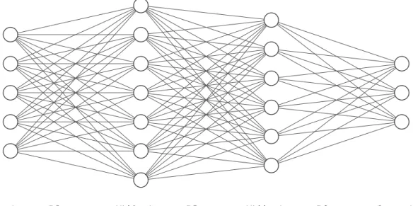
Input Layer ∈ ℝ Hidden Layer ∈ ℝ Hidden Layer ∈ ℝ Output Layer ∈ ℝ³

Figure 2.1.: Example of 3 layer fully-connected ANN. Each neuron (circle) is connected to all neurons of the successive layer.

One of the key attributes of these computational models is the composition of multiple interconnected processing layers. For each layer, the input data is transformed further, leading to more abstract representations and building a hierarchically structure of information processing. Probably one of the most prominent models in deep learning are Artificial Neural Networks (ANNs). Composed of multiple layers each containing various non-linear modules, often referred to as “neurons”, ANNs can represent any mathematical function [29]. An example of an ANN is shown in figure 2.1. The key technique to learn the respective input-output relation is called backpropagation. Thereby, the internal parameters, also known as weights, are adjusted to produce better representations and thus a more precise mapping.

(16)

2. Related work

In supervised learning, this is achieved by computing the error between the network output and the actual target value with a loss function. Computing the gradients of this function with respect to the weights, they can be adjusted to decrease the error.

Due to the increasing availability of computational power and the progress in effectively training neural networks, deep learning methods gained a lot of attention in the past decade, in particular since those methods have outperformed other techniques in applications like image [30] or speech recognition [31] by far. Like other natural signals, images can be decomposed hierarchically. This is why deep learning works so well in image processing. For instance, an image can be seen as a composition of edges creating motifs which make up parts and finally objects [29]. Using techniques as described in [32], this hierarchy can even be visualized as shown in figure 2.2.

Figure 2.2.: Visualizing hierarchy as described in [32]. Image obtained from [33] .

A famous example for the success of deep learning in image recognition is the winner of the ImageNet challenge [25] in 2012, AlexNet [30]. The task was to classify images into one of 1000 classes. For training, the ImageNet dataset contained 1.2 million labeled images at that point. Beating the second best candidate by over 10 percent in the top-5 test error rate, AlexNet marks a cornerstone in the development of deep learning and lead to increased popularity of a specific type of ANNs for image processing: the Convolutional Neural Network (CNN).

2.1.3. Convolutional neural networks

A CNN is composed of different type of layers, the most significant one being a convolutional layer. A so-called kernel, or filter, consisting of a set of weights and structured as a 3-dimensional tensor is shifted over different input regions by a predefined stride, applying matrix multiplication at each position (see figure 2.3). Stacking the results of several filters per layer forms a new output tensor.

The concept of sharing weights with different parts of the input reduces the number of trainable parameters and enables detection of local patterns independent of spatial location.

(17)

2. Related work

Figure 2.3.: Example of convolutional layer (adapted from [34]) .

Subsequently, the output tensor of the convolutional layer is transformed element-wise by a non-linearity, typically a Rectified Linear Unit (ReLU) [35].

Another commonly applied layer is the pooling layer which merges features that are semantically similar. Due to this setup of concatenating multiple stages of convolutional layer, non-linearity, and pooling layer, a CNN can learn to extract high-level features composed of low-level ones. This enables detection of features independent of their location, simultaneously being robust to some degree of variation.

A very successful architecture is the VGG net [36], named after the team that won the ImageNet challenge 2014. They used more layers than other network architectures at the time and small filter sizes of 3x3 for all of them.

However, very deep networks appeared to be hard to train due to the vanishing gradient problem. As weight gradients are computed by back-propagating the error through the network, repeated multiplication of preceding gradients may lead to infinitely small gradients. Consequently, the weights of early layers can not be adjusted and the network performance saturates.

It appeared that the performance of a trained network strongly depends on the initializa-tion of its weights. Thus, several studies examined normalizainitializa-tion approaches for weight initialization [37, 38, 39, 40]. Furthermore, normalizing layer inputs by integrating so-called Batch Normalization (BN) layers [41] into the architecture have become common practice. Another solution to prevent vanishing gradients even for very deep networks was proposed in 2016, describing deep residual learning for CNNs and presenting the architecture of ResNets [42]. The main characteristic in ResNets is an identity "shortcut connection". Here, the output of one layerxis directly forwarded to a later layer, skipping some layers in between, and then added to the output of the preceding layerF(x)(see figure 2.4).

(18)

2. Related work

+ Layeri Layeri+1

x _F₍_x₎ _F₍_x_{) +}_x

x

Figure 2.4.: Residual block in ResNets

The authors hypothesize that it is easier to optimize a residual mappingF(x) +xthan the original unreferenced mapping since the gradient in such a residual block is now enlarged by the derivation of the identity. Referring to empirical studies on ResNets [42], and the fact that this architecture won the 2015 ImageNet challenge [25], they indeed achieve better accuracies with deeper networks and avoid the problem of vanishing gradients.

Regarding pixel-wise classification of images (semantic segmentation) another architecture became widely popular. Fully Convolutional Networks (FCN) [43] use deconvolutions, or backward convolutions, for upsampling dense feature tensors back to the input image size predicting a class for each pixel. As for classification models, multiple stages of convolution, pooling and non-linearities produce abstract representations. Instead of a subsequent fully-connected (FC) network, these representations are processed by deconvolutional filters, which can be seen as convolutions with fractional input stride. Stacked together with activation functions, like ReLU, deconvolution allows learnable, non-linear upsampling. Furthermore, to combine global semantic information with local appearances, [43] also introduces skip connections from earlier layers with finer strides to the final output layer. Hence, higher-resolution features of the convolutional part are fused with the predictions of the last upsampling layer. Applying another convolution to the combined result, the network can learn to predict more precisely.

This idea is even extended in [44] describing an architecture originally applied for seg-mentation in medical images, called U-Net. Instead of only combining the last upsampling layer with the output from earlier convolutions, the U-Net architecture has a symmetric u-shaped structure of multiple skip connections between the downsampling and upsampling part of the FCN. The output from various layers during feature extraction (downsampling) is concatenated to the input of the corresponding layers in the upsampling process, sharing local information of the respective resolution and thus generating more precise segmentation masks.

2.1.4. Limits of supervised learning

The models described previously were all trained and evaluated in a supervised manner. There is a variety of labeled datasets commonly used for benchmarking new machine learning techniques or models, like ImageNet [25] for image classification, or PASCAL VOC [45] and COCO [46] for segmentation. Thus, for all images in the dataset, there exists a respective ground truth determining the target that should be predicted by the model. For image classification, the ground truth is the class corresponding to the depicted object, usually

(19)

2. Related work

represented by an integer. In segmentation tasks each pixel of the input image is classified separately. When comparing the model’s prediction with the corresponding ground truth using a specified loss function, the error can be evaluated and the gradients are computed using the backpropagation algorithm. Typically, stochastic gradient descent or some variant thereof is applied for updating the model. The model is shown a few examples of the dataset (a mini-batch), computes the output, errors, and gradients and then averages the gradients for a single update step.

However as mentioned before, a large amount of training samples is required to train a model that generalizes well to unseen data. Otherwise, the model may overfit, memorizing the ground truth of the training set instead of learning general distinctive features. To overcome this issue, it is important to cover different perspectives and possible appearances of a given class, such that the model can learn to create visual representations, required for determining the correct class. In practice, the acquisition of labeled datasets, i.e. data with corresponding ground truth, is time-consuming and sometimes even infeasible for millions of images. Therefore, application specific datasets are often magnitudes smaller than popular benchmarking datasets. Especially if the effort of annotation is high, as for segmentation, datasets are often limited to a few dozen to hundred samples. For instance, in [44] only 30 images with associated ground truth were used to train the U-Net. To deal with this problem, various techniques have been developed to prevent overfitting and train models that generalize well which are going to be discussed next.

2.1.5. Data augmentation and transfer learning

Data augmentation is a common technique to artificially enlarge an existing dataset. Either by randomly warping data samples during the training phase, e.g. applying affine trans-formations to the input, or by synthetically creating new instances and adding them to the training set which is called oversampling [47]. Figure 2.5 shows rotations/mirroring of an ASI as exemplary affine transformation.

Figure 2.5.: Example of image rotation/mirroring as data augmentation method for ASIs .

Another approach frequently applied for CNNs when data is limited, is transfer learning. A network is pretrained on a big dataset, like ImageNet, and the weights of the convolutional layers are used for initialization in the application task. Transfer learning can be applied to any vision task like classification, object detection or segmentation, provided that the downsampling architecture of the CNN is the same. Many image datasets share low- and

(20)

2. Related work

mid-level features which can be learned better on big datasets [48]. This is because of the hierarchical composition of image features leading to very general ones in early layers which become more and more specific in deeper layers (see figure 2.2). Even on dissimilar datasets, transferred weights usually show some benefit compared to random initialization such that it has become common practice to start training with pretrained weights. However, recent publications on transfer learning question the actual benefit of pretraining on datasets like ImageNet. In [49], it is shown that models with randomly initialized weights can reach competitive results on the COCO dataset [46] compared to the pretrained ImageNet counterparts. Regarding medical imaging, where image data is very different to ImageNet, it is concluded that only few pretrained filters contribute to useful feature extraction and the rest are too specialized from the original task [50]. Like in medical imaging, ASIs differ very much from datasets like ImageNet. For example, images often require higher resolutions in order to recognize the cloud type. Moreover, there is not necessarily a clear or unique target class within an image and there are considerably less classes overall. Therefore, recently another approach has gained a lot of attention in the computer vision community that allows to learn useful representations even if labeled data is not available.

Unsupervised and self-supervised learning

Unsupervised learning in general does not require a ground truth but it aims to discover underlying structures and patterns in the data. Apart from clustering or dimensionality reduction, learning representations with unlabeled data is a common task in unsupervised learning that has been studied intensively since the breakthrough of deep learning. The related approach of self-supervised learning [51] is a form of unsupervised learning. Within a so-called pretext task, the model learns visual representations in a supervised manner, but without any human-annotated labels which is why it is considered as unsupervised. This is achieved by extracting or generating the ground truth automatically from the image data. In the second part, the downstream task, the learned features are transferred to the model for the target application and the model is fine-tuned on a small dataset. The idea of self-supervision is to define a problem the model can only solve by learning important visual representations which are also useful for the actual target task. As the distinction between unsupervised and self-supervised methods is informal in the existing literature, in this work the more specific term self-supervised is used.

There are different approaches of visual representation learning that can be applied as pretext tasks. A survey on self-supervised learning [52] subdivides those methods into generation-based, context-based, free semantic label-based, and cross-modal based.

For generation-based methods, the auto-encoder is a well-known example. An auto-encoder consists of an encoding and a decoding part connected by a bottleneck layer. During the encoding, the input data is compressed into a latent-space representation and the decoder tries to reconstruct the input. A difference measure called reconstruction loss is then used for updating the model weights through backpropagation. The drawback of standard auto-encoding is that the model learns to reconstruct input noise as well. Vincent et al. presented a variant of stacked denoising auto-encoders for feature learning with deep networks. Later

(21)

2. Related work

CNNs were also used in terms of auto-encoding [54].

Another type of generative models that can be applied for unsupervised representation learning is the Generative Adversarial Network (GAN) [55]. The main characteristic of GANs is the competition of two networks trying to beat each other, like in a zero-sum game. While the generative part creates an output which should be similar to some given data distribution, the adversarial part aims to distinguish between the generated output and the true data. Although GANs are still relatively new, there are already a lot of examples where they were applied successfully. A famous version is the Deep Convolutional GAN (DCGAN) released in 2015 by Radford et al. who explicitly used GANs for representation learning. They trained one CNN to generate artificial images from a uniform distribution and another CNN to distinguish between artificially created and real images. The two networks improve each other as they try to get better in solving their respective task, the generative model by creating more realistic images, and the adversarial one by detecting finer details for discrimination. In another work, a GAN is used for predicting missing parts of an image [57], also known as inpainting. Here, the input is not drawn randomly from some distribution, but real images are corrupted by superimposing black boxes onto them. Hence, the model needs to learn to interpret the context by looking at surrounding areas of the missing parts in order to fill the boxes reasonably. Apart from creating artificial images or parts of it, GANs also have proven to be effective for superresolution [58]. Due to a perceptual loss, comprising pixel and adversarial loss, the model is forced to learn fine textures of a depicted object to produce realistic high-resolution images. The idea of including a perceptual loss for superresolution was also pursued in [59], introducing an extra loss from a trained and fixed convolutionalloss network[59]. It is computed by measuring differences in feature maps at different layers of the fixed network between target and predicted images. As a result, when textural features get lost during upscaling, the discrepancy in feature maps leads to a higher loss and eventually pushing the model to consider these features.

Context-based pretext tasks aim to learn context similarities or spatial/temporal structures. Spatial relation methods include predicting relative positions of two image patches [60] and solving jigsaw puzzles [61]. When video data is available, temporal relation can be learned by predicting the correct sequence from a randomized set of images obtained from a video [62]. A method which outperformed other state-of-the-art methods when applying learned representations directly in benchmarks for classification, detection or segmentation tasks was presented in [63]. It is based on learning image similarities by alternately clustering CNN features and training the CNN to solve a classification problem.As clustering technique, the k-means algorithm is applied which groups input vectors to a predefined number of clusters by calculating a distance measure between all samples. Next, the images are assigned pseudo-labels which correspond to the clusters that the CNN outputs were previously allocated to. Using these pseudo-labels, the CNN is trained to classify the images leading to updating its internal parameters and thus also to new features. Repeating this procedure the model can learn to classify images based on visual similarities.

(22)

2. Related work

2.2. Current techniques for ground-based cloud imaging

This section deals with the literature on classification and segmentation of clouds in ASI. Most of the times, previous studies have examined these tasks separately due to inherent complexity. Apart from few recent publications, cloud segmentation generally focused on solving a binary problem, distinguishing clear sky from cloud pixels. Starting with reviewing current classification methods, it is continued with those for binary segmentation and concluded with studies that address a more fine-grained segmentation.

2.2.1. Cloud classification

In general classification tasks, the goal is to assign a given input to a category that is part of a predefined set. As machine learning methods encompass suitable and effective tools for categorizing data into groups of specified characteristics, most approaches in cloud classification are learning-based. Typically, spectral, textural or structural features are extracted from images and fed into a classifier. Heinle et al. [64] proposed a k-nearest neighbor (kNN) classifier, assigning ASIs into one of seven classes that represent different sky conditions. The classes are defined by merging some of the official cloud types that have similar visual characteristics. Since multi-layer conditions occur frequently, images for training were selected manually to leave out ambiguous situations and show a clear dominant cloud type. With a focus on combining textural and structural features, Zhuo et al. [65] applies a Support Vector Machine (SVM) to classify feature vectors. The class definitions are adopted from [64], though one cloud type was omitted. Unlike in [64], only parts of an ASI, so-called sky patches, were classified to prevent ambiguous conditions. More recently, deep learning methods were tested, too. In [66], a CNN based model was presented, called DeepCloud. First, features are extracted by a CNN. Then they are processed to obtain more distinctive representations by applying discriminative local pattern mining and Fisher vector encoding [67]. Finally, classification is performed with a SVM. The dataset is the same as in [65], containing 1231 images, but with a more precise classification of nine cloud types as defined by the World Meteorological Organization (WMO) [68]. A regular CNN for cloud classification was presented in [69]. It is based on AlexNet [30] and achieved very good results on their own dataset. They also used official cloud generas for classification but added the class of contrails caused by aircrafts, resulting in 10 different classes.

It should be mentioned that comparisons are not expressive when different methods are not evaluated on the same dataset. Depending on the selection of images, there are easier or more difficult conditions for classifying clouds. For different observation sites, turbidity may vary substantially and complex multi-layer situations may occur more or less frequently. To my knowledge, the only current benchmark for classification was performed by Ye et al. in [66], comparing also the methods from [64] and [65].

(23)

2. Related work

2.2.2. Cloud segmentation

Automatic cloud segmentation from ground-based camera images has been studied intensively the last two decades. Sometimes also referred to as cloud detection, in this work the term segmentation is utilized for pixel-level classification, whereas detection indicates recognition independent of localization. Several threshold methods on color space information were developed to classify pixels into sky or cloud. Within the Red-Blue-Green (RGB) color space, the ratio [70, 71] or difference [64] between the red and blue color channel is a common measure. Due to increased scattering of blue wavelengths (Rayleigh scattering) in the atmosphere under clear sky conditions, the sky appears blue and the red-blue ratio (or difference) is smaller. For clouds however, Mie scattering is dominant leading to white or gray appearances. Other works propose to include the green channel as well [72] or transform the image into other color spaces, like HSI, and examine saturation [73, 74]. Furthermore, super-pixel segmentation has been investigated in [75]. Instead of classifying each pixel, an accumulation of pixels with similar textures and brightness are combined to super-pixels which are classified as a whole. Graph models outline another strategy. Each pixel [76] or super-pixel [77] is considered as a node connected to neighboring (super-)pixels by weighted edges. Taking some initial nodes that were classified with high confidence, the rest of the image is classified by evaluating a cost function for each node which depends on the edges providing information from surrounding nodes.

A problem with fixed thresholds is that they only work under certain conditions. For example, the RB ratio strongly depends on the relative position of individual pixels to the sun or to the horizon, in particular for atmospheric conditions with high amounts of aerosols. To address this challenge, Clear Sky Libraries (CSL) [16, 78, 79, 80, 81] were introduced. They contain historical RGB data acquired from clear sky conditions. By comparing a clear sky reference image with the image of interest, difficult conditions around the sun become easier to segment. For validating my deep learning approach, a CSL as described in [81] is also applied for binary segmentation on the same dataset in section 5.3.3. The CSL stores RGB values corresponding to Sun-Pixel-Angle (SPA), PZA, Air Mass (AM), and TL. SPA and PZA describe the relative position of pixels to the sun and the zenith (see figure 2.6). AM is a measure for the relative path length of solar rays through the atmosphere and TL specifies the fraction of incoming solar irradiance compared to ideal, clear and dry atmospheres.

The CSL consist of multiple layers, each corresponding to a specific AM and TL. Within a layer, RGB values from clear sky conditions are stored with respect to SPA and PZA. To distinguish between cloud- and sky-pixels, a clear sky image is generated from the layer that reflects current TL and AM best. Color features from the target image, like RB ratio, are then compared with the ones from the reference image. Detection is determined by multiple thresholds depending on SPA, PZA and the current weather situation which is estimated by considering recent fluctuations in irradiance measurements. An illustration of the workflow of the CSL is depicted in figure 2.7.

(24)

2. Related work

Figure 2.6.: Illustration of PZA and SPA for ASIs.

(25)

2. Related work

Over the past years, also some machine learning-based methods for cloud segmentation were presented. A systematic study on color spaces, applying Principal Component Anal-ysis (PCA) and fuzzy clustering to identify the most relevant color components for cloud segmentation is applied in [82]. In another work [83], Dev et al. review machine learning techniques for ground-based image analysis. Particularly a set of feature extraction methods like dimensionality reduction, sparse representation and classic image feature extractors are discussed within the context of segmentation, classification and denoising. One of the first applications of neural networks for ground-based cloud images was published in [84]. In this study, a shallow FC ANN is compared to a SVM, both showing significant performance boost over a threshold-based method used for validation. Although this dataset contains images from different conditions of cloudiness, the models are only trained and tested on extracted pixels from 15 images in total. Later, multiple supervised learning methods, like random-forest, SVM, and Bayesian classifiers as well as combinations of multiple classifiers were examined in [85]. For training, feature vectors are constructed by concatenating values of different color spaces as well as the RB ratio for each pixel. Furthermore, color components of local patches are added to create multiple feature vectors for each pixel in order to integrate information from neighboring pixels. Here, the classifiers were trained on 250 images with the best model achieving an average accuracy of about 90% for 10-fold cross validation.

As deep learning achieved outstanding performance improvements in other computer vision tasks, there has been increased interest in CNNs for cloud segmentation from ASI. Most recently, three academic papers were published tackling the issue of cloud segmentation with CNNs [86, 87, 88]. All of them follow a purely supervised approach with an encoder-decoder architecture based on the original FCN [43]. The model presented in [87], called SegCloud, was trained and tested on 340 and 60 annotated all-sky images respectively and outperformed a R/B threshold based approach by a large margin. Song et al.[88] conducted an extensive study of popular deep learning segmentation architectures by applying them on a dataset of sky patches [89].

Since there exists a variety of different approaches for cloud segmentation, benchmarks are an important tool to compare them with each other and to identify strengths and weaknesses. This is in particular because most approaches use individual datasets which have different characteristics. While some datasets consist of sky patches, intentionally omitting areas of the sun to prevent overexposure, others comprise ASIs from different devices. A comparison of various methods was conducted on two datasets of sky patches in [89], including the techniques described in [70, 73, 71] and their own probabilistic model [90] which achieved the best results.

Another very recent benchmark evaluates the performance of multiple methods on ASIs [91]. The utilized dataset focuses especially on covering a high diversity of atmospheric conditions and includes 829 manually segmented ASIs in total. Multiple current state-of-the-art techniques are evaluated on this dataset (multicolor criterion [72], CSL [80], Hybrid Thresholding Algorithm (HYTA) [71], region-growing [92] and FCN [43]). Although the FCN achieved the best results, it has to be considered separately, as a cropped rectangle from the ASI is segmented.

(26)

2. Related work

All aforementioned methods perform only binary segmentation, classifying a pixel either as cloud or no-cloud. However, regarding precise prediction of solar irradiance, a more fine-grained differentiation between clouds is beneficial [93]. One of the first attempts was performed by Dev et al. distinguishing between thin and thick clouds in a probabilistic framework [90]. Modeling the classes (thin/thick cloud, sky) as multivariate Gaussian distribution, the joint probability distribution of classes and image regions is learned by training with a small set of 32 labeled images. Afterwards, Dev et al. proposed a U-Net, trained on the same dataset, and compared the results to their previous approach [86]. Despite the limited amount of data, the CNN performs better, in particular for thin clouds.

Recently, another method has been published [94], addressing the problem of pixel-wise classification of cloud genera as defined by the WMO in [68]. The authors propose a supervised learning-based segmentation divided into several processing steps. First, super-pixel segmentation is applied to subdivide the image into small similar regions. For each super-pixel, feature vectors are created, based on color, internal and regional texture, as well as global relationships. Due to the nature of clouds, those feature vectors may still be very similar, which is why they apply a feature transformation based on subspace alignment and metric learning to receive more discriminative features. Classification is then performed on the transformed vectors using a SVM. For validation, they compared their approach with a pretrained FCN, beating it by almost 7% points on average. They argue that their dataset of roughly 600 images is too small for a deep learning approach to learn useful features but emphasize that there is potential when more data is available for training deep networks.

(27)

3. Datasets of All-Sky Images

Selecting suitable data for training deep learning models is essential to achieve good gener-alization. This chapter briefly presents the framework conditions for ground-based cloud observation. The main part deals with the new dataset that was created for supervised classification and segmentation. The process of annotating ASI datasets and a comparison with other datasets from the literature is presented. In addition, the selection of ASIs for self-supervised representation learning is described. Apart from a high variety of atmospheric conditions, it is also important to have a balanced distribution.

3.1. Utilized hardware and observation site

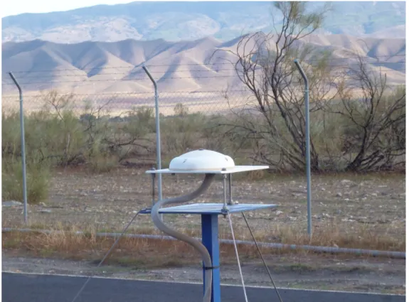
All image data for the new dataset was collected from the Plataforma Solar de Almeria (PSA) in the desert of Tabernas (Spain) which is operated by CIEMAT1. The utilized All-Sky Imager is based on an off-the-shelf surveillance camera from the manufacturer Mobotix (model Q25). Figure 3.1 shows one of the installed devices on the PSA. Its maximal resolution is limited to 6 MP. However, for compatibility with the previous Q24 model, the images are cropped and resized to a resolution of 2048 x 1536 pixels (3 MP). The exposure time is set to 160µsas previous studies showed that current state-of-the-art methods, like the CSL, work best with a fixed exposure time [81]. A Q25 model from Mobotix costs around 800 EUR in 2020. Images are obtained from a single device which is part of a meteorological station at the CSP test stand "Kontas". An image is taken every 30s from sunrise to sunset, leading to approximately 1800 images per day in summer.

3.2. Creation of an annotated All-Sky Image dataset

In the following section, the selection and annotation process for the new dataset is presented. It starts with a discussion about how the ASIs are classified, providing definitions of the utilized labels. Next, the manual segmentation and labeling process is briefly introduced. Finally, the selection of images and the variety of atmospheric conditions are discussed.

1_{Centro de Investigaciones Energéticas, Medioambientales y Tecnológicas: A spanish research institute with}

(28)

3. Datasets of All-Sky Images

Figure 3.1.: Picture of a Mobotix camera for taking ASIs

3.2.1. Selection of images and ground truth creation

For the creation of this dataset, images were annotated on pixel- and image-level to train models for classification and segmentation. A particular feature of the classification approach is to train a model to predict multiple labels for a given sample image instead of a single class. The terminological difference between label and class is that a sample can be assigned either a unique class or multiple labels that are not necessarily mutually exclusive. In preceding studies [89, 91], a model’s performance was analyzed by examining the results on different types of cloudiness and atmospheric conditions, for instance, by comparing the segmentation accuracy for clear sky and overcast conditions. In this work, a model shall also be capable of predicting such cloudiness characteristics. As mentioned in section 1.2, local pixel-level information is especially important for solar irradiance estimations in circumsolar regions. However, global information regarding overall cloudiness is also beneficial for nowcasting systems. For example, determining whether the sun is completely free from clouds is required to run qualification tests of solar power plants. Moreover, if a model reliably detects the degree of cloudiness, this information can be used to validate results from segmentation that should correspond to the prediction of the cloudiness label.

To distinguish between cloud types, a ternary categorization was chosen. As depicted in figure 3.2, the ten main cloud generas [68] can be split into three layers. Depending on where a cloud genus typically emerges, it is classified either as low-, middle-, or high-level cloud.

(29)

Figure 3.2.: Illustration of main cloud generas defined by the WMO [95]. The ten cloud types: Cumulus (Cu), Stratus (St), Stratocumulus (Sc), Cumulonimbus (Cb),Altocumulus (Ac), Altostratus (As), Nimbostratus (Ns), Cirrus (Ci), Cirrocumulus(CC), Cirro-stratus (Cs) can be grouped by their base height.

Height, unlike altitude, indicates the vertical distance from the point of observation to the cloud. However, there is no clear border between those levels. Firstly, clouds can extend over multiple layers, as thunderclouds (Cumulonimbus) typically do. Secondly, cloud layer heights depend on current atmospheric conditions, like humidity, temperature or pressure and can vary from one day to the other. Lastly, the observation site’s latitude has a significant impact on what height a cloud type occurs. Nevertheless, a subdivision of the 10 ten generas into three groups corresponding to the base height is appropriate for the approach pursued in this work. Primarily, optical characteristics of clouds within one layer are similar [93]. For example, clouds within the lowest layer are rather dense water clouds that often appear gray from beneath as a lot of solar irradiance is absorbed. On the other hand, high-layer clouds consist of ice particles only. They often appear hazy, are less densely distributed and have higher transmittance. In the mid-layer, clouds can contain water and ice particles. Hence, the transmittance is usually in between low- and high-level clouds. Another reason for this choice of categorization is the occurrence of different wind directions in the atmosphere. When detecting clouds in multiple layers, they may have distinctive directions of motion, even opposing ones. To track and predict future spatial expansion of all clouds, it is therefore

(30)

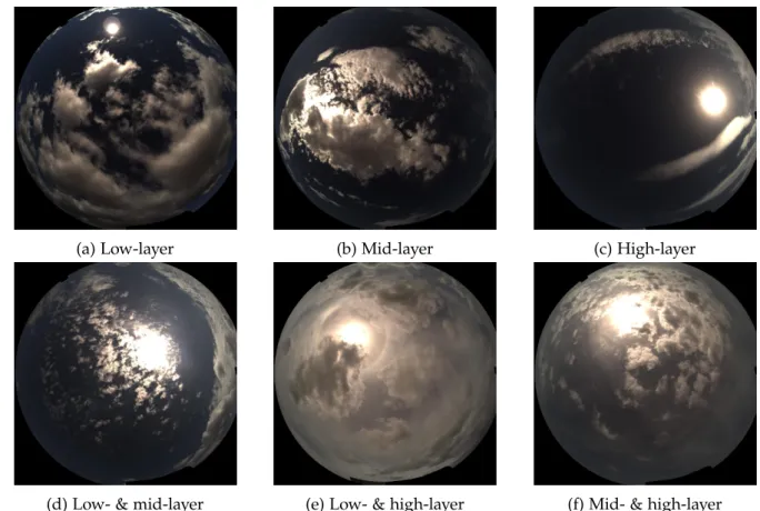
necessary to distinguish between clouds of different heights. Figure 3.3 shows exemplary clouds from single and multiple layers. In table 3.1, a summary of the presented categorization of clouds is shown with a brief description of each cloud type.

(a) Low-layer (b) Mid-layer (c) High-layer

(d) Low- & mid-layer (e) Low- & high-layer (f) Mid- & high-layer Figure 3.3.: Examples of single and multi-layer ASI

Besides pixel-wise annotation of images indicating the cloud type, the image itself is labeled with all layers that are depicted. Hence, it can be examined if the classification model is able to detect the layers correctly regardless of their precise location. Furthermore, five other labels that can be assigned to each ASI were defined. The labelsClear Sky,Overcast,Cloudy-SV(sun visible),Cloudy-SC(sun covered) describe the form of cloudiness and are mutually exclusive. They are based on cloud coverage and the visibility of the sun. The last label is calledSun Freeand determines if the sun disk is completely free from clouds. A summary of all labels can be found in table 3.2.

The dataset presented here is based on the data from the benchmark of binary segmentation methods in [91]. Overall, 669 images from the Kontas Q25 camera and corresponding binary masks were taken and revised. The masks were originally created with a Matlab graphical user interface (GUI) implemented using the Matlab GUIDE framework. To integrate functionality of classifying pixels into different cloud types and to ensure compatibility with future Matlab versions, a new GUI was implemented with Matlab’s App Designer.

(31)

Table 3.1.: Categorization of cloud types used for semantic segmentation adapted from [95] and [96]. Height level is valid for mid-latitudes regions, like Southern Spain. Class Height Level Cloud Genera Characteristics

High-Layer > 6 km

Cirrus Detached, white, fibrous filaments, narrow bands

Cirrocumulus Thin, white, very small elements without shading

Cirrostratus Transparent, whitish cloud veil, fi-brous or smooth

Mid-Layer 1.8 – 8 km

Altocumulus White and/or gray, small elements with shading

Altostratus Grayish/Blueish layer, fibrous or uniform

Low-Layer 0 - 2.4 km

Cumulus Sharp outlines, detached, develop-ing vertically, dark bases

Stratus Fairly uniform gray base, no clear outlines

Stratocumulus Gray and/or whitish, visible out-lines

Cumulonimbus Heavy, dense, large vertical extent (over all layers)

Nimbostratus Gray (often dark) layer, can extend to high-layer

Table 3.2.: List of image-level labels defined in the new dataset. Label Name Definition

Clear Sky Less than 2% of the sky is covered with clouds and the sun disk is free.

Overcast More than 95% of the sky is covered with clouds.

Cloudy-SV The sky is partially clouded and the sun is visi-ble but not necessarily free.

Cloudy-SC The sky is partially clouded and the sun is cov-ered such that the disk cannot be recognized. Sun Free No cloud is in front of the sun disk.

Low-Layer Low-layer clouds (e.g. Cumulus) are visible. Mid-Layer Mid-layer clouds (e.g. Altostratus) are visible. High-Layer High-layer clouds (e.g. Cirrus) are visible.

(32)

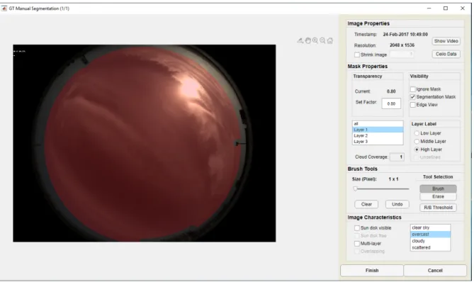
The process of adding new images and creating corresponding ground truth is described briefly in the following. First, the user selects the dataset of interest which is organized via a tabular Matlab file. Next, the parameters to search for images are chosen. In addition to specifying the time frame of interest, the user can also filter for a range of TL and Solar-Zenith-Angle (SZA). If there are images matching the chosen parameters, a random sample is displayed that can be added to the dataset or discarded. Afterwards, the image is pre-segmented using a CSL to decrease the effort of manual editing. Moreover, a camera specific mask is applied which defines the region of interest within the sky image. Hence, static objects that are in the field of view of the camera can be excluded. The same way areas very close to the horizon can be ignored which are affected most by distortion effects and vignetting and thus are not clearly identifiable. Finally, the image is segmented manually using various editing tools and classified by selecting the correct checkboxes.

Figure 3.4.: Matlab GUI that was implemented to manually segment ASIs

A crucial difference to the original dataset is the distinction between aerosols and high-layer clouds. In most previous works, the focus was on detecting clouds that are clearly distinctive from aerosols. Hence, difficult cases showing thin ice clouds were either left out completely or these pixels were declared as clear sky. Since they still have a notable influence on solar irradiance, the dataset was extended to include these situations, too. However, aerosols and thin cloud sheets are still distinguished. As can be seen in figure 3.5, turbid atmospheric conditions affect the size of the sun disk. To check whether this mainly comes from stratus-like ice clouds, analyzing the video data proved to be helpful. If clear motion patterns can be recognized, thin high-layer clouds can be assumed. When the atmosphere is clear and the

(33)

sun disk is small, high-layer clouds may still be difficult to detect (see figure 3.5d). Cirrus clouds have more texture but are often only visible in circumsolar regions. They do not show clear contours and pixels with larger distance to the sun slowly merge with the sky.

(a) Clear sky, low TL (b) Clear sky, high TL (c) High-layer, high TL (d) High-layer, low TL Figure 3.5.: Comparison of aerosols and high-layer clouds

In summary, existing segmentation masks were updated to include layer specification and to consider difficult high-layer pixels. Furthermore, the dataset was extended by roughly 100 images. Most of them were images with multi-layer and high-layer conditions to achieve a more balanced distribution.

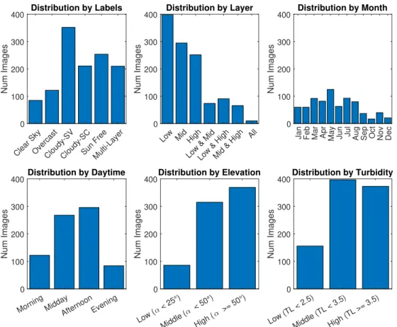
To ensure that a high variety of atmospheric conditions is represented, the dataset was examined by filtering via various parameters. The following plots in figure 3.6 show the distribution corresponding to the label definitions, sun elevation, daytime, month, and TL. Generally, clear sky conditions are easy to detect and thus less images were selected. Nonetheless, different TLs are required for the model to learn to distinguish between aerosols and high-layer clouds. A large variation in sun positions was obtained by including images from an entire year and different daytimes. However, very low sun elevations (< 8°) were discarded. On the one hand, those images are often too dark to correctly detect clouds, as the exposure time is fixed. On the other hand, large AMs due to low sun elevation angles lead to energetically speaking less interesting conditions for solar power applications. The distribution of layers is not completely balanced, but even high-layer clouds are represented approximately every third image. Multi-layer conditions make up a quarter of the dataset. Each combination is represented similarly, apart from the scarce case with all layers visible in one image.

(34)

Distribution by Labels

Clear SkyOvercast_Cloudy-SV_Cloudy-SCSun Free Multi-Layer 0 100 200 300 400 Num Images Distribution by Layer

Low Mid High

Low & Mid_{Low & High}Mid & High All 0 100 200 300 400 Num Images Distribution by Month

Jan Feb Mar Apr _May Jun Jul Aug Sep Oct Nov Dec

0 100 200 300 400 Num Images Distribution by Daytime

Morning Midday_{AfternoonEvening}

0 100 200 300 400 Num Images Distribution by Elevation Low ( < 25°) Middle ( < 50°) High ( >= 50°) 0 100 200 300 400 Num Images Distribution by Turbidity Low (TL < 2.5) Middle (TL < 3.5)High (TL >= 3.5) 0 100 200 300 400 Num Images

Figure 3.6.: Distribution of data according to different parameters.

3.3. Comparison to other cloud datasets

There are multiple reasons for creating a new dataset to develop deep learning models for cloud classification and segmentation. First, most datasets mentioned before do not meet the requirements for semantic cloud segmentation under multi-layer conditions, since they only include binary masks. Moreover, not all of them provide all-sky images but only sky patches. Lastly, only few datasets are publicly available. In this section, the most relevant datasets from the literature are briefly discussed and contrasted with the new dataset described in section 3.2.

In [64], approximately 1500 manually selected all-sky images were used. They were taken from a research ship on its way from Germany to Africa and thus covering different climate zones, atmospheric conditions and SZA. The ground truth includes a binary segmentation mask as well as the dominating cloud type within the image. Seven cloud types are distin-guished which are based on the main generas, but merging some visually similar generas like Altostratus and Stratus. To avoid ambiguous cases, only single-layer images were selected to ensure unique classification, on average 200 per class. As the goal is to develop models that

(35)

work under all possible conditions, it is crucial to integrate complex multi-layer conditions. Hence, in this work a coarser classification was chosen, but trained and validated on a more realistic dataset.

Publicly available datasets are HYTA [71] and Singapore Whole-sky Imaging Categories/Seg-mentation (SWIMCAT [97], SWIMSEG [89]). All of which consist of sky patches that were extracted from ASIs. HYTA contains 32 binary segmented images of four categories: cu-muliform, cirriform, stratiform and clear sky. Later a ternary version was developed in [90] where cloud pixels are categorized in terms of optical thickness: thin-/thick clouds and sky. SWIMCAT/SWIMSEG were presented in [97] to address the lack of public datasets. The former includes 784 patches in total, each annotated on image-level with one of five cloud types, namely: clear sky, patterend clouds, thick dark clouds, thick white clouds, and veil clouds. The latter contains 1013 patches with binary segmentation masks, in consideration of varying atmospheric conditions.

Another dataset of sky patches is used in [65] and adapted in [66]. It provides image-level annotations of 1231 images, originally grouped into 6 classes as proposed in [64], and later updated to match the official main cloud types. Probably the largest labeled dataset of cloud images is Cirrus Cumulus Stratus Nimbus (CCSN) [69] used for training CloudNet. It contains 2543 images of natural images of ten cloud types taken at various locations. Occasionally, some images include surrounding landscapes which is different to the other datasets that only include sky patches. Since all these datasets only capture small parts of the hemisphere, they cannot provide as much information as ASIs and are not suitable for nowcasting systems.

Recently, a very detailed dataset was presented (but not made publicly available) in [94]. It is the first approach of classifying nine main cloud types pixel-wise in ASIs. A team of experts manually created 600 ground truth masks of images obtained from two different locations in China with different air qualities.

The benchmark for binary segmentation from ASIs [91] contains 829 images and corre-sponding binary masks. The images were taken from two cameras and selected manually to cover a high variety of atmospheric conditions. As previously mentioned, parts of the dataset presented here were adapted from [91]. Furthermore, new images of primarily multi- and high-layer conditions were added, resulting in 770 images with respective ground truth. An overview of the described datasets can be found in table 3.3.