Abstract: In this paper, we proposed a fusion feature extraction method for content based image retrieval. The feature is extracted by focusing on the texture and shape features of the visual image by using the Local Binary Pattern (LBP – texture feature) and Edge Histogram Descriptor (EHD – shape feature). The SVD is used for decreasing the number of the feature vector of images. The Kd-tree is used for reducing the retrieval time. The input to this system is a query image and Database (the reference images) and the output is the top n most similar images for the query image. The proposed system is evaluated by using (precision and recall) to measure the retrieval effectiveness. The values of the recall are between [43% –93%] and the average recall is 64.3%. The values of precision are between [30%-100%] and the average is 72.86% for the entire system and for both databases.
Keywords: CBIR, Global features, LBP, EHD, SVD, Kd-tree, Image retrieval.
I. INTRODUCTION
T
he feature extraction phase plays a significant role in image retrieval as the performance of the system much based on the ability of these extracted visual features in characterizing the image content. The features extracted are the numerical values data obtained from images that are hard for a human being to understand. The size of the features derived from an image is much reduced than the original image. Dimensionality reduction decreases the overheads of processing the image bunch. There are two kinds of features obtained from the image: local and global features. Global features are defined for characterizing the image as a whole, which is used for image retrieval, object detection, and classification. While local features are limited to describing the image patches which are used for object recognition and identification. Combining global and local features increases the precision of recognition with the negative effect of cost computing.Numerous features can be extracted from the image; among which, the color, shape and texture features are well- studied and extensively used for CBIR applications. Also, local features such as Scale Invariant Feature Transform (SIFT) [1] and Speeded Up Robust Features (SURF) [2] have also gained attention because of their invariance property and performance in object retrieval.
Revised Manuscript Received on September 03, 2019
* Correspondence Author
Abdulkadhem Abdulkareem Abdulkadhem*, Department of Software, College of Information Technology, University of Babylon, Hillah, Iraq.
Email : [email protected]
Tawfiq A. Al-Assadi, College of Information Technology, University of Babylon, Hillah, Iraq.
Email: [email protected]
Color is a low-level visual feature which it the most efficient, comfortable and commonly used in CBIR. Human visual perception can easily discriminate different colors compared to other features. It is also a robust feature, as it does not based on the situation of the image, such as the direction, size, and angle. According to various application requirements, color features can be defined over different color spaces such as RGB, HSV, YCrCb, etc. [3]. The commonly used color descriptors include color histogram, color coherence vector [3], color moments [4], color- correlogram [5], color auto correlogram [6] and color co-occurrence matrix [71].
Another significant visual feature is texture. Texture can be interpreted as continuous patterns of local variation for intensity pixel. In contrast to color, a texture occurs in an image region (collection of pixels), while color occurs on an image point (pixel). Image features like contrast, coarseness, directionality, regularity, entropy, etc. can be extracted with various texture descriptors. There are many techniques applied for computing the texture features such as fractals, wavelets, co-occurrence matrix, Gray Level Co-occurrence Matrix (GLCM), Local Binary Patterns (LBP), Tamura features, etc. [3, 8 and 9].
In other methods like spectral texture approaches, images are transmuted into the frequency domain by employ particular spatial filter methods. Texture features are taken from the transformed spectra using statistics. Due to the large neighborhood support of the filters, spectral techniques are powerful to noise. Common spectral methods include Fourier transform, discrete cosine transform (DCT), wavelet transform and Gabor filters [3, 10, 11 and 12].
Shape features are often applied effectively for particular uses involving man-made objects. However, as these features are susceptible to image transformations like translation, scaling, and rotation, they are not as popular as color and texture features in retrieval applications and are often used in conjunction with other image features. The edge histogram descriptor (EHD) is one of the commonly used approaches for shape detection [13].
Our content-based image retrieval method depends on global features of images. The proposed system focuses on the texture and shape features by using the Local Binary Pattern(LBP) and Edge Histogram Descriptor (EHD) features, respectively. Each image in database represented by (256,1024,..,etc) bins for LBP and 150 bins for EHD. The Singular value decomposition (SVD) is used to compress the length of image features to only six features for each image while Kd-tree is used to extract
the top N comparable images for a query image.
Proposed a Content-Based Image Retrieval
System Based on the Shape and Texture Features
II. THEPROPOSEDSYSTEM
[image:2.595.49.288.110.571.2]The proposed system of this paper consists of many stages, and each stage has several steps. The block diagram of the proposed system is illustrated in Fig 1.
Fig 1. The block diagram of the proposed system. A. The input query image and preprocessing
In this stage, the first step is converting the query image and database images from 24-bit color RGB (Red, Green, Blue) to grey-scale form. The next step of this stage is preprocessing and filtering process involving noise removal, smoothing, and enhancement of the frames of video by using low pass filtering, high pass filtering or median filtering.
B. Feature Extraction.
In this stage, we suggested a fusion method for feature extraction by focusing the texture and shape features of the visual image by using the Local Binary Pattern (LBP – texture feature) and Edge Histogram Descriptor (EHD – shape feature). The input to this stage is the query image and the database images and the output is the feature matrix. 1- Applying the LBP.
In this step, the feature vector will be extracted by using the Local Binary Pattern (LBP) for each reference image in the
database and the query image. Each image has a huge number of pixels, thus we need a method to extract a feature vector that represents the image. Suppose we have an image with size(300*300) pixel, which means that we have 90,000 pixels representing the image. The goal of using the LBP is to decrease the features pixel from 90,000 to (256, 1024 or 2304) feature vector. The LBP for an image is extracted according to the following steps of the algorithm (1) illustrated bellow.
Algorithm (1): Local Binary Pattern (LBP) algorithm
Input: A grayscale image with size (m,n). Output: A grayscale image with size (m,n). Begin
1- Scan the image of size (m*n) by using a sliding window with size 3*3.
2- For each window represent the neighbour correlation of center pixel to binary by the threshold. The code is 0 if the neighbour pixel less than or equal to the center pixel while the code is 1 if the neighbour pixel largest than the center pixel.
3- Read the binary code of 8- neighbour of the window in a clockwise or counterclockwise direction and collect 8-binary code
4- The 8- digit binary code is converted to decimal number.
5- Put the decimal number on the center of the window.
end
[image:2.595.307.558.482.642.2]Now, the final result of this step is an image with size (m*n) with different values compared with the original image that represents the Local Binary Pattern of image. Fig 2. represents the illustration of applying a Local Binary Pattern (LBP) on an image.
Fig 2. An example of Local Binary Pattern (LBP) on an image.
2. Dividing the LBP Image to Number of Region
Fig3. Dividing the LBP image to regions.
3. Extracting the Histogram for each Region.
A histogram is a perfect representation of the spreading of pixel color values in image processing. It is an evaluation of the probability distribution of each gray-level value in the image. After determining the number of regions for LBP-image, now the system will compute the histogram for each region which values of each histogram bin between (0-255) that represent the range of gray-scale values.
4. Concatenating all Histograms as a Vector
[image:3.595.304.549.125.229.2]In this step, the system will merge the histograms of the image as a single histogram. The first histogram region takes values between 0 and 255. The second one takes values from 256 to 511. The third one takes values from 512 to 767 and so on. Each value represents the number of its occurrences in a particular region in LBP-image. Fig 4. represents the concatenated collection of histograms to one which is considered a feature vector for a particular image.
Fig 4. Concatenation histograms.
[image:3.595.309.542.326.492.2]5. Applying the Edge Histogram Descriptor (EHD) The EHD reflects the distribution of 5 kinds of edges in each local region termed a sub-image. The sub-image is described by splitting the image space into 4 non-overlapping blocks, as shown in Fig 5 So, whatever the size of the actual image, the image division produces 16 equal sub-images.
Fig 5. Sub-image and image block definition.
We then produce a distribution edge histogram for every sub-image to describe the sub-images. The sub-image edges are classified into five kinds of edges: horizontal, vertical, 45-degree diagonal, 135-degree diagonal and non-directional, as described in Fig 6. which explains the shape of edges and their filters.
Fig 6. Five types of edges and filters.
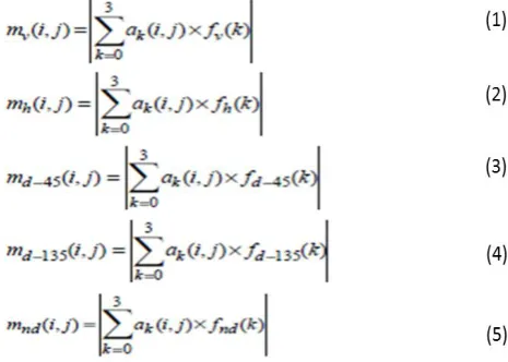
The five kinds of edges can be extracted by filtering image depend on the convolution matrix. Convolution is the treatment of a matrix by another one which is called “kernel”. Equations from (1) to (5) explains the five types of filtering processes.
The five types of edges can be extracted by filtering image based on a convolution matrix. Convolution is the treatment of a matrix by another one which is called “kernel”.
[image:3.595.54.287.422.544.2]Thus, for each sub-image, the histogram describes the relative frequency of occurrence in the corresponding sub-image of the 5 edge types. As a direct result, as shown in fig 7., there are 5 bins for each local histogram. Each bin refers to one of five kinds of edge. Since, the image contains 16 sub-images, a total of 5 x 16=80 histogram bins are needed, as illustrated in Fig 8.. Note that with regard to location and type of edge, each bin of 80-bins histogram has its own semantics.
[image:3.595.53.288.637.752.2]Fig 8. A 1-D array of EHD 80 bins.
[image:4.595.49.287.56.172.2]The complete EHD semantics with 80 histogram bins are summarized in Table- I. When there is an edge, the predominant edge kind is also determined among the 5 edge classifications. Then, the corresponding edge bin (the histogram value) is increased by one
Table- I: Semantics of local edge bins.
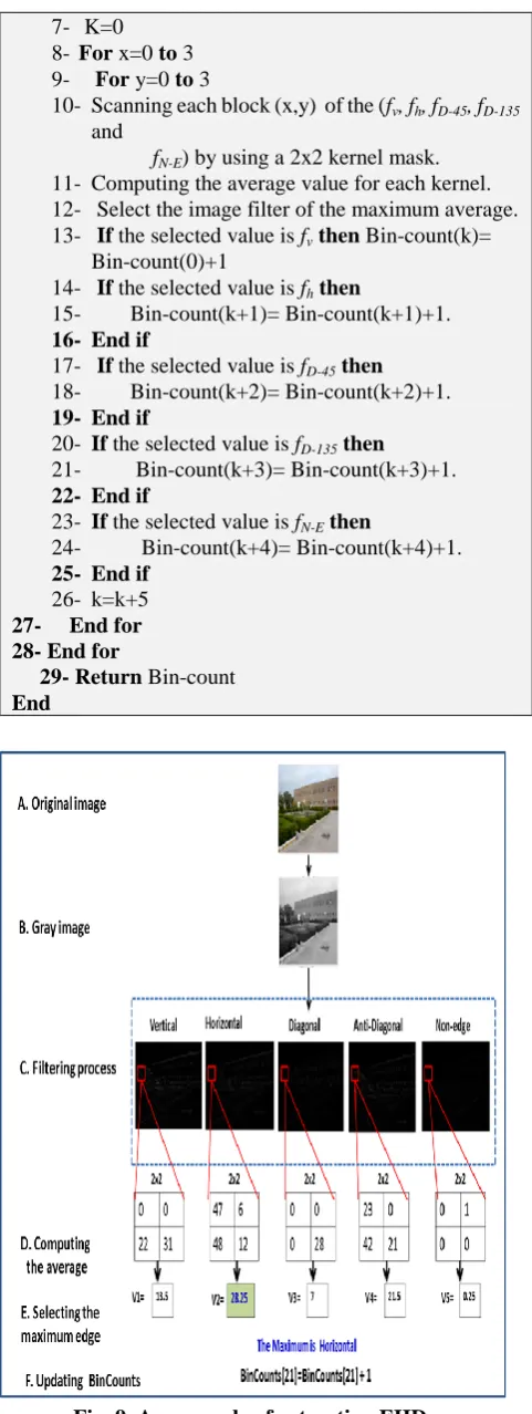
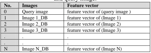
Algorithm (2) illustrates the pseudo-code of the Edge Histogram Descriptor (EHD) algorithm for an image (gray) while Fig. 9. illustrates the example of extracting the edge histogram descriptor for sub-block image of size (2x2) on sub-image (1,0) of the Fig. 4..
Algorithm (2): Edge Histogram Descriptor (EHD) algorithm
Input: A grayscale image with size (m,n). Output: A Bin-Count[80] vector . Begin
1- Computing the vertical filter for the image using equation (3.3) to produce fv. /* fv represents the vertical filter for input image*/.
2- Computing the horizontal filter for the image using equation (3.4) to produce fh. /* fh represents the horizontal filter for input image*/.
3- Computing the diagonal -45 degree filter for the image using equation(3.5) to produce fD-45. /* fD-45 represents the vertical filter for input image*/.
4- Computing the diagonal – 135 degree filter for the image using equation (3.6) to produce fD-135. /* fD-145 represents the vertical filter for input image*/.
5- Computing the Non-edge filtering image using equation (3.7) to produce fN-E. /* fN-E represents the non-edge filter for input image*/.
6- Dividing each of the (fv, fh, fD-45, fD-135 and fN-E) into non-overlapping 4x4 blocks.
7- K=0 8- For x=0 to 3 9- For y=0 to 3
10- Scanning each block (x,y) of the (fv, fh, fD-45, fD-135 and
fN-E) by using a 2x2 kernel mask. 11- Computing the average value for each kernel. 12- Select the image filter of the maximum average. 13- If the selected value is fvthen Bin-count(k)=
Bin-count(0)+1
14- If the selected value is fhthen
15- Bin-count(k+1)= Bin-count(k+1)+1. 16- End if
17- If the selected value is fD-45then 18- Bin-count(k+2)= Bin-count(k+2)+1. 19- End if
20- If the selected value is fD-135then 21- Bin-count(k+3)= Bin-count(k+3)+1. 22- End if
23- If the selected value is fN-Ethen
24- Bin-count(k+4)= Bin-count(k+4)+1. 25- End if
26- k=k+5 27- End for 28- End for
29- Return Bin-count End
Fig. 9. An example of extracting EHD.
6. Global, Simi-Global and Local Features of EHD. The only normative semantics for the EHD are the 80 bins of a local edge histogram (i.e., BinCounts [i], i = 0, ... 79) as explained in Table- I. However, the histograms of only the local edge may not be enough
[image:4.595.53.283.261.441.2]words, for the complete image space and specific vertical and horizontal semi-globe edge, in addition to local ones, we may need the information on the edge distribution. Fortunately, we can produce the global and particular semi-global edge histogram from BinCounts [i], i = 0, ... 79 directly at the matching step. The global edge histogram is the distribution of the edge for the complete image space. There are 5 kinds of edges, thus, there are 5 bins in the global edge histogram and each bin value is acquired by accumulating and normalizing the dequantized bin values of the corresponding edge type of BinCounts []. Similarly, we can cluster some subsets of BinCounts [] for the semi-global edge histograms as explained in Fig. 10. The 13 different parts (that are, 13 distinct subsets of the image blocks) are defined, and edge distributions for each section can be generated from 80 local histogram bins in five different edge types. Therefore, we have a total of 150 bins (5 bins (global) + 65 bins (13 x 5 semi-global) + 80 bins (local)) for similarity comparison.
Fig. 10. Sub-image segments for semi-global histograms.
7. Constructing the Feature Matrix
[image:5.595.310.541.300.429.2]In this step, we build the feature matrix of the database and one query image. Each row of the feature matrix represents the feature vector of one image (the concatenated histogram from the above step). The first row represents the feature vector of one query image, while other rows represent the feature vector of the reference images that are stored in the database. The length of each feature vector is (256,1024,2304, 4096,…), depending on the number of regions grid of dividing LBP-images plus (150 bins) of EHD. The 256 are used when the whole image as one region. The 1024 (256*4) are used when the image is split to four regions. The 2304 (9*256) are used when the image is split to nine regions. The 4096 (16*256)are used when the image is split to sixteen regions and so on. The size of the feature matrix is (N+1 * length of concatenated histograms). When N represents the number of reference images are saved in the database. The shape of the final result for this step explained in Table- II.
Table- II: The feature matrix representation of the database and query image.
No. Images Feature vector
0 Query image feature vector of (query image ) 1 Image 1_DB feature vector of (Image 1) 2 Image 2_DB feature vector of (Image 2) 3 Image 3_DB feature vector of (Image 3)
. . .
. . .
N Image N_DB feature vector of (Image N)
C. Applying the SVD Decomposition
The singular value decomposition (SVD) in linear algebra is a factorization of a true or complicated triangular matrix that is equivalent to the diagonalization of symmetric or
Hermitian square matrices using an eigenvector basis. SVD is a stable and efficient way of separating the structure into a collection of linearly distinct parts, each of which has its own contribution to energy [14,15]. For any (m * n) matrix can be decomposed to the multiplication of three matrices U, S and V such as explained in equation (6).
A= USVT (6) In this stage, the system applies the SVD for the feature matrix extracted from the above stage. The goal of using SVD is to decrease (compress) the length of the feature vector for each image in the feature matrix from (406, 1174, 2454,.., etc) to the only (6) feature. The size of input feature matrix is m*n, where m represents the number of images and n represents the length of the feature vector for each image. The system focus on the left matrix (U) of the SVD method to represent the new feature vector (decreased). Fig. 11. explains that the U matrix is reduced from m*n to the size m*r. The suggested system uses the first six columns of the U matrix to extract new features representation of images that are used for the matching process next. The output of this stage is a matrix with size (m * 6).
Fig. 11.The size reduction of SVD decomposition. D. Applying the Kd-tree for the U-SVD.
In this stage, the system uses the Nearest neighbour between the first row (feature vector of query image) of feature matrix after decreasing from the above step with other rows (feature vector of reference images in the Database) by using the KD-tree algorithm. The output of this step is the top (n) near reference images that are more alike to a query image by selecting images with less distance for a query image. Let us look at the time complexity of k-NN. We are in a d-dimensional space. To make it easier, let us assume we have already processed some number of inputs, and we want to know the time complexity of adding one more data point. When training, k-NN simply memorizes the labels of each data point it sees. This means adding one more data point is O(d). When testing, we need to calculate the distance between our new data point and all of the data points trained on. If n is the number of data points (representing each feature vector of images as data point with 6-D) we have trained on, then our time complexity for training is O(dn). Classifying one test input is also O(dn).
[image:5.595.48.290.647.732.2]III. RESULTANDDISCUSSION
To test our performance system, several experiments were performed on the WANG dataset (benchmark) containing still images [18]. To measure the retrieval effectiveness for our proposed technique of CBIR, we use typical parameters such as (precision and recall) [19]. The normal meanings of these two measures are specified by the following equations.
Where :
- The number of related images that are retrieved is given by A character.
- The number of related items is given by B character. - The number of related items that were not retrieved in the database is given by C character.
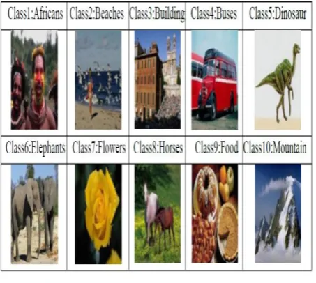
[image:6.595.320.539.54.245.2]A general-purpose WANG database is applied for content-based image retrieval (CBIR) system evaluation for testing holding 1000 core digital images in the format of JPEG with size (384x256 or 256x384). The database is built of 10 categories where each one contains a set of 100 images. In the implemented experiment, 10 images were randomly chosen where one image from each class. In this database, if the two images are from the same category, they considered a match. Particularly, a retrieved image is considered a match if and only if it is in the same class as the inquiry image. Fig. 12 presents a sample of Wang database images.
[image:6.595.311.542.310.730.2]Fig.12. Samples of the Wang database images. A query image is delivered by the user. Then related images from the database are selected and showed. For analysis purpose, a total of 10 assessment images are used to display the performance of the proposed system. These assessment images are shown in Fig. 13.
Fig. 13. The test images (query images). The query assessment image number 421.jpg of category ‘Dinosaur’ of the Wang database and 20 retrieved images from the database are displayed in Fig. 14. Also, the recovery results are explained in Fig. 15) for query image 666.jpg of the category ‘Flowers ’.
Fig. 14. The retrieved images from Wang database for the query image 421.jpg.
[image:6.595.55.282.497.700.2]To make a comparison on the retrieval performance, both the precision and recall are computed for the different number of retrieved images (N = 10, N = 20, N = 30, N = 40, N = 50, and N = 100) respectively. A large precision and recall value represent amazing performance for retrieval. The statistical results and performance are presented in Table- V and Fig. 16 for precision, and Fig. 17 for recall.
Table- V: The precision of different N retrieved images for each query images.
C la ss N a me Qu er y i ma g
e Precision (%)
N = 1 0 N = 2 0 N = 3 0 N = 4 0 N = 5 0 N = 1 0 0
Buses 339 100 95 96.6 97.5 88 90
Dinosaurs 421 100 100 100 100 98 93
Flowers 666 100 100 96.6 92.5 90 89
Horses 791 80 80 56 53.5 50 50
Africans 93 90 85 76 67.5 66 57
Monume nts
253 90 85 83.3 67.5 62 62
Foods 919 80 80 66.6 67.5 60 51
beaches 117 80 80 76.6 72.5 68 57
Elephants 522 50 40 30 35 38 43
Mountain s
879 60 55 53.3 43 48 51
Average precision
[image:7.595.50.289.158.715.2]83 80 73.5 69.65 66.8 64.3
Fig. 16. The precision of different N retrieved images for each query images
Fig. 17. The recall of N=100 retrieved images for each query images.
IV. CONCLUSION
An effective fusion structure was successfully constructed and demonstrated by combining two types of global image
features, the first one is the texture features of the image such as (Local Binary Pattern), while the second one is the shape features of the image such as (Edge Histogram Descriptor). The objective of this paper is how to construct a system that can be applied for locating the top n similar images for the query image in a suitable time. In this work, there are two reductions in size for image features. The first one is using LBP and EHD for representing images to 405 features regardless of the size of the image. While the second one is decreasing the 405 feature to only 6 features depend on the characteristic of SVD.
REFERENCES
1. Lowe, D. G, “Distinctive image features from scale-invariant keypoints”, International journal of computer vision, vol. 60, no.2, pp. 91-110.
2. Bay, H., Ess, A., Tuytelaars, T., & Van Gool, L, “Speeded-up robust features (SURF)”, J. Computer Vision and Image Understanding, vol. 110, no. 3, 2004, pp. 346-359,
3. VIMINA E R, “Computational Frameworks for Efficiency Enhancement of Content Based Image Retrieval Systems”, PhD. Dissertation in the Department of computer science, cochin university of science and technology, Kochi, India, 2017.
4. Swain, M. J., & Ballard, D. H, “ Color indexing”. International Journal of Computer Vision, vol. 7, no. 1, pp. 11-32.
5. Stricker & Orengo, “Similarity of colour images”, In IS&T/SPIE's Symposium on Electronic Imaging: Science & Technology, 1995, pp. 381-392.
6. Pass, G., & Zabih, R, “ Histogram refinement for content-based image retrieval”, In Proceedings 3rd IEEE Workshop on Applications of Computer Vision, 1996, pp. 96-102.
7. Huang, J., Kumar, S. R., Mitra, M., Zhu, W. J., & Zabih, R, “Image indexing using colorcorrelograms”, In Proceedings of the 1997 IEEE Computer Society Conference on Computer Vision and Pattern Recognition, 1997, pp. 762-768.
8. Kaplan, L. M., Murenzi, R., & Namuduri, K. R, “Fast texture database retrieval using extended fractal features”, In Proceedings of Photonics West'98 Electronic Imaging, 1997, pp. 162-173.
9. Haralick R. M., & Shanmugam K, “Textural features for image classification”, IEEE Transactions on Systems, Man, and Cybernetics, vol. 6, 1973, pp. 610-621.
10. Hervé N., & Boujemaa N., “Image annotation: which approach for realistic databases?”, In Proceedings of the sixth ACM international conference on Image and video retrieval, 2007, pp. 170-177. 11. Ngo C. W., Pong T. C., & Chin R. T. , “Exploiting image-indexing
techniques in DCT domain”, International Journal of Pattern Recognition, vol. 34, no. 9, 2011, pp. 1841-1851.
12. Suematsu N., Ishida Y., Hayashi A., &Kanbara, T, “Region-based image retrieval using wavelet transform” In Proceedings of the 15th international conf. on vision interface , 2002, pp. 9-16.
13. Neetesh Prajapati etl, “Edge Histogram Descriptor, Geometric Moment and Sobel Edge Detector Combined Features Based Object Recognition and Retrieval System”, International Journal of Computer Science and Information Technologies, vol. 7 , no. 1 , 2016, pp. 407-412.
14. Neil M., Lourenc M., and Herbst B. M., 2004," Singular Value Decomposition, Eigenfaces, and 3D Reconstructions", Society for Industrial and Applied Mathematics, vol. 46, no. 3, pp. 518–545 Assad Hussein Thary, “Satellite Image Classification Using K-Means and SVD Techniques”, Msc. Thesis in the College of Science / Al-Nahrain University, Iraq, 2016.
15. Yunshuang He and Guojun Lu and ShyhWei Teng, “An Investigation of Using K-d Tree to Improve Image Retrieval Efficiency”, DICTA2002: Digital Image Computing Techniques and Application, 21--22 January 2002, Melbourne, Australia.
16. Bentley, J. L.. "Multidimensional binary search trees used for associative searching". Communications of the ACM. Vol. 18 , no. 9, 1975, pp. 509–517. doi:10.1145/361002.361007
17. Jia Li, James Z. Wang, “Automatic linguistic indexing of pictures by a statistical modeling approach”,
Intelligence, vol. 25, no. 9,,2003, pp. 1075-1088.
18. Simardeep Kaur and Dr. Vijay Kumar Banga, “Content Based Image Retrieval: Survey and Comparison between RGB and HSV model”, International Journal of Engineering Trends and Technology (IJETT) – vol. 4, no. 4, 2013.
AUTHORSPROFILE
PhD. Student. Abdulkadhem Abdulkareem Abdulkadhem is a graduatestudent at the college of information technology, Department of software, university of Babylon, Iraq. He is currently pursuing his PhD. degree. AbdulKadhem holds a BS degree from the Department of computer science and MSc. Degree from the college of Information technology from university of Babylon. His research interests are primarily in multimedia, steganography and GIS.
Prof. Dr. Tawfiq A. Al-Assadi is a professor at the college of Information technology at the University of Babylon, Iraq. His research interests are primarily in Image processing, speech analysis, Genetic Algorithm., neural networks, information hiding, crypto-analysis, Finite Automata, Computer Graphics, Data Compression, GIS , Remote Sensing , Computer Viruses.