R E S E A R C H
Open Access
Spatial modulation based on
reconfigurable antennas: performance
evaluation by using the prototype of a
reconfigurable antenna
Dung Nguyen Viet
1, Marco Di Renzo
1*, Vedaprabhu Basavarajappa
2, Beatriz Bedia Exposito
2,
Jose Basterrechea
3and Dinh-Thuy Phan-Huy
4Abstract
In this paper, we study the performance of spatial modulation based on reconfigurable antennas. Two main
contributions are provided. We introduce an analytical framework to compute the error probability, which is shown to be accurate and useful for system optimization. We design and implement the prototype of a reconfigurable antenna that is specifically designed for application to spatial modulation and that provides multiple radiation patterns that are used to encode the information bits. By using the measured antenna radiation patterns, we show that spatial
modulation based on reconfigurable antennas works in practice and that its performance can be optimized by appropriately selecting the radiation patterns to use for a given data rate.
Keywords: Spatial modulation, Reconfigurable antennas, Antenna prototype, Error probability
1 Methods/experimental
The methods used in the paper are based on mathematical tools and theories. A new analytical framework for perfor-mance analysis is introduced. The theoretical framework is validated against Monte Carlo simulations, by using empirical data.
2 Introduction
Spatial modulation (SM) [1] is a promising low-complexity [2] and energy-efficient [3] multiple-antenna modulation scheme, which is considered to be espe-cially suitable for application to the Internet of Things (IoT) [4]. For these reasons, SM has attracted the atten-tion of several academic and industrial researchers [5]. A comprehensive description of the main achievements and latest developments on SM research can be found in [6–10]. Some pioneering and recent experimental activi-ties can be found in [11–14]. The research literature on
*Correspondence:[email protected]
1Laboratoire des Signaux et Systèmes, CNRS, CentraleSupelec, Univ Paris-Sud,
Université Paris-Saclay, Plateau du Moulon, 91192 Gif-sur-Yvette, France Full list of author information is available at the end of the article
SM is vast, and various issues have been tackled during the last few years, which include the analysis of the error prob-ability [15], the design and analysis of transmit-diversity schemes [16,17], and the analysis and optimization of the achievable rate [18,19]. A recent comprehensive literature survey on SM and its generalizations is available in [10].
Among the many SM schemes that have been proposed in the literature, an implementation that is suitable for IoT applications is SM based on reconfigurable anten-nas (RectAnt-SM) [20]. In SM, the information bits are encoded onto the indices of the antenna elements of a given antenna array. In RectAnt-SM, by contrast, the information bits are encoded onto the radiation patterns (RPs) of a single-RF and reconfigurable antenna. This implementation has several advantages, especially for IoT applications [4].
In spite of the potential applications of RectAnt-SM in future wireless networks, to the best of the authors’ knowl-edge, no analytical framework for computing the error probability of this emerging transmission technology is
available. In the present paper, motivated by these consid-erations, we introduce an analytical framework that allows us to estimate the performance and to optimize the oper-ation of RectAnt-SM. We prove, in particular, that the diversity order of RectAnt-SM is the same as the diversity order of SM, which coincides with the number of antennas at the receiver.
In order to substantiate the practical implementation and performance of RectAnt-SM, we design a single-RF and reconfigurable antenna that provides us with eight different RPs for encoding the information bits at a low-complexity and high energy efficiency. The proposed antenna is designed, and a prototype is implemented and measured in an anechoic chamber. Based on the man-ufactured prototype, we employ the measured RPs to evaluate the performance of RectAnt-SM. With the aid of our proposed analytical framework, in particular, we show that the error probability can be improved by appropri-ately choosing the best RPs, among those available, that minimize the average bit error probability.
Together with [4], the results contained in the present paper constitute the first validation of the performance of RectAnt-SM by using a realistic reconfigurable antenna that is capable of generating multiple RPs with adequate spatial characteristics for modulating information bits.
The remainder of the present paper is organized as fol-lows. In Section 3, the system model is introduced. In Section4, the analytical framework of the error probabil-ity is described. In Section5, the prototype of the single-RF and reconfigurable antenna is presented. In Section6, numerical results are illustrated, and the performance of RectAnt-SM is analyzed. Finally, Section7concludes the paper.
Notation: We adopt the following notation. Matrices, vectors, and scalars are denoted by boldface upper-case (e.g., A), boldface lowercase (e.g.,a), and lowercase respectively (e.g.,a). The element(u,v)of a matrix Ais denoted byAu,v, and theuth entry of a vectorais denoted by au. The transpose, complex conjugate, and complex conjugate transpose ofAare denoted byAT ,A∗, andAH
respectively. The absolute value of a complex numbera is defined by|a|.Ea{·}andEA{·}denote the expectation operator of random variableaand matrixA, respectively. j = √−1 is the imaginary unit. Pr{·}denotes probabil-ity.·· denotes the binomial coefficient. TheQ-function
is defined as Q(x) = 1/√2π x∞exp
−u2 2
du. The moment generating function (MGF) of random variableX is defined asMX(s)=EX{exp(−sX)}. The gamma func-tion is defined as (z) = 0∞xz−1e−xdx. The modified Bessel function of order zero is defined asI0(·).
3 System model
In this section, we introduce the signal model, the channel model, and the demodulator.
3.1 Signal model
Let us consider aNr×Ntmultiple-input-multiple-output (MIMO) system that use aM-ary signal constellation dia-gram. In a conventional SM transmission scheme [1], the data stream is divided into two blocks, where the first block of log2(Nt)bits is used to identify the index of the transmitted antenna and log2(M)bits are used to identify a symbol of the signal constellation diagram. By assum-ing that channel state information (CSI) is known at the receiver, the objective of the detector is to jointly estimate the active antenna and the data symbol that is transmitted in order to retrieve the entire transmitted bitstream.
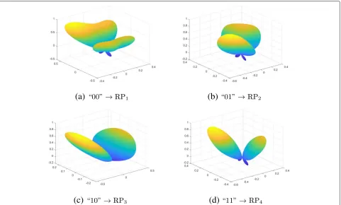
Let us now consider the RecAnt-SM transmission scheme. In this case, we consider that the transmitter is equipped with a reconfigurable antenna that is capable of generatingPdifferent RPs. In this case, the RP that is used for transmission is also used to encode the informa-tion, in addition to the signal constellation diagram [20]. More precisely, the joint combination of antenna’s RP and channel constitutes the physical resource that is used to encode the information bits. IfP RPs are available, then log2(P)+log2(M)bits of information can be transmitted. Compared with conventional SM, RecAnt-SM has the advantage of not requiring an array of antennas to enhance the data rate. In addition, RecAnt-SM can be implemented at a low cost, by using simple and compact antennas, where different RPs can be obtained by realiz-ing appropriate circuits that modify the current flowrealiz-ing through the physical antenna. These specific features of RectAnt-SM make it useful for IoT applications. In the sequel, we will discuss an antenna that we have designed and fabricated and that allows us to implement RectAnt-SM in practice. As an example, let us considerP=M=4. Then, log2(P) = 2 bits are used to identify the RP and log2(M) = 2 are used to identify a symbol of the signal constellation diagram. Figure1illustrates a simple exam-ple of the imexam-plementation of RectAnt-SM, by focusing only on the RPs, e.g., RectAnt-SSK (space shift keying).
Let us assume that thepth RP and the symbolxm are selected based on information bits to be transmitted. The Nr×1 received signal vector can be formulated as follows:
y=√ρHepxm+w (1)
(a)
(b)
(c)
(d)
Fig. 1 a–dIllustration of RecAnt-SSK withP=4. The RPs are obtained from a designed and manufactured antenna that is described in the sequel
RecAnt-SSK constitutes a special case of RecAnt-SM, where the information bits are encoded only into the RPs. In this case, the signal model simplifies as follows:
y=√ρHep+n (2)
Based on the signal model in (1), the maximum likeli-hood (ML-) optimum demodulator, by assuming full CSI available at the receiver, can be formulated as follows [2]:
q,x n
= arg max
forq=1,...,Pandn=1,...,M
D(q,xn)
(3)
where:
D(q,xn)= Nr
nr=1
y∗nrHnr,qxn
−1
2Hnr,qxn
2 (4)
whereynr is thenrth entry ofyandHnr,qthe entry in the
rownr and columnqofH. The demodulator of RectAnt-SSK can be obtained in a similar way.
3.2 Channel model
In this section, we introduce the channel modelHthat we briefly mentioned in the previous section. As far as RectAnt-SM is concerned, the channel model plays an important role, since the combined effect of RP and chan-nel determines the system performance. Since we consider three-dimensional RPs (see Fig.1), the considered channel
model is chosen appropriately. More precisely, the chan-nel model is based on a ray-based and cluster approach similar to [21]. A sketched representation of the channel model is given in Fig.2.
For simplicity and without loss of generality, we con-sider a channel model with a single cluster and with multiple rays. The number of rays is denoted byK. The Nr × P channel matrix, which accounts for the RPs of the reconfigurable antenna as well, can be formulated as follows:
H= √1
K K
k=1
βkar
θr k,φkr at
θt k,φkt
T
(5)
where the normalization factor 1/√Kpreserves the aver-age unit energy of the channel, and the following notation is used:
• βkis the fading coefficient of thek th ray;
• aris theNr×1array response vector of the receiver;
• atis theNt×1array response vector of the transmitter;
• θt k,φtk
are the azimuth and elevation angles of departure (AoD) of thek th ray; and
• θr k,φkr
Fig. 2Sketched representation of the channel model
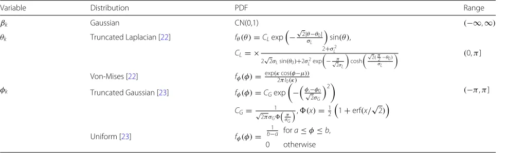
As far as the statistical distributions ofβk,θk, andφkas concerned, Table1summarizes the most commonly used models. In particular,θk is often modeled as a truncated Laplacian random variable, and φk is often modeled as a Von-Mises, truncated Gaussian, or an uniform random variable. For each ray, the random variables are assumed to be independent and identically distributed.
The specific characteristics of the receiver and trans-mitter are determined byarandat, respectively. As far as the receiver is concerned, we consider, as an example, a uniform linear array with an onmi-directional RP of unit gain. As far as the transmitter is concerned, we consider a reconfigurable antenna withPdifferent RPs. The RPs are denoted as follows:
Gp(θ,φ)=
Gp(θ,φ)exp
jp(θ,φ)
(6)
for p = 1,. . .,P, and Gp(θ,φ) and p(θ,φ) are the amplitude and phase of thepth RP, respectively.
Based on these assumptions,Hnr,pcan be formulated as
follows:
Hnr,p=
1
√
K K
k=1
βkexp(jkd(nr−1)sin(θkr)sin(φkr)) Receiver part
×
Gp(θkt,φkt)exp(jp(θkt,φkt))
Transmitter part
(7)
where nr = 1,. . .,Nr, p = 1,. . .,P, d is the distance between adjacent antennas, andk(θ,φ)is the wavevector defined as follows:
k(θ,φ)= 2π
λ [sin(θ)cos(φ), sin(θ)sin(φ), cos(θ)]T (8)
whereλis the wavelength.
4 Average bit error probability
From [15], it is known that the average bit error proba-bility (ABEP) of the system model under analysis can be formulated as follows:
ABEP≤ 1 PM
1 log2(PM)
P
p=1 M
m=1 P
q=1 M
n=1
NHAPEP((p,xm)→(q,xn))
(9)
where APEP denotes the average pairwise error probabil-ity, which is the probability of demodulating the RPqand the symbolxn if the RPpand the symbol xm have been transmitted and are the only two possible options, andNH denotes the number of bits that the latter two constellation points different from each other.
The pairwise error probability (PEP), PrE, of deciding for the qth radiation pattern while the pth radiation pattern is transmitted and deciding for the symbol xn
Table 1Distribution of variables for the considered channel model
Variable Distribution PDF Range
βk Gaussian CN(0,1) (−∞,∞)
θk Truncated Laplacian [22] fθ(θ)=CLexp
−√2|θ−θ0|
σL
sin(θ),
CL= × 2+σ
2
L 2√2σLsin(θ0)+2σL2exp
−√π
2σL
cosh √
2( π2−θ0) σL
(0,π]
φk
Von-Mises [22] fφ(φ)=exp(κ2πcosI(φ−μ)) 0(κ)
(−π,π] Truncated Gaussian [23] fφ(φ)=CGexp
−φ√,−φ0
2σG 2
CG= √ 1
2πσG π
σG
,(x)= 121+erf(x/√2)
Uniform [23] fφ(φ)=
1
b−a fora≤φ≤b,
while the symbol xm is transmitted can be written as follows:
PrE((p,xm)→(q,xn)|H)=Pr(D(p,xm) <D(q,xn))
=Q
ρ
2γp,q,xm,xn(H)
(10)
where:
γp,q,xm,xn(H)=
Nr
nr=1
Hnr,qxn−Hnr,pxm
2
(11)
As a result, the APEP can be written as follows:
APEP((p,xm)→(q,xn))
=EH
Q
ρ
2γp,q,xm,xn(H)
(a)
=EH
1
π
π/2
0 exp
−ργ p,q,xm,xn
4sin2(ϑ)
dϑ
(b)
= 1 π
π/2
0
Mγp,q,xm,xn
−ρ
4sin2(ϑ)
dϑ (12)
where (a) and (b) follow by applying Craig’s formula [15] and from the definition of MGF ofγp,q,xm,xn, respectively.
4.1 Setup withNr=1
We start by considering the system setup with Nr = 1. The APEP is formulated in the following proposition.
Proposition 1Letζ (¯ K,ϑ) = 4Ksinρ2(ϑ). If Nr = 1, the APEP of RecAnt-SM is as follows:
APEP=
1
π
π/2
0
∞
0
exp(−z)
π
0
π
−πexp
−zζ (¯ K,ϑ)
ψp,q,xm,xn,θt,φt
fθθtfφφtdθtdφt K
dz dϑ
(13)
where
ψp,q,xm,xn,θt,φt
=Gq
θt,φtexpjqθt,φtx n
−Gp(θt,φt)exp(jp(θt,φt))xm 2
(14)
ProofSee theAppendix.
In the high-SNR regime, the APEP is given in the follow-ing proposition.
Proposition 2If Nr =1, the APEP of RecAnt-SM in the
high-SNR regime is as follows:
APEP≤1
ρ
∞
0
π
0
π
−πexp
−z1 Kψ
p,q,xm,xn,θt,φt
fθ(θt)fφ(φt)dθtdφtK dz
(15)
whereψis defined in (14).
ProofSee theAppendix.
Equations (13) and (15) provide one with accurate per-formance predictions of the APEP. The analytical expres-sion is, however, quite complex due to the discrete number of rays that are considered in the system model. In the following two propositions, we provide an asymptotic expression of the APEP under the assumptionK → ∞. In the sequel, we will show that the simplified analyti-cal expression of the APEP is accurate even for moderate values ofK.
Proposition 3Assume K→ ∞and Nr=1. The APEP
can be simplified as follows:
APEP≤1
2
1−
ρ ρ+4
(16)
where
=
π
0
π
−πψ
p,q,xm,xn,θt,φtfθ(θt)fφ(φt)dθtdφt
(17)
whereψis defined in (14).
ProofSee theAppendix.
Proposition 4Assume K→ ∞and Nr=1. The APEP
in the high-SNR regime can be simplified as follows:
APEP≤ 1
ρ (18)
whereis defined in (17).
ProofSee theAppendix.
4.2 Setup withNr=2
In this section, we study the system setup where two antennas are available at the receiver. The following proposition generalizes Proposition3
Proposition 5Assume K → ∞and Nr =2. The APEP
in the high-SNR regime can be formulated as follows:
APEP≤
3
ρ2π
−π π
0ψ
p,q,xm,xn,θt,φt
fθ(θt)fφ(φt)dθtdφt2
=1−−ππ0πcos(kd(sin(θr)sin(φr))) fθ(θr)fφ(φr)dθrdφr2−
π
−π π
0 sin(kd(sin(θr)sin(φr))) fθ(θr)f
φ(φr)dθrdφr2
(19)
whereψis defined in (14).
By direct inspection of the obtained APEP, we evince that the diversity order is equal to two if two anten-nas are available at the receiver. This is consistent with conventional SM [15].
4.3 Setup with genericNr
In this section, we generalize the previous analytical frameworks for Nr = 1 andNr = 2, by considering a generic value ofNr.
Fig. 3Fabricated antenna for implementing RectAnt-SM
Theorem 1 Assume K→ ∞. The APEP in the high-SNR
regime can be formulated as follows:
APEP≤
αNr
ρNrψp,q,xm,xn,θt,φtNrEθr,φr Fθ1,r,. . .,θNr,r,φ1,r,. . .,φNr,r
αNr= 1 2
2Nr
Nr
+ Nr−1
k=0
(−1)Nr−k2
2Nr
k
sin(π (Nr−k))
2π (Nr−k)
(20)
whereψis defined in (14).
Proof See theAppendix.
By direct inspection of the obtained APEP, we observe that the diversity order is equal toNr, as in conventional SM [15].
The main limitation of (20) is that
Eθr,φr Fθ1,r,. . .,θNr,r,φ1,r,. . .,φNr,r is not
analyt-ically tractable and cannot, in general, be formulated in closed-form. In some special cases, however, this is possible, notably ifNr = 3, as reported in the following proposition.
Proposition 6Assume K → ∞and Nr =3. The APEP
in the high-SNR regime can be formulated as follows:
APEP≤
10 ρ3ψp,q,xm,xn,θt,φt3Eθr
,φr Fθ1,r,θ2,r,θ3,r,φ1,r,φ2,r,φ3,r
(21)
where the following definition holds true:
Eθr,φr Fθ1,r,θ2,r,θ3,r,φ1,r,φ2,r,φ3,r=
1+2(E1)2E3−2(E2)2E3+4E1E2E4−(E3)2
−(E4)2−2(E1)2−2(E2)2
(22)
with
E1=
π
−π
π
0
coskdsinθrsinφr
fθθrfφφrdθrdφr (23)
E2=
π
−π
π
0
sinkdsinθrsinφr
fθθrfφφrdθrdφr (24)
E3=
π
−π
π
0
cos2kdsinθrsinφr
fθθrfφφrdθrdφr (25)
E4=
π
−π
π
0
sin2kdsinθrsinφr
fθθrfφφrdθrdφr (26)
ProofSee theAppendix.
Fig. 5Measurement of the antenna prototype in an anechoic chamber
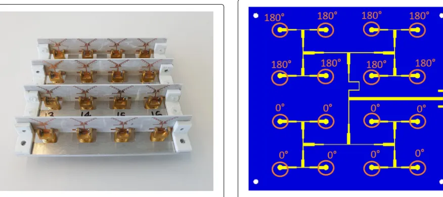
5 Antenna prototype with reconfigurable radiation patterns
In order to test the performance of RectAnt-SM and to assess its practical feasibility, we have designed and fabricated a reconfigurable antenna that yields multiple radiation patterns. A photo of the antenna prototype specifically designed to implement RectAnt-SM is given in Fig.3. The proposed antenna needs a single radio fre-quency chain and is capable of generating eight RPs. Four of them are illustrated in Fig.1. The eight different RPs are obtained by considering a 4× 4 array, as illustrated in Fig.4, and by using a different excitation matrix. Five excitation matrices are reported as follows:
⎡ ⎢ ⎢ ⎣
0 + + 0 0 + + 0 0 − − 0 0 − − 0
⎤ ⎥ ⎥ ⎦
A ,
⎡ ⎢ ⎢ ⎣
0 0 + +
0 0 + +
− − 0 0
− − 0 0 ⎤ ⎥ ⎥ ⎦
B ,
⎡ ⎢ ⎢ ⎣
0 0 0 0
− − + + − − + +
0 0 0 0 ⎤ ⎥ ⎥ ⎦
C ,
⎡ ⎢ ⎢ ⎣
− − 0 0
− − 0 0
0 0 + +
0 0 + +
⎤ ⎥ ⎥ ⎦
D ,
⎡ ⎢ ⎢ ⎣
0 − − 0 0 − − 0 0 + + 0 0 + + 0
⎤ ⎥ ⎥ ⎦
E
(27)
Each entry of the 4×4 matrix represents the excitation that is fed into the corresponding antenna of the array. The excitation has unit amplitude, and its phase is either 0 or 180, which is denoted by the sign “+” and “−”, respectively, in the excitation matrices.
The designed prototype has been studied and optimized by simulating the 4×4 antenna array with the full-wave solver Ansys HFSS. Based on the optimized design, a pro-totype antenna has been fabricated and its RPs have been measured in an anechoic chamber, as illustrated in Fig.5.
-50
0
50
-60
-50
-40
-30
-20
-10
0
-5 0 5 10 15 20 25 30 35 40 10-4
10-3 10-2 10-1 100 101 102
Fig. 7ABEP of RecAnt-SM (P=2,Nr=1,M=2 (BPSK)). The results are obtained by using RP1and RP2
In Fig. 6, we report, as an example, the simulated and measured RP RP1that is reported in Fig.1as well.
6 Numerical results and discussion
In this section, we provide some numerical results in order to validate the analytical derivation of the bit error prob-ability and in order to asses the achievable performance
by using the RPs that are obtained from the fabricated antenna prototype. We show, in particular, that by appro-priately selecting the RPs that minimize the analytical framework of the error probability, the error probability can be greatly decreased.
In Fig. 7, we compare Monte Carlo simulations against the proposed analytical framework of the bit
-5 0 5 10 15 20 25 30 35 40
10-4 10-3 10-2 10-1 100 101 102
29 30 31
0.005 0.01 0.015 0.02
15 20 25 30 35 40 10-6
10-5 10-4 10-3 10-2 10-1 100
Fig. 9ABEP of RecAnt-SM (P=2,Nr=1, 2, 3,M=2 (BPSK)). The results are obtained by using RP1and RP2
error probability. In Fig. 8, we study the impact of K on the error probability with the aim of assessing the accuracy of the asymptotic framework for K →
∞. Both figures confirm that our analytical frame-works are accurate and in agreement with Monte Carlo simulations.
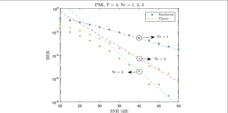
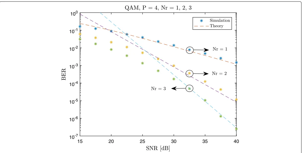
In Figs.9,10, and11, we report the bit error probability as a function of the number of antennas at the receiver. We observe the good accuracy of the proposed analytical frameworks, and we note, in particular, that RectAnt-SM provides one with a diversity order equal to the number of antennas at the receiver.
20 25 30 35 40 45 50
10-8 10-6 10-4 10-2 100
15 20 25 30 35 40 10-7
10-6 10-5 10-4 10-3 10-2 10-1 100
Fig. 11ABEP of RecAnt-SM (P=4,Nr=1, 2, 3,M=4 (QPSK)). The results are obtained by using RP1-RP4
In Fig.12, we report the APEP as a function of the RPs. In particular, with the aid of the analytical framework of the error probability, we compute the ABEP for all pos-sible combinations of four out of eight RPs in order to identify the impact of the RPs on the error performance. We observe that an appropriate choice of the RPs can yield a significant performance gain. The reason is that, due to practical design constraints, it may not be possi-ble to design several RPs that are very different from each other. Therefore, identifying the best of them that provide good performance as a function of the channel model is an important optimization problem. The proposed analytical
framework allows us to solve this optimization problem at a low complexity and high efficiency.
7 Conclusion
In this paper, we have studied the performance of spa-tial modulation based on reconfigurable antennas. We have introduced an analytical framework to compute the error probability and have described the prototype of a reconfigurable antenna that is specifically designed for application to spatial modulation. By using the radiation patterns obtained from the manufactured antenna pro-totype, we have shown that spatial modulation based on
Fig. 12ABEP of RecAnt-SSK (P=4,Nr=3). The different markers show the ABEP by choosing four RPs out of eight RPs in order to identify those
reconfigurable antennas works in practice and that its per-formance can be optimized by appropriately choosing the radiation patterns that minimize the proposed analytical framework of the error probability.
Appendix
Proof of Proposition1
Letνnr =Hnr,qxn−Hnr,pxmfornr=1,. . .,Nr. Recall that
Nr=1. We note thatν1is a zero mean complex Gaussian variable with variance:
σ2
whose probability density function is:
fx(x;λ)=λexp(−λx), x0
withλ=1/σ2 ν1.
The APEP can then be formulated as follows:
APEP= 1
We note that σν21 is a random variable that depends on
θt k,φkt
K
k=1. The expectation can be computed by using the approach introduced in [24], as follows:
APEP= 1
With the aid of some algebraic manipulations, we obtain the following:
The proof follows from the following identity:
π
Proof of Proposition2
From (29), we obtain, in the high-SNR regime, the following:
The rest of the proof follows by using similar steps as for the proof of Proposition1.
Proof of Proposition3
By using the Maclaurin series expansion and keeping the first two dominant terms, we have the following:
By using this approximation, we have the following:
Let us consider the following integral:
=
In addition, the following holds true:
lim
where we used the following notable limit:
lim
Therefore, the asymptotic APEP is:
APEP≤1
where the first equality (a) comes from the fact that
∞
0 exp(−zc)=1c,c > 0 and the second equality (b) follows from (5A.4a) in [25]. This concludes the proof.
Proof of Proposition4
By using steps similar to Proposition 3, the asymptotic APEP can be written as follows:
APEP≤ 1
which concludes the proof.
Proof of Proposition5
We first introduce the following lemma [26] for appli-cation to hermitian quadratic forms in complex normal variables.
Lemma 1Let vn(n = 1,. . .,N) be a set of complex Gaussian random variables having zero mean. Letκ, with
v=[v1,· · ·,vN]T, be an Hermitian quadratic form:
κ=vHINv (42)
Its MGF is as follows:
Mκ(s)= N +
n=1
(1−sλn)−1 (43)
whereλn is the nth eigenvalue of the covariance matrix
Rv=E{vvH}.
Proof See [26].
The proof of Proposition5can be split in three steps.
Step 1: By using Lemma1withN=Nr=2, we have:
whereλ1andλ2are eigenvectors of the covariance matrix:
R=
andRis assumed to be full rank.
It is worth mentioning thatλ1andλ2depend on the ran-dom variablesθkt,φtk,θkr,φkr. In particular, from Lemma1,
Also, we have the following:
For high SNR, we have:
where we have used the second-order Taylor approxima-tion.
where (a) follows from:
1
Step 2: We compute the explicit expression of the product
λ1λ2. To this end, we introduce the following lemma.
Lemma 2Assume thatR, defined in (45), is full rank
and has two distinct eigenvaluesλ1andλ2. The product of the two eigenvectorsλ1andλ2is as follows:
λ1λ2=Eθt,φt,θr
ProofBy definition:
ν1=
Moreover, it is known that the product of the eigenval-ues is equal to the determinant of the covariance matrix (i.e., det(R)=λ1λ2). Thus,λ1λ2can be computed directly where we have used the identity:
expjφ+exp−jφ
Step 3:We exploit the asymptotic analysis introduced in Proposition3to derive a closed-form expression of the APEP. We apply the following formula that is a special case of (40) in [24] forX=λ1λ2: Then, we obtain:
where the last equality follows from the assumption of independent and identically distributed random variables.
Moreover, by using the following approximation:
exp we conclude the proof by using the following result:
π
Proof of Theorem 1
The proof of Theorem1generalizes the steps of Proposi-tion5as follows.
Step 1: From Lemma1, we have:
Then, we need to identify the coefficients Anr
Nr
nr=1so that the following is satisfied:
1
To this end, we can exploit the general formula of partial fraction decomposition [pp. 66–67], [27]:
Anr = Thus, we have:
APEP≈Eθt,φt,θr,φr
In the high SNR regime, we can use the Nrth-order Taylor approximation as follows:
We note that the following holds true:
1
sin2m(ϑ)= 1
Let us define:
αm=
Then, we have the following:
APEP≈Eθt
By induction, the following can be proved:
Nr
of Lemma2, we obtain the following:
det(Rv)= Step 3: The APEP is then the following:
EX{exp(Xz)}
By using the following approximation:
we have:
Thus, we obtain:
αNr
This concludes the proof.
Proof of Proposition5
From Theorem1, we can obtain (21). We need to prove how to obtain the explicit form of the function F(·). If Nr = 3, the determinant of the covariance matrixRcan be computed as follows:
det(R)=
We note that:
E νuνv∗
which can be further simplified as follows:
Fθr
where we have used similar observations as forNr =2.
Now, we need to compute
By applying the following trigonometric identities:
cos(a+b−2c)=cos(a)cos(b)cos(2c)
−sin(a)sin(b)cos(2c)+sin(a)cos(b)sin(2c)
+sin(b)cos(a)sin(2c)
cos(c+b−2a)=cos(c)cos(b)cos(2a)
−sin(c)sin(b)cos(2a)+sin(c)cos(b)sin(2a)
+sin(b)cos(c)sin(2a)
(86)
and noting thata,b, andcare independent, we eventually obtain the desired result after some algebraic manipula-tions.
Funding Not applicable.
Availability of data and materials
Data sharing is not applicable to this article as no datasets were generated or analyzed during the current study. The paper is built upon mathematical analysis and experimental validation.
Authors’ contributions
The authors declare that they have equally contributed to the paper. All authors read and approved the final manuscript.
Competing interests
The authors declare that they have no competing interests.
Publisher’s Note
Springer Nature remains neutral with regard to jurisdictional claims in published maps and institutional affiliations.
Author details
1Laboratoire des Signaux et Systèmes, CNRS, CentraleSupelec, Univ Paris-Sud,
Université Paris-Saclay, Plateau du Moulon, 91192 Gif-sur-Yvette, France.2TTI
Norte, Parque Cientifico y Tecnologico de Cantabria, Albert Einstein 14, 39011 Santander, Cantabria,Spain.3University of Cantabria, Av. de los Castros, s/n,
39005 Santander, Cantabria, Spain.4Orange Labs, Orange Gardens, 44 avenue
de la Republique, CS 50010, 92326 Chatillon Cedex, France.
Received: 28 December 2018 Accepted: 10 April 2019
References
1. M. Di Renzo, H. Haas, P. M. Grant, Spatial modulation for multiple-antenna wireless systems: a survey. IEEE Commun. Mag.49(12), 182–191 (2011) 2. A. Younis, S. Sinanovic, M. Di Renzo, R. Y. Mesleh, H. Haas, Generalised
sphere decoding for spatial modulation. IEEE Trans. Commun.61(7), 2805–2815 (2013)
3. A. Stavridis, S. Sinanovic, M. Di Renzo, H. Haas, in2013 IEEE 78th Vehicular Technology Conference (VTC Fall). Energy evaluation of spatial modulation at a multi-antenna base station (IEEE, Las Vegas, 2013), pp. 1–5.https:// doi.org/10.1109/VTCFall.2013.6692187
4. D.-T. Phan-Huy, et al., Single-carrier spatial modulation for the Internet of Things: design and performance evaluation by using real compact and reconfigurable antennas, submitted (2018).https://arxiv.org/abs/1812. 07514.https://doi.org/10.1109/ACCESS.2019.2895754
5. P. Patcharamaneepakorn, S. Wu, C.-X. Wang, E.-H. M. Aggoune, M. M. Alwakeel, X. Ge, M. Di Renzo, Spectral, energy, and economic efficiency of 5G multicell massive MIMO systems with generalized spatial modulation. IEEE Trans. Veh. Technol.65(12), 9715–9731 (2016)
6. M. Di Renzo, H. Haas, A. Ghrayeb, S. Sugiura, L. Hanzo, Spatial modulation for generalized MIMO: challenges, opportunities and implementation. Proc. IEEE.102(1), 56–103 (2014)
7. P. Yang, M. Di Renzo, Y. Xiao, S. Li, L. Hanzo, Design guidelines for spatial modulation. IEEE Commun. Surv. Tuts.16(1), 6-26 (2015)
8. P. Yang, Y. Xiao, Y. L. Guan, K. V. S. Hari, A. Chockalingam, S. Sugiura, H. Haas, M. Di Renzo, C. Masouros, Z. Liu, L. Xiao, S. Li, L. Hanzo, Single-carrier SM-MIMO: a promising design for broadband large-scale antenna systems. IEEE Commun. Surv. Tuts.18(3), 1687-1716 (2016) 9. M. Di Renzo, H. Haas, A. Ghrayeb, L. Hanzo, S. Sugiura, inWiley
Encyclopedia of Electrical and Electronics Engineering. Spatial Modulation for Multiple-Antenna Communication, (2016).https://doi.org/10.1002/ 047134608X.W8327
10. E. Basar, M. Wen, R. Mesleh, M. Di Renzo, Y. Xiao, H. Haas, Index modulation techniques for next-generation wireless networks. IEEE Access.5, 16693–16746 (2017).https://doi.org/10.1109/ACCESS.2017.2737528 11. A. Younis, W. Thompson, M. Di Renzo, C.-X. Wang, M. A. Beach, H. Haas,
P. M. Grant, Performance of spatial modulation using measured real-world channels. IEEE Veh. Technol. Conf. - Fall, 1–5 (2013) 12. N. Serafimovski, A. Younis, R. Mesleh, P. Chambers, M. Di Renzo, C.-X.
Wang, P. M. Grant, M. A. Beach, H. Haas, Practical implementation of spatial modulation. IEEE Trans. Veh. Technol.62(9), 4511–4523 (2013) 13. P. Liu, M. Di Renzo, A. Springer, Line-of-sight spatial modulation for indoor
mmWave communication at 60 GHz. IEEE Trans. Wirel. Commun.15(11), 7373–7389 (2016)
14. P. Liu, J. Blumenstein, N. S. Perovic, M. Di Renzo, A. Springer, Performance of generalized spatial modulation MIMO over measured 60 GHz indoor channels. IEEE Trans. Commun.66(1), 133–148 (2018)
15. M. Di Renzo, H. Haas, Bit error probability of SM-MIMO over generalized fading channels. IEEE Trans. Veh. Technol.61(3), 1124–1144 (2012) 16. M. Di Renzo, H. Haas, On transmit-diversity for spatial modulation MIMO:
impact of spatial-constellation diagram and shaping filters at the transmitter. IEEE Trans. Veh. Technol.62(6), 2507–2531 (2013) 17. M.-T. Le, V.-D. Ngo, H.-A. Mai, X.-N. Tran, M. Di Renzo, Spatially modulated
orthogonal space-time block codes with nonvanishing determinants. IEEE Trans. Commun.62(1), 85–99 (2014)
18. D. A. Basnayaka, M. Di Renzo, H. Haas, Massive but few active MIMO. IEEE Trans. Veh. Technol.65(9), 6861–6877 (2016)
19. N. S. Perovic, P. Liu, J. Blumenstein, M. Di Renzo, A. Springer, Optimization of the cut-off rate of generalized spatial modulation with transmit precoding. IEEE Trans. Commun.66(10), 4578–4595 (2018)
20. M. Di Renzo, Spatial modulation based on reconfigurable antennas - a new air interface for the IoT. IEEE Mil. Commun. Conf., 1–6 (2017) 21. Q. U. A. Nadeem, A. Kammoun, M. Debbahn, M. S. Alouini, A generalized
spatial correlation model for 3D MIMO channels based on the Fourier coefficients of power spectrums. IEEE Trans. Sig. Proc.63(14), 3671–3686 (2015)
22. J. Zhang, C. Pan, F. Pei, G. Liu, X. Cheng, Three-dimensional fading channel models: a survey of elevation angle research. IEEE Commun. Mag.52(6), 218–226 (2014)
23. T. S. Pollock, T. D. Abhayapala, R. A. Kennedy, Three-dimensional fading channel models: a survey of elevation angle research. Telecommun. Syst. 24(2), 415–436 (2003)
24. M. Di Renzo, C. Merola, A. Guidotti, F. Santucci, G. E. Corazza, Error performance of multi-antenna receivers in a Poisson field of interferers: a stochastic geometry approach. IEEE Trans. Commun.61(5), 2025–2047 (2013)
25. M.K. Simon, M.-S. Alouini,Digital Communication over Fading Channels. (Wiley, 2005)
26. G.L. Turin, The characteristic function of Hermitian quadratic forms in complex normal variables. Biometrika.67(1/2), 199–201 (1960) 27. A. Jeffrey, D. Zwillinger,Table of Integrals, Series, and Products. (Elsevier,