Abstract: While taking an MRI scan, the patients cannot static for a long time during the motions; the image formation process can create artifacts that may reduce the image quality. The Compressed Sensing (CS) mechanism is employed to reconstruct the original image from the limited data given as the sparse matrix. Hence, CS can be utilized to reduce the acceleration time for an MRI scan considering the patient's health. So the sensing method is implemented by a suitable projection matrix for reconstructing the sparse signals from a few numbers of measurements using Compressed Sensing. The CS guarantees the recovery of the original image with high probability based on random Gaussian projection matrices. However, sparse ternarius projections are more apt for the implementation of hardware. In this article, the proposed deep learning method is employed to obtain a very sparse ternary projection in Compressed Sensing. Compressed Sensing Reconstruction using an adaptive scale parameter based on the texture feature is used to improve the image quality. The two scaling factors αx and αy are assigned to specify the fixed scale for changing the improvement of the image quality. In the parameter using texture feature, the αx and αy are assigned to α as an adaptive scale based on texture feature. In the TACS-SDANN architecture, there are two layers namely the sensing layer which trains the projection matrix and a reconstruction layer which trains for non-linear sparse matrix continuously using Auto-encoder. Experimentally, the scaling factors are calculated on the training data to get the mean Peak-Signal-to-Noise Ratio (PSNR) for improving the image quality. Hence a new deep network layer is employed to improve the image quality in this proposed method. Hence the consequence of the proposed method is compared with the SDANN method based on the mean Peak-Signal-to-Noise Ratio (PSNR) to check the image quality. From that comparisons, the TACS-SDANN architecture is proposed to yield a better performance.
Keywords: Compressed Sensing, Deep Learning, SDANN architecture, LBP image, Sparse-LBP ternary projection.
I. INTRODUCTION
CS joins compression and sensing or acquisition. Here sparsity is used for recovering the signals that have been sampled at a significantly lower frequency than the requirements of the Shanon/Nyquist theorem [1]. In medical regions such as MRI and CT, audio or video or image [2], the effective processing and analysis of high-dimensional data using CS are very important.
Consider the compressed representation of the testing signal x ϵ Rn is detained by CS using sensing mechanism.
Revised Manuscript Received on October 05, 2019.
*Correspondence author
D.M.Annie Brighty Christilin* Research Scholar, Manonmaniam Sundaranar University, Tirunelveli. [email protected]
Dr.M.Safish Mary Assistant Professor, Department of Computer Science, St.Xaviers College, Tirunelveli. [email protected]
It is examined by sensing or projection matrix. Instead of pixels, the linear measurements are taken as given below:
y1=<x, Φ1> y2=<x, Φ2> … ym=<x,Φm> y=Φ x (1)
Where Φ ϵ R m x n
In R m x n, m x n is the projection matrix. y ϵ Rm is the vector that contains the acquired measurements. In Sparse Sampling, let assume either x is a sparse signal or x has a sparse representation for a suitable basis ψ ϵ R nxn
. Hence x = ψ u, u ϵ Rn, ||u||o = s x n.
Here ||.||o is a lo quasi-norm.
It is used to count the appearing coefficients of the acquired signal for getting the underdetermined linear system
y = Φ ψ u (2)
The equation (2) is satisfied by the sparse vector that can be found. This is the solution to the l1 minimization problem.
min ||u||1 subject to y = Φ ψ u (3) u ϵ Rn
The well-known algorithm like Basis Pursuit [3] is utilized here. The predictable CS method provides the time complexity of the number of measurements O(s log (n/s)) in the n-dimensional s-sparse signal based on random Gaussian matrices [4]. One important issue that random matrices are typically considered to build hardware is very difficult. Also, arbitrary matrices are multiplied with signal vectors of high dimension. At that time if there is no fast matrix multiplication algorithm, the high computation cost to be evaluated. Deep learning can be used to learn the multiple levels of data representation in image processing successfully. Deep Learning approach has been used for image super-resolution [5], compressed sensing [7] [8] and image denoising [6]. Local binary pattern (LBP) [18] is a type of visual descriptor. It is used for classification in the computer vision. LBP is one of the Texture Spectrum models. It is a powerful feature for the classification of texture. It improves the detection performance considerably on some datasets.
In this article, the deep learning method is followed to find out a suitable projection matrix and non-linear reconstruction from the acquired measurements to the original signal for designing a suitable projection to implement the hardware. The sparsity and binary constraints are required on the proposed network architecture to be focused on implementing the hardware.
Also, the texture-based adaptive CS reconstruction is used to assign the fixed scale factor in this research. The image patches are tested by the proposed TACS-SDANN network and the images are acquired in a block-based manner using the learned projection matrix. Experimentally, the result of the TACS-SDANN method shows that the
Compressed Sensing Reconstruction based on
Adaptive Scale Parameter using Texture Feature
image with high quality in the reconstruction can be achieved with projections. These projection contains only 0.05 non-zero {-1, +1} entries.
Section 2 discusses the related work done in Compressed Sensing and SDANN architecture. Section 3 highlights the Compressive Sensing via Deep learning. The experimental results are analyzed in Section 4. This section describes the improved CS approach in image reconstruction. Hence the result of the proposed TACS-SDANN method is focused to improve the image quality.
II. RELATED WORK
A. Compressed Sensing
While using CS, the utilized random projection matrices are introduced. But the resultant matrices are more efficient than that. Some required measurements or improvement of the reconstruction performance are followed by using the resultant matrices [9] [10]. In the fast encoding and decoding, the structured matrices have been applied for implementing the hardware in CS to achieve efficient storage to be focused on this proposed work[11][12]. But, the costs of these constructions are in very poor recovery conditions. The number of the zero-valued elements of the m x n matrix divided by the total number of elements of an m x n matrix is called a sparse matrix. Some elements are non-zero in a sparse matrix is
considered as dense. Sparse data is easy
to compress naturally so it requires significantly less storage. It is not possible to work with a few very large sparse matrices using standard dense-matrix algorithms. So it allows us to store the sparse data efficiently and has {-1, +1} non-zero entries that give fast computation during acquisition. When the sparse projection matrix is combined with conventional reconstruction algorithms for solving an unacceptable performance, the joint mechanism and the reconstruction process gives better result in image recovery.
B. Deep Learning
The recovery for regaining the original signal from compressed sensing measurement is implemented using Deep Learning [7][8]. The Stacked Denoising Auto-encoder (SDA) is used for training a non-linear reconstruction mapping and non-linear sensing operator [7].
The deep learning is utilized for block-based CS. The block-based linear sensing and non-linear reconstruction process are performed using this completely-connected network. The sensing matrix and the reconstruction method are jointly optimized in the training phase to give the result of the proposed method based on the reconstruction quality and computation time [8]. The projection matrices are treated as a dense matrix [7] [8]. So the projection matrix treated as a sparse matrix element is in the range of {-1, 0, +1} so it gives the fast computation during acquisition and also improves the implementation of hardware.
While training a DNN with binary weights {-1, +1} using the BinaryConnect method during the forward and backward propagations, the collected gradients of the stored weights are regained [13].DNN is expanded to full BNN [14] for training a neural network with binary weights and formation at runtime for reducing the memory size and process. However, some scaling factors are added for compensating the loss of introducing the weight binarization
and also this technique is used to compress the pre-retained network [15]. The proposed method [16] is used to learn the binary weights, connections and produce a sparsely connected network. This mechanism is expanded [17] for compressing DNN using connection pruning, Huffman coding, and weight quantization.
A sparse technique is proposed for implementing the sensing layer on the weights using the binarization technique for Local Binary Pattern (LBP) images that produces a highly sparse-LBP ternarius (Latin word) projection matrix. The trained projections can be stored efficiently and allowed fast computations during acquisition. So this technique is apt for hardware implementation. The first layer is constructed as sensing in this forthcoming network, which corresponds to the linear projection matrix and allows the reconstruction module to be the non-linear for attaining the high performance.
C. SDANN architecture
An efficient method of compressed sensing is employed for improving the image quality namely SDANN (Stacked Denoising Auto-encoder Neural Network) and mapping the sensing and reconstruction layer for non-linear measurements to attain high performance. Here the sparse ternary projection matrix is implemented in the sensing layer and the learned scaling factor is kept in the reconstruction module However, the sparse weight is obtained by the sparsifying process in the sensing layer. The scaling layer update a column-wise operator on the sensing weights, the top-K selection process is done in a column-wise manner. The sparse binary mask is built with entries equal to 1 that are corresponding to the largest value in the continuous domain. The continuous-valued sensing weights are mapped into sparse binary sensing weights, which is required in binarization. After the completion of the sparsifying and binarization step, it creates some loss that can be recovered during the reconstruction. This scaling factor is served as a reverse mapping of sparse binary sensing weights into continuous-valued sensing weights. This network is trained with binary weights, sparse binary sensing weights are used during the forward and backward propagation with Adam parameter, the scaling layer weight is obtained by minimizing the Mean Square Error. Hence the sparse ternary projection matrix with 5% non-zero binary entries is achieved to give the reconstruction performance based on PSNR and 0.1% non-zero entries are learned using the SDANN algorithm gives an acceptable performance as well experimentally.
III. TACS RECONSTRUCTION
Now an efficient method of compressed sensing is proposed for improving the image quality through texture-based adaptive scale reconstruction namely TACS-SDANN (Texture-based Adaptive scale Compressed Sensing-Stacked Denoising Auto-encoder Neural Network), used to map the sensing and reconstruction layer for the non-linear measurements to attain the high performance. This section describes TACS-SDANN architecture, followed by the steps of the training algorithm.
A. Formation of LBP Image
The traditional LBP operator [17, 18, 19, 20, 21] works on image patches of
value of the neighboring pixel is compared to the central pixel
within the patch sequentially for forming the LBP descriptor. If the higher intensity values of the central pixel are compared to the neighboring pixel, the value 1 is assigned or otherwise 0. Finally, these bit string are converted to a decimal number as the feature value, assigned to the central pixel. The collection of the feature value displays the local texture in the image. The LBP for the center pixel (xc, yc) within a patch can be represented as
LBP (xc, yc) = ∑n=0 L=1
s(in, ic) ∙ 2 n
Where in denotes the value of the nth neighboring pixel, ic denotes the value of the central pixel, L is the length of the sequence, and s(∙) = 1 if in ≥ ic and s(∙) = 0 otherwise. For example, an image patch of size N x N neighborhood consists of N2-1 neighboring pixels and therefore results in an N2- 1 long bit string. The different scale factors and constructions of the LBP formation can result in different feature descriptors. Thus, the texture image is found using the LBP descriptor adaptive parameter.
Gray Image Texture Image
So the value of scaling parameter αx or αy will be assigned to α based on texture image value either greater or less than a predefined threshold.
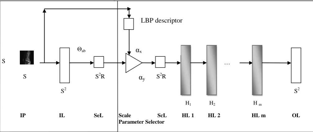
B. TACS-SDANN Architecture
The TACS-SDANN architecture is employed in Figure.1. It contains the sensing and reconstruction layer. Here, the Left-half of the TACS-SDANN architecture [Figure 1] represents the sensing layer (SeL) [linear layer] and the Right-half of the TACS-SDANN architecture [Figure 1] represents the reconstruction layer (non-linear layer). The network takes input as the vectorized image patches (IP) of size n = S2. The n-dimensional input signal x is projecting into the m-dimensional domain in the sensing layer. Thus, the number of units in this layer is m =S2R, where R is the sensing rate, has a value in the range between 0 and 1. The sensing layer has the weights Θab ϵ {-1, 0, +1} m x n, that are corresponding to the projection matrix Θ
ab= ΦT. The first part of the reconstruction layer is a scaling layer. It represents the output of the sensing layer based on the texture feature image linearly by the learned factor α. The scaling layer contains m hidden units. The number of m hidden units of this layer are connected “1-1” and used for compensating the loss which was made by binarizing the sensing weights. The projection matrix is employed in the sensing layer and the learned scaling factor α is kept based on the texture feature image in the reconstruction layer. These layers are followed by m hidden layers. These hidden layers (HL1…m) are using the Rectified Linear Unit (ReLU) activation function [22]. The output layer (OL) is a linear fully connected layer which has a size similar to the input dimension. The HL’s are fully connected in the reconstruction module, followed by a batch-normalization layer that is connected [23].
C. Training Process
Generally, network training uses the standard mini-batch gradient descent method. It is used to obtain the mini patch size of the image. Here, yi, ŷi denotes the input and reconstructed patches, respectively. So yi, ŷi ϵ Rn, n = S2. The mean squared error is obtained between the input and the reconstruction of the image. It is used for obtaining the loss function:
N
L=1 ∑ || yi- ŷi||22 (4) N i=1
Where N is the number of sample image patches. The process of sparsifying and binarization are introduced jointly on the training of the sensing layer opposite to the conventional mini-batch gradient descent method.
In the steps of sparsifying and binarization, the continuous-valued sensing weights Θ ϵ R m x n are sparsified to get the sparse weights Θa ϵ R m x n. In this sparsifying step, the sparse weight Θa contains only the entries that are corresponding to the top-K largest absolute values as Θand set all the remaining entries are to zero. This process is known as a top K-select function. The selection of the top weights in the whole matrix can be assigned column-wise and row-wise. However, since the scaling layer change column-wise operator on the sensing weights, the selection of top K entries can be made column wise. In the sensing layer, each neuron is connected to K = S2 γ elements in the input signal, where γ is the sparsity ratio. A sparse binary mask M ϵ {0, 1} m x n is built with entries that are equal to1 corresponding to the largest weights in Θ implementation wise. The sparse sensing weights are modified according to Θa = M ʘ Θ where ʘ represents the Hadamard product. The process of mapping the sparse continuous-valued weights Θa ϵ R n x m to the sparse binary weights Θ
ab ϵ {-1, 0, +1}m x n is required in binarization. However, both the sparse and binarization step creates some loss that can be recovered during the reconstruction. This layer with weights αx or αy ϵ Rm served as a reverse mapping of the sparse binarized weights Θab to the continuous weights Θ. Thus, the output α Θab
T
y of the scaling layer is obtained by the LBP descriptor adaptive parameter. It is an approximation of ΘTy, corresponding to the continuous projections ΘT. Let θ
(j) and θab(j) be the jth columns of Θ and Θab respectively. θ (j) corresponds to the dense continuous weights of the jth
Figure 1. TACS-SDANN architecture hidden unit in the scaling layer. θ (j) is an approximation of θ
ab(j). The jth entry of the scaling layer weights αx and αy are a scale factor where αx ϵ R+, αy ϵ R+. The values of θab(j) and θ(j) can be obtained by minimizing the following mean square error for θab(j), α(j). Here α(j) is described in the formation of the LBP image.
E= || θ(j)- α(j) θab(j)||22 (5) The equation (5) is expanded as
E= θ(j)T θ(j) - 2 α(j) θ(j)T θab(j) + α(j)2 θ ab(j)T θab(j) (6) Where θ(j)T θ(j) is a constant. As α(j) is a positive scalar [15], and it is taken as an account of the sparsity constraint, the finest sparse binary vector θab(j) obtained as
θab(j)*= argmax(θ(j)T θab(j)) θab(j)
such that θab(j) ϵ {-1,0,+1}m x n
supp (θab(j))=supp(θ a(j)) (7) Where θ a(j) is the jth column of Θa, and supp ʘ denotes the positions of the non-zero entries of the treated vector. The solution of (7) is a vector containing the significations of
θab(j). After obtaining the finest θab(j), the finest θ(j)is solved
by making the derivation of E equal to zero. Considering θ
ab(j)T θab(j) = K, the finest α(j) is given below:
α(j)= 1/K (θ(j)T θab(j))= 1/K (∑i=1n θ(ji) θab(ji) = 1/K (||θ a(j) ||1) (8) At the end of sparsifying and binarization steps, the resultant Θab is sparse and has the K non-zero entries {-1, +1} in each of its columns. After the completion of the existing training algorithms for networks with binary weights [13, 14, 15], the sparse binary weights Θab are used during the forward and backward propagation. The high accuracy weights Θ are used during the update of the parameter Wt, for making the small changes of the weights after the steps of each updating. In the proposed training, Θ is modified using the gradient of loss function for Θab. This process of parameter updating is called an SGD parameter update. It should be marked that Θab contains only discrete weights such as {-1, +1} during the gradient of loss concerning still lies in the continuous domain.
Algorithm
The training of TACS-SDANN is proposed for evaluating the sparse-LBP ternary projection matrix and reconstruction weights at t steps as follows:
Input: Give the patch image x or Y, sparse filter bi; non-linear binarization operator σ; non-linear weight v; Give the weights of continuous and reconstruction domain such as Θ t-1, Wt-1; the learning rate μ.
Procedure for converting the patch image into texture image 1. (xc, yc) = ∑n=0
L=1
s(in, ic) ∙ 2 n
2. s(∙) = 1 if in ≥ ic and s(∙) = 0 otherwise 3. y = ∑i=18 σ(bi * x)∙vi
Procedure for sparsifying and binarizing sensing weights 4. M = top_K_select(Θt-1)
5. Θat= M ʘ Θt-1 6. Θabt = sign(Θat)
7. α jt = 1/K (||θ a(j)||1) for all j ϵ [1,m] Procedure for Forwarding Propagation
8. L= forward(Y, Θabt, Wt-1) Procedure for Backward Propagation
9. (δL/ δ Θabt ), (δL/ δ Wt-1 )=
backward(Y, Θabt, Wt-1) Procedure for Parameter update
10. Wt = update(Wt-1, δL/ δ Wt-1, μ) 11. Θt = update(Θt-1, δL/ δ Θabt, μ)
Output: Find out LBP image y; the loss L; the newly updated weights of continuous and reconstruction domains such as Θt, Wt; the sparse binary sensing weights Θ
abtand the scaling layer weights αjt.
The performance of the proposed TACS-SDANN method is compared with the SDANN method based on the evaluation of mean PSNR using a sparse-LBP ternary projection to check the image quality.
IP IL SeL Scale ScL HL 1 HL 2 HL m OL Parameter Selector
Θab
S2
S S2R
H1 H2 H m
S2 S2R
S …
α
yLBP descriptor
IV. EXPERIMENTAL ANALYSIS
Here, The ILSVRC2012 set [24] is taken for validation, which contains 2000 samples out of 50 K images for training and also the spinal cord dataset is taken for validation, which contains more than 50 K patches for training. These two datasets are taken for comparing with the SDANN and proposed TACS-SDANN model. The proposed model tested on the two testing sets of images with resolution 256x256. The first testing set is taken from the spinal cord dataset and ILSVRC2014 dataset [19] for the comparison between SDANN and the proposed TACS-SDANN algorithm. The second testing set is composed of a randomly selected from the single image in LabelMe dataset [25]. All the images were converted into grayscale in this experiment. It runs in small image patches of size 32 X 32 pixels for reducing the computational overhead. 5 million patches sampled randomly to form the training set. During the training, the input patches of ILSVRC2012 and spinal cord datasets were converted into texture image-based adaptive scale factor. It is processed by subtracting the mean and dividing by the standard deviation. The proposed TACS-SDANN using the proposed training algorithm with the SGD parameter update [26] for a image patch size of 3000, 25 epochs and a learning rate of 0.01 decomposing by a factor of 0.6 every 5 epochs. Also, the SDANN is processed using the proposed training algorithm with the Adam parameter update [26] for the same manner. The training samples were randomly shuffled after each epoch. This out-of-fitting is avoided by the l2 regularization in the
reconstruction layer, with a weight equal to 0.001. During the testing stage, the overlapping patches sampled from each test image with a size of 2 pixels and determined the final image reconstruction as the mean of the patches’ reconstructions. These methods are evaluated using PSNR values. PSNR is expressed in dB. The number of non-linear hidden layer (L) is assigned to 2. Each layer contains 2048 hidden units relating to this network architecture. So this construction produces a good outcome between training time and testing time based on the reconstruction quality. Sensing rate
[image:5.595.307.548.62.139.2] [image:5.595.304.543.473.707.2]The network is trained and tested for different sensing rates by choosing γ = 0.1. The value of R changes in the entries [0.1, 0.3]. The mean PSNR values of the proposed of TACS-SDANN and SDANN method on the first testing set are shown in Table I. The overall reconstruction quality gets better in the larger sensing rates since more information from the signal is retained in a few numbers of measurements as shown in Table I. Hence the proposed TACS-SDANN gives a better reconstruction performance than SDANN.
Table I. Reconstruction Performance for ILSVRC2014 and Spinal Card dataset when varying Sensing rate R
(Choose γ = 0.1) ILSVRC2014
R 0.1 0.15 0.2 0.25 0.3
TACS-SDANN (PSNR dB)
31.66 32.65 33.95 34.69 32.18
SDANN
(PSNR dB) 30.85 30.83 31.22 31.28 31.1
Spinal cord
R 0.1 0.15 0.2 0.25 0.3
TACS-SDANN (PSNR dB)
27.9 28.1 28.36 28.53 28.14
SDANN
(PSNR dB) 22.57 22.6 22.76 22.85 22.74
Sparsity ratio
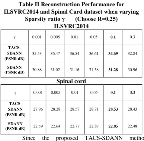
The network is trained and tested with different sparsity ratios γ by choosing R = 0. The mean PSNR values on the first testing set ILSVRC2014 and spinal card are presented in Table II. The result is obtained as Θab∈ {−1, 0, +1}1024×256 for the dimension of input 32 × 32 and R = 0.25. The number of non-zero entries in each column of Θab (i. e. K) are 1, 5, 10, 51, 102, 307 and 1024 respectively. It is represented experimentally as γ ∈ {0.001, 0.005, 0.010, 0.050, 0.100, 0.300, 1.00}. Hence, the finest reconstruction performance can be achieved using extremely sparse projection matrices with only 0.1% non-zero entries (γ = 0.001). The reconstruction performance is improved in the value of γ from 0.001 to 0.05. The network achieves its peak performance in R = 0.25 and produces a slightly worst value for γ ∈ {0.10, 0.30}. It should be noted that there are 256 and 1280 non-zero entries for γ ∈ {0.001, 0.005} in the projection matrix respectively. The previous process is not enough for dealing with the 1024−dimensional input signal. Hence, this is the reason for beginning an obvious performance when γ is increasing from 0.001 to 0.01. During training, the network processes the over-fitting with the reconstructions’ value of γ ∈ {0.1, 0.3}. Hence, γ = 0.05 gives better performance than γ ∈
{0.1, 0.3}. As a result, the proposed sparse binary constraints can be represented as an extra regularizer to the network.
Table II Reconstruction Performance for ILSVRC2014 and Spinal Card dataset when varying
Sparsity ratio γ (Choose R=0.25) ILSVRC2014
γ 0.001 0.005 0.01 0.05 0.1 0.3
TACS-SDANN (PSNR dB)
35.53 36.47 36.54 36.61 34.69 32.84
SDANN
(PSNR dB) 30.88 31.02 31.16 31.38 31.28 30.96
Spinal cord
γ 0.001 0.005 0.01 0.05 0.1 0.3
TACS-SDANN (PSNR dB)
27.96 28.28 28.57 28.71 28.53 28.43
SDANN
(PSNR dB) 22.59 22.64 22.77 22.87 22.85 22.48
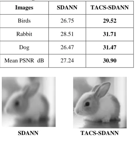
The proposed algorithm uses a non-linear sensing mechanism based on texture feature descriptor, with overlapping image patches of size 32 X 32. The result of ILSVRC2014 and spinal cord datasets on the first testing set are taken. The proposed TACS-SDANN model is trained on the training set for obtaining the results on the second testing set. Sparse binary and ternarius construction like the ones proposed in [27, 28] could not be employed in this experiments due to the constraints impose on matrix dimensions. The comparison of TACS-SDANN with SDANN is obtained using the same sensing rate R = 0.25. Choose γ = 0.05 since it yields the best performance while producing a highly sparse projection matrix. The comparison between the TACS-SDANN and SDANN method on the first testing set of Spinal cord is shown in Table I and II. On the second testing set of LabelMe [25], the mean PSNR values for SDANN and the proposed TACS-SDANN algorithm are 27.24 and 30.90 dB, respectively. Hence, the proposed TACS-SDANN algorithm yields a significantly best result. The proposed TACS-SDANN method provides the sparse ternarius matrix of only 5% of non-zero entries. It is compared to SDANN in terms of recovery performance. Hence, the proposed TACS-SDANN method can provide a better reconstruction quality than the SDANN method using the texture-based adaptive scale.
Table III Reconstruction Performance on different algorithms for Label Me dataset
Images SDANN TACS-SDANN
Birds 26.75 29.52
Rabbit 28.51 31.71
Dog 26.47 31.47
Mean PSNR dB 27.24 30.90
V. CONCLUSION
A TACS-SDANN training algorithm is proposed for the joined mechanism of a highly sparse-LBP ternarius projection matrix and a non-linear reconstruction. It is done for the compressed sensing of the images based on the adaptive scale factor using the LBP descriptor. The TACS-SDANN projection method yields a better reconstruction quality by the value of mean PSNR than the SDANN method. The experimental result shows that the performance of the reconstruction for a projection matrix with 5% non-zero binary entries to be achieved on real images and the corresponding reconstruction trained end-to-end with the proposed TACS-SDANN algorithm. It yields a better result than the SDANN method. The sparse projection
matrices based on texture feature descriptor with only 0.1% non-zero entries are learned using the proposed TACS-SDANN algorithm, that algorithm gives a better performance by the value of mean PSNR than SDANN method.
REFERENCES
1. D. L. Donoho, “Compressed sensing,” IEEE Transaction on Information Theory, vol. 52, no. 4, 2006, pp. 1289–1306.
2. L. Gan, “Block compressed sensing of natural images,” IEEE International Conference on Digital Signal Processing ICDSP, 2007, pp. 403–406.
3. S. S. Chen, D. L. Donoho, and M. A. Saunder , “Atomic decomposition by basis pursuit,” SIAM Journal of Scientific Computing., vol. 20, no. 1, 1999, pp. 33–61.
4. R. Baraniuk, M. Davenport, R. DeVore, and M.Wakin , “A simple proof of the restricted isometry property for random matrices,”
Constructive Approximation, vol. 28, no. 3, 2008, pp. 253–263. 5. C. Dong, C. C. Loy, K. He, and X. Tang, “Image super-resolution
using deep convolutional networks,” IEEE Transaction on Pattern Analysis and Machine Intelligence, vol. 38, no. 2, 2016, pp. 295– 307.
6. P. Vincent, H. Larochelle, I. Lajoie, Y. Bengio, and P. Manzagol, “Stacked Denoising Autoencoders: Learning useful representations in a deep network with a local denoising criterion,” Journal of Machine Learning Research, vol. 11, Dec. 2010, pp. 3371–3408.
7. Mousavi, Ali, Ankit B. Patel, and Richard G. Baraniuk. "A deep
learning approach to structured signal recovery," 53rd Annual
Allerton IEEE Conference on Communication, Control, and Computing (Allerton), 2015.
8. Adler, Amir, et al. "A deep learning approach to block-based
compressed sensing of images," arXiv preprint arXiv: 1606.01519,
2016.
9. M. Elad, “Optimized projections for compressed sensing,” IEEE Transaction on Signal Processing, vol. 55, no. 12, 2007, pp. 5695– 5702.
10. E. Tsiligianni, L. P. Kondi, and A. K. Katsaggelos, “Construction of Incoherent Unit Norm Tight Frames with Application to Compressed Sensing,” IEEE Transaction Information Theory, vol. 60, no.4, 2014, pp. 2319–2330.
11. L. Applebaum, S. D. Howard, S. Searle, and R. Calderbank, “Chirp sensing codes: Deterministic compressed sensing measurements for fast recovery,” Applied Computational and Harmonic Analysis, vol. 26, no. 2, 2009, pp. 283–290.
12. J. D. Haupt, W. U. Bajwa, G. Raz, and R. Nowak, “Toeplitz compressed sensing matrices with applications to sparse channel estimation,” IEEE Transaction on Information Theory, vol. 56, no. 11, 2010, pp.5862–5875.
13. Courbariaux, Matthieu, Yoshua Bengio, and Jean-Pierre David.
"Binaryconnect: Training deep neural networks with binary weights
during propagations." Advances in neural information processing
systems, 2015.
14. Courbariaux, Matthieu, et al. "Binarized neural networks: Training
deep neural networks with weights and activations constrained to +1
or -1," arXiv preprint arXiv: 1602.02830, 2016.
15. Rastegari, Mohammad, et al. "Xnor-net: Imagenet classification
using binary convolutional neural networks," European Conference
on Computer Vision. Springer, Cham, 2016, pp. 525-542.
16. S.Han, J.Pool, J.Tran, & W.Dally, “Learning both weights and
connections for efficient neural network,” Advances in neural
information processing systems, 2015, pp. 1135-1143.
17. S. Han , H. Mao, and W. J. Dally, “Deep compression – compressing deep neural networks with pruning, trained quantization, and Huffman coding,” in International Conference on Learning Representations (ICLR), 2016.
18. F. Juefei-Xu , K. Luu, and M. Savvides. Spartans: Singlesample Periocular-based Alignment-robust Recognition Technique Applied to Non-frontal Scenarios. IEEE Transaction on Image Processing, Dec 2015, 24(12):4780–4795.
19. F. Juefei-Xu and M. Savvides. Subspace-Based Discrete Transform Encoded Local Binary Patterns Representations for Robust Periocular Matching on NIST’s Face Recognition Grand Challenge.
IEEE Transaction on Image Processing, Aug 2014, 23(8):3490– 3505.
20. F. Juefei-Xu and M. Savvides., Learning to Invert Local Binary Patterns. In 27th British Machine Vision Conference BMVC, Sept 2016.
21. [21] Y. LeCun, L. Bottou, Y. Bengio, and P. Haffner. Gradient-based Learning Applied to Document Recognition. Proceedings of the IEEE, 1998, 86(11):2278–2324.
22. X. Glorot, A. Bordes, and Y. Bengio, “Deep sparse rectifier neural networks,” in Proceedings of the fourteenth International Conference on Artificial Intelligence and Statistics (AISTATS), 2011, pp. 315–323.
23. S. Ioffe and C. Szegedy, “Batch normalization: Accelerating deep network training by reducing internal covariate shift,” International Conference on Machine Learning (ICML), 2015, pp. 448–456. 24. O. Russakovsky, J. Deng, H. Su, J. Krause, S. Satheesh, S. Ma, Z.
Huang, A. Karpathy, A. Khosla, M. Bernstein, A. C. Berg, and L. Fei-Fei, “Imagenet large scale visual recognition challenge,”
International Journal of Computational Vision, vol. 115, no. 3, 2015, pp. 211–252.
25. B. C. Russell, A. Torralba, K. P. Murphy, and W. T. Freeman, “Labelme: A database and web-based tool for image annotation,”
International Journal of Computational Vision, vol. 77, no. 1-3, 2008, pp. 157173.
26. D. P. Kingma and J. L. Ba, “Adam: A method for stochastic optimization,” in International Conference on Learning Representations (ICLR), 2015.
27. S.Li and G. Ge, “Deterministic construction of sparse sensing matrices via finite geometry,” IEEE Transaction on Signal Processing, vol. 62, no. 11, 2014, pp. 2850–2859.
28. A. Amini and F. Marvasti, “Deterministic construction of Binary, Bipolar and Ternary compressed sensing matrices,” IEEE Transaction on Information Theory, vol. 57, no. 4, 2011, pp. 2360– 2370.
AUTHORS PROFILE
D.M.Annie Brighty Christilin is working as Assistant Professor, Department of Computer Science, Sadakathullah Appa College, Tirunelveli. She has completed M.C.A., M.Phil in Manonmaniam Sundarnar University and also SET. She is involved in various academic activities. She has presented international and national conference papers. She is a member of google scholar. She is a member of various committees in autonomous college and She is a Research Scholar of Computer Science in Manonmaniam Sunadaranar University under the guidance of the Second author.