Development of Regional Flood Frequency Relationship for Narmada Basin using Index Flood Procedure

(1)

International Journal of Innovative Technology and Exploring Engineering (IJITEE) ISSN: 2278-3075, Volume-8 Issue-12, October 2019



Abstract: Water Resources decision making problems such as flood plain zoning, design of hydraulic structures etc. are based on design flood estimate, defined as discharge for a specified probability of exceedance. Flood Frequency Analysis helps to estimate the flood value for a specific return period. This procedure requires sufficient length of observed data of floods on river gauging sites which many a time is not available. In India major rivers have very few gauging sites and their tributaries are mostly ungauged. When quantiles have to be estimated for ungauged sites, Flood Frequency Analysis is neither possible nor reliable. Regional Flood Frequency Analysis is the means to overcome such problems, reasonably quantifying flood estimates at desired frequencies for sites within a more or less hydrological homogeneous region. Narmada Basin located in central India covers an area about 98,976 sq. km, drained by a large number of tributaries, most of which are ungauged, has been considered as the case. Index Flood method utilizing Gumbel’s EV-1 distribution have been used in the present study to develop the Regional flood frequency relationship. The Annual Peak Flood data of 16 gauging sites of Narmada Basin, having record length of 12 to 17 years, is utilized for flood estimation. Flood frequency curves for the considered gauging stations are generated. Development of regional flood frequency relationship leads to the estimation of different return period flood.

Index Terms: Gumbel’s EV-1 distribution, Index flood method, Regional flood frequency relationship, Return period flood.

I. INTRODUCTION

Planning and construction of large number of hydraulic structures is required at all possible locations in different river basins to achieve the sustainable development of the country and to meet the ever-increasing demand of water. While designing the project, major constraint experienced by the project planner is to decide the value of worst flood (design flood) which the hydraulic structure may experience during its lifetime. On the basis of the design flood, hydraulic design and construction of the structure such as Dams, Barrages, Diversion structures etc. is possible. Faulty estimation of the design flood can cause the failure of the structure due to heavy flood flow. The problem of floods and their computation is one of the main and most complex problems faced by the hydrologists. Design of various hydraulic structures such as, Spillways, Barrages, and Levees etc. requires a realistic estimation of floods of various return periods. Realistic flood estimation is also needed for the use of non-structural means for reducing the flood damage. The flood frequency analysis procedures based on statistical and probability concept are usually employed to determine the

flood value for a given return period. The flood data from the stream gauging sites is required for the analysis which has to satisfy the criteria of homogeneity, independence, randomness and time invariance. However, the procedures are not suitable for those catchments which are either ungauged or have a very scanty data for gauging. Further, there is a rising trend for constructing small projects in place of large projects due to their relative merits such as, early completion, small investment and early return of investment. These small projects are usually constructed on small watersheds, which are normally ungauged or have very little data of annual flood discharge. This requirement has necessitated the development of rational methodologies for evolving Design Floods for such small catchments.

when the data available is limited or when there is no record available at site, the “Regional Flood Frequency Approach” provides reasonable estimates of expected floods In order to have consistent approach for a region, it is necessary to develop standard procedures and guidelines for deciding about homogeneity of the region, choice of distributions, methods of parameter estimation and relationship of peak flood characteristics with catchment characteristics. This is the typical case in Narmada Basin, where most of its tributaries are ungauged.

II. STUDYAREA

The Narmada Basin located in central India has been selected as the study area in present study. The Narmada Basin covers an area of 98796 sq. km and is located between longitudes 72032'E to 810 45' E and latitudes 21020' N to 23045'N. The major part of the basin lies in Madhya Pradesh State while a small part of it lies in the states of Maharashtra and Gujrat. The Basin is bounded on north by Vindhyas, on th east by the Maikala Range, on the south by Satpura and on the west by Arabian Sea. The Narmada River is the largest river in India flowing east to west. It rises in the Amarkantak Plateau of Maikala range in the Shahdol district of Madhya Pradesh at an elevation of 1057 meters above mean sea level at a latitude 22040' north and a longitude of 81045' east. The river travels a distance of 1,312 km before it falls into Gulf of Cambay in the Arabian Sea near Bharuch in Gujarat. The first 1,079 km of its run are in Madhya Pradesh and Maharashtra. The last length of 159 km lies in Gujarat.

Development of Regional Flood Frequency

Relationship for Narmada Basin using Index

Flood Procedure

(2)

The river has 41 tributaries in all, each having catchment area of more than 500 sq.kms out of these 41 tributaries 22 are on Southern bank and 19 on the Northern side. 39 tributaries are situated in M.P. and 2 are in Gujarat. Among all tributaries the “Hiran” is the longest having length of 188 kms. and the Tawa has largest catchment area 6067 sq.kms. The major left side tributaries are Burhner, Banjar, Hiran, Sher, Shakkar, Dudhi, Tawa, Ganjal, ChhotaTawa, Kundi, Goi. The major right-side tributaries are Hiran, Tedoni, Barna, Kolar, Maan, Uri, Hatni, Orsang. The temperature of the basin touches a maximum of 480C in the month of May while minimum of 1.70C is recorded in the month of December. The average relative humidity value is very low in dry weather being 12% and is maximum in the monsoon season with value of 87.5%. The estimated average Rainfall of the basin is 1245mm. The monsoon rainfall from June to September is 92% of the annual rainfall.

III. DATAACQUISITION

The annual peak flood series data set varying from 12 to 17 years for 16 gauging sites of Narmada Basin have been utilized in the present study. The range of annual peak flood, length of data records available and catchment area for various catchments are summarized in Table-I.

Table-I: Data of peak flood of gauging stations S.

No.

Gauging

Station Area km 2 Record Length Years Annual Peak flood Cumec

1 Mannot 4300 12 960-6180

2 Jamtara 17157 17 2299-2135

3 Barmanghat 26458 17 1992-20658

4 Sandia 33953 12 3850-16500

5 Hoshangabad 44548 16 5853-3359

6 Handia 54027 12 3600-26240

7 Mandleshwar 72809 17 9979-46000

8 Mohgaon 4661 12 691-9000

9 Hriday Nagar 3770 12 502-2492

10 Belkheri 1508 12 84-6500

11 Gadarwara 2270 12 724-3030

12 Rajghat 77674 17 9600-56610

13 Garudeshwar 87892 17 7707-49500

14 Bagratawa 6018 12 299-25574

15 Chhidgaon 1729 12 197-4470

16 Ginnore 4815 17 1026-12157

IV. METHODOLOGY

For the evaluation of flood magnitudes of different return periods in ungauged watersheds of Narmada Basin the Index Flood method of Regional Flood Frequency Analysis has been adopted in the present study. Index Flood method utilizes the data of the gauged catchments to evaluate a regional relationship from which the flood magnitudes of various return periods for ungauged catchments can be evaluated.

A. Selection of Gauged Catchments

The first step is to identify those gauged catchments whose data can be used. These gauged catchments should have the similar physiographic, hydrologic and Metrologic characteristics as exists in ungauged catchments. Annual peak flood data of all the sixteen gauging stations have been found suitable.

B. Data Requirement

The major data which is required for the analysis with the Index Flood Method is the observed annual peak flood. The data collected have been observed at the gauging sites under unregulated and consistent site conditions.

C. Base Period Determination

Before the homogeneity of the data can be tested, a time base period, the longest period of record during which data from each gauging site is utilized for analysis is established. In the present study a base period of 10 years i.e. data of only those sites have been considered for the analysis which were having records more than or equal to 10 years.

D. Flood Frequency Curves

After establishing the length of record that is to be used at each and every station, the annual maximum flood series is ranked and the corresponding plotting position for each flood value has been calculated using Gringorton Plotting Position Formula.

Pi = (i – 0.44 ) / ( N + 0.12 ) (1)

Where, Pi is the Probability of Non- exceedance of an event, i is the rank of the event, and N is the number of years of record.

Using the ranked annual maximum flood series and the corresponding plotting positions, the frequency curves have been developed by plotting the peak discharge value against the values of Gumbel’s EV-1 reduced variate on an ordinary graph paper for each gauging site. Following equation has been used to calculate the reduced variate (yi) for Gumbel’s EV-1 distribution for any peak discharge value.

yi = - ln [- ln (Pi) ] (2)

Where, yi is EV-1 reduced variate corresponding to plotting position Pi.

(3)

The suitability of the straight line fitted for the observations on graph paper as mentioned above, is required to be checked as envisaged by Dalrymple (1960). The check has been performed in the study by constructing 95% confidence interval using the upper and lower confidence intervals as given by Hann (1977).

The flood frequency curves have been developed for all the 16 gauging stations following the above-mentioned procedure and the straight lines of the following form have been fitted:

QT = a + b YT (3)

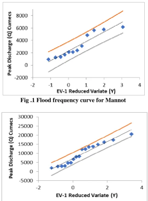
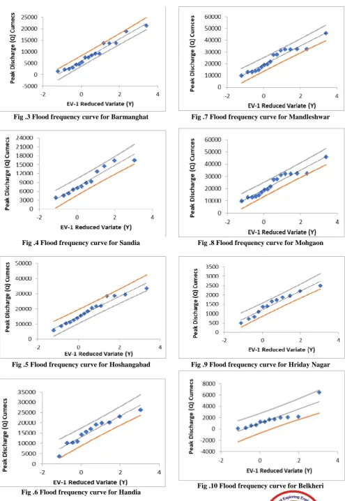
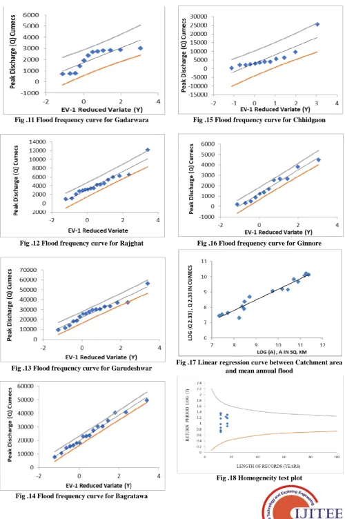
Where, YT is the reduced variate, QT is flood magnitude for return period of T years, and a, b, are the constants. The developed flood frequency curves along with the confidence limits are shown in Fig. 1 to Fig. 16. The derived equations of flood frequency curves are given in Table-II.

E. Mean Annual Flood

The Mean Annual Flood flow magnitude corresponding to an average return period of 2.33 years. It is denoted by Q2.33.

F. Homogeneity Test

The homogeneity of the runoff data from the gauged catchments is measured with respect to the static defined by the ratio of 10-year flood to the mean annual flood (Q2.33). The 10-year flood which is equivalent to the flood magnitude having a probability of non-exceedance of 90%. In the present study the data of selected 16 gauged catchments have been checked for homogeneity by applying the test. It is found that the data at all the 16 stations have passed the homogeneity test. The computations for Homogeneity Curve are shown in Table-III & IV and the Homogeneity Test Plot is shown in Fig. 18.

G. Relationship of Mean Annual Flood and Catchment Area

After performing the homogeneity test, a relationship of the following type is developed as the further part of analysis.

Q2.33 = CAn (4)

Where, Q2.33 is the mean annual flood value, A is the catchment area, and C and n are the region constants. For the present study the regression analysis has been carried out using the data of all the 16 gauging sites and the values of constants C and n have been derived as 9.79 and 0.689 respectively with a value of r2 = 0.943. The developed equation will provide the value of mean annual flood for any ungauged catchment knowing its area only. The plot of log (Q2.33) and log (A) indicating the developed relationship is shown in Fig. 17.

H. Regional Flood Frequency Relationship

The final step is to develop the regional flood frequency relationship for determining the values of flood for different return periods for ungauged catchments. The entire computation is shown in Table-V. The developed regional

QT / Ǭ = a + b YT (5)

Where, QT is T year flood, Ǭ is the mean annual flood (Q2.33), YT is the EV-1 reduced variate, a and b are constants.

I. Estimation of T-Year Flood for an Ungauged Catchment

Using the relationship developed in the previous steps under Index Flood method, The T-Year flood value for an ungauged catchment of river Narmada can be determined. In the present study 20, 50, 100, 500 and 1000-year flood values at each gauged discharge site of the study area have been obtained and shown in Table-VI.

V. RESULTSANDDISCUSSION A. Flood Frequency Curves

[image:3.595.306.550.356.688.2]

It is found that all the points for each gauging site falls under these confidence limits. The derived curves are shown in Fig. 1 to Fig. 16. The equation for each curve has also been developed using technique of linear regression. The developed equation for all the 16 gauging sites is given in Table-II along with the r2 values. The value of r2 varies from 0.737 to 0.983 which shows the strong validity of the fitted straight lines of frequency curves.

Fig .1 Flood frequency curve for Mannot

(4)

Fig .3 Flood frequency curve for Barmanghat

Fig .4 Flood frequency curve for Sandia

[image:4.595.52.548.43.762.2]

Fig .5 Flood frequency curve for Hoshangabad

Fig .6 Flood frequency curve for Handia

Fig .7 Flood frequency curve for Mandleshwar

Fig .8 Flood frequency curve for Mohgaon

Fig .9 Flood frequency curve for Hriday Nagar

(5)

Fig .11 Flood frequency curve for Gadarwara

Fig .12 Flood frequency curve for Rajghat

[image:5.595.50.551.44.797.2]

Fig .13 Flood frequency curve for Garudeshwar

Fig .14 Flood frequency curve for Bagratawa

Fig .15 Flood frequency curve for Chhidgaon

Fig .16 Flood frequency curve for Ginnore

Fig .17 Linear regression curve between Catchment area and mean annual flood

(6)

Table-II: Equation of Frequency Curves for Different Catchments

Sl.No. Station Equation of Frequency Curve Correlation Coefficient (R) R2

1 Mannot QT = 2277.815 + 1542.502 YT 0.947629 0.898

2 Jamtara QT = 5982.647 + 4781.954 YT 0.984886 0.97

3 Barmanghat QT = 7120.207 + 4663.931 YT 0.969536 0.94

4 Sandia QT = 7462.734 + 3641.194 YT 0.966437 0.934

5 Hoshangabad QT = 14916 + 6678.652 YT 0.978264 0.957

6 Handia QT = 13099 + 5119.814 YT 0.960208 0.922

7 Mandleshwar QT = 19394 + 7892.705 YT 0.966437 0.934

8 Mohgaon QT = 1581.26 + 1967.48 YT 0.94921 0.901

9 Hriday Nagar QT = 1211.208 + 499.8169 YT 0.972111 0.945

10 Belkheri QT = 990.6154 + 1268.795 YT 0.903881 0.817

11 Gadarwara QT = 1718.33 + 664.10 YT 0.858487 0.737

12 Rajghat QT = 22143 + 9141.911 YT 0.973653 0.948

13 Garudeshwar QT = 19741.35 + 9433.789 YT 0.991464 0.983

14 Bagratawa QT = 3080.749 + 4892.8848 YT 0.875214 0.766

15 Chhidgaon QT = 1242.949 + 1138.327 YT 0.984378 0.969

16 Ginnore QT = 3121.887 + 2062.20 YT 0.961769 0.925

Table -III: Computation of Frequency Ratio

S.No. Station Equation of Regression Line Q2.33 Q10 Q10 / Q2.33 = α

1 Mannot QT = 2277.815 + 1542.502 YT 3169.381 5748.444 1.813743

2 Jamtara QT = 5982.647 + 4781.954 YT 8746.385 16741.14 1.914064

3 Barmanghat QT = 7120.207 + 4663.931 YT 9815.959 17614.05 1.79443

4 Sandia QT = 7462.734 + 3641.194 YT 9567.344 15655.42 1.636339

5 Hoshangabad QT = 14916.00 + 6678.652 YT 18776.26 29942.97 1.594725

6 Handia QT = 13099.00 + 5119.814 YT 16058.25 24618.58 1.53308

7 Mandleshwar QT = 19394.00 + 7892.705 YT 23955.98 37152.59 1.550869

8 Mohgaon QT = 1581.26.00 + 1967.48 YT 2718.46 6008.9 2.210406

9 Hriday nagar QT = 1211.208 + 499.8169 YT 1500.102 2335.796 1.557091

10 Belkheri QT = 990.6154 + 1268.795 YT 1723.978 3845.404 2.230541

11 Gadarwara QT = 1718.33.00 + 664.10 YT 2102.179 3212.555 1.528202

12 Rajghat QT = 22143.00 + 9141.911 YT 27427.02 42712.3 1.557307

13 Garudeshwar QT = 19741.35 + 9433.789 YT 25194.08 40967.37 1.626071

14 Bagratawa QT = 3080.74 + 4892.8848 YT 5908.836 14089.74 2.38452

15 Chhidgaon QT = 1242.949 + 1138.327 YT 1900.902 3804.184 2.001252

16 Ginnore QT = 3121.887 + 2062.20 YT 4313.838 7761.837 1.799288

_{Mean α =}

1.7957 Table-IV:Homogeneity Test Computation Details

Sl.No. Station Qt = ᾱ Q 2.33 Equation for Computation of Yt Yt

T (Years)

Length of Records

1 Mannot 5691.257462 YT = (QT - 2277.815) / 1542.505 2.21 9.62 12

2 Jamtara 15705.88354 YT = (QT - 5982.647) / 4781.554 2.033 8.14 17

3 Barmanghat 17626.51776 YT = (QT - 7120.207) / 4663.931 2.25 9.99 17

4 Sandia 17180.07962 YT = (QT - 7462.734) / 3641.194 2.66 14.92 12

5 Hoshangabad 33716.53008 YT = (QT - 14916) / 6678.652 2.81 17.19 16

6 Handia 28835.80312 YT = (QT - 13099) / 5119.814 3.073 22.12 12

(7)

Table-V: Computation Detail for Regional Flood Frequency Relationship

Sl. No. Station Q2.33 Q10 Q50 Q100 Q500 Q1000

1 Mannot 11856.750 12921.070 35678.580 38978.120 36083.210 39301.330

2 Jamtara 30074.540 32586.970 56390.420 60998.690 44893.040 48425.710

3 Barmanghat 68407.690 73853.665 13799.310 15156.870 4315.070 4659.944

4 Sandia 8869.830 9745.300 5842.390 6300.620 78914.260 85222.180

5 Hoshangabad 78325.170 84834.490 33465.560 36841.650 8311.950 9097.400

6 Handia 15928.140 17351.060 5748.444 16741.144 17614.051 15655.421

7 Mandleshwar 29942.967 24618.581 37152.586 6008.900 2335.796 3845.404

8 Mohgaon 3212.555 42712.299 40967.370 14089.740 3804.184 7761.837

9 Hriday Nagar 8293.570 24632.260 25309.530 21663.390 40962.740 33066.270

10 Belkheri 50175.540 9254.430 3160.490 5938.910 4308.320 57796.450

11 Gadarwara 56533.120 22162.990 5682.420 11164.460 9373.310 27979.630

12 Rajghat 28574.280 24212.220 45637.790 36650.144 55700.443 10631.660

13 Garudeshwar 3510.360 6827.070 4773.190 64195.790 63136.770 25588.010

14 Bagratawa 6479.250 12608.007 3169.381 8746.385 9815.959 9567.344

15 Chhidgaon 18776.260 16058.252 23955.980 2718.460 1500.102 1723.978

16 Ginnore 2102.179 27427.024 25194.080 5908.836 1900.902 4313.838

Table-V (cont.): Computation Detail for Regional Flood Frequency Relationship Sl. No. Station Q10/Q2.33 Q50/Q2.33 Q100/Q2.33 Q500/Q2.33 Q1000/Q2.33

1 Mannot 3.741 4.077 4.079 4.456 3.676

2 Jamtara 4.004 3.143 3.406 3.003 3.249

3 Barmanghat 2.796 3.016 2.856 3.083 5.076

4 Sandia 5.576 2.877 3.106 5.145 5.653

8 Mohgaon 4881.538622 YT = (QT - 1581.26) / 1967.48 1.67 5.86 12

9 Hriday Nagar 2693.733161 YT = (QT - 1211.208) / 499.8169 2.96 19.92 12

10 Belkheri 3095.747295 YT = (QT - 990.6154) / 1268.795 1.65 5.77 12

11 Gadarwara 3774.88283 YT = (QT - 1718.330) / 664.10 3.09 22.62 12

12 Rajghat 49250.707 YT = (QT - 22143) / 9141.911 2.96 19.9 17

13 Garudeshwar 45241.00946 YT = (QT - 19741.35) / 9433.189 2.7 15.43 17

14 Bagratawa 10610.49681 YT = (QT - 3080.749) / 4892.8848 1.53 5.17 12

15 Chhidgaon 3413.449721 YT = (QT - 1242.99) / 1138.327 1.906 7.24 12

(8)

5 Hoshangabad 2.779 2.997 2.877 3.107 3.109

6 Handia 3.367 5.664 6.235 4.373 4.786

7 Mandleshwar 3.692 4.022 2.617 2.816 2.578

8 Mohgaon 2.264 2.182 2.059 2.094 3.404

9 Hriday Nagar 2.107 3.445 2.049 2.107 2.244

10 Belkheri 3.751 2.989 2.588 2.957 3.199

11 Gadarwara 2.911 2.531 2.431 2.282 2.325

12 Rajghat 3.911 2.34 3.96 2.271 2.341

13 Garudeshwar 2.506 4.33 3.409 2.923 1.814

14 Bagratawa 1.914 1.794 1.636 1.595 1.533

15 Chhidgaon 1.551 2.21 1.557 2.231 1.528

16 Ginnore 1.557 1.626 2.385 2.001 1.799

Median 3.707 2.422 2.72 3.409 1.715

Table-VI: Return Period Floods By Index Flood Method

Sl.No Station

Index Flood

Q20 Q50 Q100 Q500 Q1000

1 Mannot 6310.416 7552.552 8487.493 10637.86 11559.44

2 Jamtara 16373 19595.85 22021.64 27600.98 29992.12

3 Barmanghat 22066.83 26410.45 29679.83 37199.42 40422.1

4 Sandia 26204.61 31362.7 35245.13 44174.73 48001.7

5 Hoshangabad 31596.64 37816.09 42497.39 53264.4 57878.83

6 Handia 36088.35 43191.95 48538.74 60836.37 66106.78

7 Mandleshwar 44324.61 53049.43 59616.49 74720.74 81193.99

8 Mohgaon 6670.837 7983.918 8972.258 11245.44 12219.66

9 Hriday Nagar 5763.647 6898.158 7752.091 9716.136 10557.87

10 Belkheri 3065.609 3669.04 4123.236 5167.886 5615.593

11 Gadarwara 4063.498 4863.353 5465.394 6850.089 7443.53

12 Rajghat 46344.54 55466.95 62333.28 78125.84 84894.09

13 Garudeshwar 50463.73 60396.96 67873.58 85069.82 92439.63

14 Bagratawa 7955.011 9520.867 10699.47 13410.25 14572.02

15 Chhidgaon 3368.519 4031.575 4530.649 5678.52 6170.465

16 Ginnore 6822.61 8165.566 9176.393 11501.3 12497.68

B. Mean Annual Flood – Catchment Area Relationship The relationship between mean annual flood and catchment area has been developed using the regression technique and utilizing the data of 16 gauging sites in Narmada Basin. Following relationship has been derived:

Q2.33 = 9.79 A 0.689 (6)

The r2 value of the above relationship is 0.943 which shows a strong correlation between the parameters Q2.33 and A and also the validity of equation. The plot showing the relationship between Q2.33 and A is shown in Fig. 17.

C. Regional Flood Frequency Relationship

For estimating the value of flood for a return period in any ungauged catchment of Narmada Basin a regional flood

frequency relationship has been developed based on Gumbel EV – 1 distribution. The developed relationship is as follows:

QT / Ǭ = 0.751 + 0.428 YT (7)

The r2 value for the above developed curve has been obtained as 1.0 which shows the strongest correlation and its validity.

VI. CONCLUSION

(9)

• The relationship between mean annual flood and

catchment area using regression analysis, has been derived as Q2.33 = 9.79 A 0.689

• The Gumbel’s Extreme Value Type I distribution more closely fits the annual flood data at most of the gauging sites of Narmada Basin.

• All the considered 16 gauging sites of Narmada Basin are hydrologically homogenous and falls under homogeneity criteria.

REFERENCES

1. Burn,D.H., and Goel,N.K. (2000). “The Formation of Groups for Regional Flood Frequency Analysis”. Hydrological Sciences Journal, Vol.45, No.1, pp. 97-112.

2. Cannarozzo,M., Dasaro,F., and Ferro,V. (1995). “Regional Rainfall and Flood Frequency Analysis for Sicily using the Two Component Extreme value distribution”. Hydrological Sciences Journal, Vol.40, No.1, pp. 19-42.

3. Chavoshi,S., and Soleiman,W.N.A. (2009). “Delinating Pooling Group for Flood Frequency Analysis Using Soft Computing”. European Journal of Scientific Research, Vol.35, No.2, pp. 181-187.

4. Fiorentino,M., Gabriele,S., Rossi,F., and Versace,P. (1987). “Hierarchical Approach for Regional Flood Frequency Analysis”. V.P.Singh (eds), Regional Flood Frequencu Analysis, D.Reidel Publishing C ompany, pp. 35-49.

5. Gaume,E., Gaal,L., Viglione,A., Szolgay,J., Kohnova,S., and Bloschl,G. (2010). “Bayesian MCMC Approach to Regional Flood Frequency Analysis involving Extraordinary Flood Events at Ungauged Sites”. Journal of Hydrology, 2010 Elsevier science, pp. 1-17.

6. Hassan,G.H., and Ping,F. (2011). “Regional Flood Frequency Analysis-Launhe basin-Hebei-China”. Interternational Conference on Humanities, Geography and Economics (ICHGE 2011), Pataya, pp. 316-328.

7. Heo,J.H., Boes,D.C., and Salas,J.D. (2001). “Regional Flood Frequency Analysis based on Weibull model: Part 1. Estimation and Asymptotic Variances”. Journal of Hydrology, Vol.242, Elsievier science, pp. 157-170.

8. Heo,J.H., Salas,J.D., and Boes,D.C. (2001). “Regional Flood Frequency Analysis based on Weibull model: Part 2. Simulation and applications”. Journal of Hydrology, Vol.242, Elsevier science, pp. 171-182.

9. Hosking, J.R. and Wallis, J.R. (1993). “Some statistics useful in regional frequency analysis”. Water Resour. Res., Vol. 29(2), pp. 271-281

10. Kao,S.C., and Chang,N.B. (2012). “Copula Based Flood Frequency Analysis at Ungauged Basin Confluences: Nashville, Tennessee”. Journal of Hydrologic Engineering,Vol.17, No.7, ASCE, pp. 790-799. 11. Kar,A.K., Goel,N.K., Lohani,A.K., and Roy,G.P. (2012). “Application of Clustering Technique using Priotised Variables in Regional Flood Frequency Analysis: Case study of Mahanadi Basin”. Journal of Hydrologic Engineering, Vol.17, No.1, ASCE, pp. 213-223. 12. Koulouris,A.Z.,Vogel,R.M., Craig,S.M., and Habermeier,J. (1998). “L

moments diagrams for censored observation”.Water Resources Research, Vol.34, No.5, American Geophysical Union, pp. 1241-1249. 13. Lim,Y.H., and Voeller,D.L. (2009). “Regional Flood Estimation in Red River Using L-Moment Based Index Flood and Bulletin 17B Procedures”. Journal of Hydrological Engineering, Vol.14, No.9, ASCE, pp. 1002-1016.

14. National Institute of Hydrology (1997-1998). A Report on “Regional Flood Frequency Analysis using L-Moments”. Roorkee.

15. National Institute of Hydrology (2000-2001). A Report on “Develpoment of Regional Flood Formulate using L-Momemts for Middle Ganga Plains (Subzone 1-F)”.Roorkee.

16. Saf,B.(2008). “Regional Flood Frequency Analysis Using L-Moments for the West Mediterranean Region of Turkey”. Water Resource Manage, Vol.23, pp. 531-551.

17. Shi,P., Chen,X., Qu,S.M., Zhang,Z.C., and Ma,J.L. (2010). “Regional Frequency Analysis of Low Flow based on L-Moments: Case study in Karst Area, SouthWest China”. Journal of Hydrological Engineering, Vol.15, No.5, ASCE, pp. 370-377.

18. Smith,J.A. (1989). “Regional Flood Frequency Analysis Using Extreme Order Statistics of Annual Peak Record”. Water Resources Research, Vol.25, No.2, pp. 311-317.

19. Sveinsson,G.B., Boes,D.C., and Salas,J.D. (2001). “Population Index Flood Method for Regional Frequency Analysis”. Water Resources Research, Vol.37, No.11, pp. 2733-2748.

20. Thorvat,A.R., and Mujumdar,M.M. (2011). “Design Flood Estimation for Upper Krishna Basin through RFFA”. International Journal of Engineering Science and Technology (IJEST), Vol.3, No.6, pp. 5252-5259.

AUTHORSPROFILE