The effect of railway local irregularities on ground vibration

This is a repository copy of

The effect of railway local irregularities on ground vibration

.

White Rose Research Online URL for this paper:

http://eprints.whiterose.ac.uk/125156/

Version: Accepted Version

Article:

Kouroussis, G, Connolly, DP, Alexandrou, G et al. (1 more author) (2015) The effect of

railway local irregularities on ground vibration. Transportation Research Part D: Transport

and Environment, 39. pp. 17-30. ISSN 1361-9209

https://doi.org/10.1016/j.trd.2015.06.001

© 2015, Elsevier Ltd. Licensed under the Creative Commons Attribution

NonCommercial-NoDerivatives 4.0 International

http://creativecommons.org/licenses/by-nc-nd/4.0/

[email protected] Reuse

This article is distributed under the terms of the Creative Commons Attribution-NonCommercial-NoDerivs (CC BY-NC-ND) licence. This licence only allows you to download this work and share it with others as long as you credit the authors, but you can’t change the article in any way or use it commercially. More

information and the full terms of the licence here: https://creativecommons.org/licenses/

Takedown

If you consider content in White Rose Research Online to be in breach of UK law, please notify us by

Georges Kouroussis1_{, David P. Connolly}2_{, Georgios Alexandrou}1_{, and Konstantinos Vogiatzis}3

1University of Mons — UMONS, Faculty of Engineering, Department of Theoretical Mechanics, Dynamics and Vibrations, Place du Parc 20, B-7000 Mons, Belgium

2Heriot-Watt University, School of Energy, Geoscience, Infrastructure & Society, Edinburgh EH14 4AS, United Kingdom

3University of Thessaly, School of the Civil Engineering, Pedion Areos, 383 34 Volos, Greece

Abstract

The environmental effects of ground-borne vibrations generated due to localised railway defects is a growing concern in urban areas. Frequency domain modelling approaches are well suited for predicting vibration levels on standard railway lines due to track periodicity. However, when considering individual, non-periodic, localised defects (e.g. a rail joint), frequency domain modelling becomes challenging. Therefore in this study, a previously validated, time domain, three-dimensional ground vibration prediction model is modified to analyse such defects. A range of different local (discontinuous) rail and wheel irregularity are mathematically modelled, including: rail joints, switches, crossings and wheel flats. Each is investigated using a sensitivity analysis, where defect size and vehicle speed is varied. To quantify the effect on railroad ground-borne vibration levels, a variety of exposure-response relationships are analysed, including: peak particle velocity, maximum weighted time-averaged velocity and weighted decibel velocity. It is shown that local irregularities cause a significant increase in vibration in comparison to a smooth track, and that the vibrations can propagate to greater distances from the line. Furthermore, the results show that step-down joints generate the highest levels of vibration, whereas wheel flats generate much lower levels. It is also found that defect size influences vibration levels, and larger defects cause greater vibration. Lastly, it is shown that for different defect types, train speed effects are complex, and may cause either an increase or decrease in vibration levels.

Keywords:

wheel/rail impact; vehicle/track interaction; railroad ground-borne vibration; environmental impact assessment; flat wheel; local track irregularities

1. Introduction

Railway induced ground vibrations can cause negative effects on urban environments situated near

rail lines. The propagation of railway vibrations (particularly in urban areas) is complex, due to

the different transmission paths within a medium that is fundamentally inhomogeneous, non-engineered and infinite in three directions. There is a large body of research into railway-induced ground vibra-tions, such as their effect on urban environments and potential mitigation measures (e.g. wave imped-ing blocks (Coulier et al., 2013), trenches (Connolly, Giannopoulos, Fan, Woodward and Forde, 2013) or

wave barrier (Garinei et al., 2014)). Furthermore, for high-speed trains (Degrande and Schillemans, 2001; Galvín and Domínguez, 2009; Costa et al., 2010; Connolly et al., 2015), research is currently motivated by the so-called “supercritical phenomenon” which occurs when the vehicle speed is close to the Rayleigh

ground wave speed. Critical speed depends on the soil flexibility and may be close to that of

con-ventional high-speed lines (Madshus and Kaynia, 2000; Connolly, Kouroussis, Laghrouche, Ho and Forde,

2014). Despite the large vibration levels generated by these lines which are underlain by soft

soils (Connolly, Kouroussis, Woodward, Costa, Verlinden and Forde, 2014), the distance d between the

track and neighbouring structures is relatively high and the vibration attenuates rapidly. In

the case of railway traffic, the attenuation is associated with a power law of the form d−q,

where q lies between 0.5 and 1.1, depending on the soil configuration (Auersch and Said, 2010).

Connolly, Kouroussis, Woodward, Verlinden, Giannopoulos and Forde (2014) proposed that it is possible to establish relationships between six key railway variables for ground vibration metrics in the case of high-speed lines. The situation is significantly different for the case of urban transit, because:

• The distancedbetween track and building is relatively close.

• The contribution of the vehicle weight and speed (quasi-static effects) is low.

• The presence of local defects induces elevated localised vibrations (dynamic effects).

Local defects are a significant source of dynamic excitation on railway tracks. Accurate descriptions of the interaction between the track and the vehicle have been modelled by Nielsen and Abrahamsson (1992), Zhai and Sun (1994); Zhai et al. (2013) and Oscarsson and Dahlberg (1998); Andersson and Oscarsson (1999). They take into account the different elements of the track/foundation system. Similar research was also undertaken by Kouroussis et al. (2011) to show that an accurate simulation of track/soil inter-action is important in the prediction of ground-borne vibration (Kouroussis and Verlinden, 2015). These numerical approaches offer the possibility of studying local defect effects on track dynamics. Indeed, the study of vehicle/track coupling with local defects is of growing interest. The influence of vehicle-flexible mode shapes on the ride quality has been investigated (Younesian et al., 2014), including singular geometri-cal imperfections. Mandal et al. (2014) propose simplified equations for the impact forces on wheels caused by permanently dipped rail joints; these elevated forces are characterised by high-frequency content in com-parison to the typical static excitation, and occur for a very short duration. Uzzal et al. (2014) considered the dynamic impact response due to the presence of multiple wheel flats, for different sizes and relative positions of flat spots. Zhao et al. (2012) employed a three-dimensional finite element model to evaluate the wheel/rail impact forces at local rail surface defect zones. They also evaluated the resulting dynamic forces at the discrete supports of the rail under different train speeds. Grossoni et al. (2015) proposed a parametric study to understand the dynamic behaviour of a rail joint and the influence of track and vehicle parameters.

The aforementioned studies focus on the track/vehicle response however only a small number of studies have analysed the effect of local defects on ground vibration. Despite this, many ground-borne vibration complaints in urban environments are due to local rail and wheel surface defects (e.g. switches, rail joints, . . . ). Kouroussis, Pauwels, Brux, Conti and Verlinden (2014) quantified the vibration generated by a tram in the presence of a local rail defect using a numerical model in two successive steps. Using the same approach, Alexandrou et al. (2015) also studied the wheel flat effect on ground motion and analysed the influence of wheel flat size. In addition, Vogiatzis (2010; 2012) undertook a large-scale analysis of ground vibrations generated by underground Athens metro lines by studying wheel flat impact forces as impulses. Mitigations solutions were proposed by improving vehicle and track design, such as reduction in unsprung mass minimizing wheel polygonalisation or wheel flat (Nielsen et al., 2015), creating transition zones to avoid abrupt changes in the track’s vertical stiffness (Paixão et al., 2015) or lift-over crossings to minimise vibrations in sensitive buildings (Talbot, 2014).

As the source of vibration is the wheel/rail contact, it is essential to study vehicle interaction

with the track and the soil. Therefore, Costa et al. (2012) showed the importance of integrating a

rail’s unevenness, sprung masses have minimal effects on the ground vibration motion. Furthermore, Kouroussis, Connolly and Verlinden (2014) concluded that the choice between a simple or detailed model for the vehicle depends upon the importance of wheel and rail unevenness. This is because transient vibration generated at rail or wheel discontinuities is not comparable to the continuous vibration due to wheel/rail roughness.

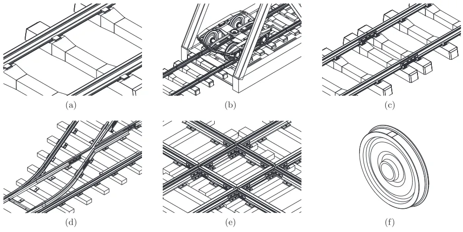
This paper analyses the effect of typical local rail and wheel surface defects as shown in Figure 1. First, a general description of the prediction model, based on a numerical two-step approach, is presented. A vali-dated (Kouroussis et al., 2015) vehicle-track-soil model is studied, based on the AM96 trainset, largely used in Brussels Region (Belgium), for which substantial measured data exists (Kouroussis, Conti and Verlinden, 2013). Different defect geometries and sizes are considered for various train speeds and then their effect on vibration levels analysed.

(a) (b) (c)

(d) (e) (f)

Figure 1. Overview of possible surface defects encountered in practice: (a) reference (no defect), (b) foundation transition, (c) fishplated rail joints, (d) turnout, (e) crossing and (f) wheel flat.

2. Classification of local defects

Figure 2 shows the local rail and wheel surface defect geometries associated with the defects illustrated in Figure 1. For each defect, the geometry and the shape “seen” by the wheel/rail interface are illustrated.

The shape seen accounts for the wheel radiusRwand the vehicle speedv0.

The link between these theoretical shapes (Figure 2) and the physical defects that are present on track is not a one-to-one relationship. Instead, real defects may form a combination of the defects shown. Despite this, some typical cases can be considered:

• Complete switch mechanism (Figure 1(d)) comprises successive step-up joints and pulse joints, e.g.

Figure 2(b) and Figure 2(e).

• Crossings, and diamond crossings as presented in Figure 1(e), are used in double junction and are

defect shape (material geometry of rail or wheel surface)

shape “seen” by the wheel/rail interface (taking into account the wheel curvature of radiusRw)

l

h v0 Rw

(a)

h v0 Rw

(b)

h v0 Rw

(c)

l

h v0 Rw

(d)

l

v0 Rw

(e)

r

v0 Rw

(f)

Figure 2. Mathematical modelling of local rail and wheel surface defects: (a) ramp, (b) step-up joint, (c) step-down joint, (d) pulse joint, (e) negative pulse joint and (f) wheel flat.

• Foundation transition zone (Figure 1(b)) is similar to a ramp which may occur at track–bridge or

ballast–slab track transitions due to a change in track stiffness (Figure 2(a)). A local foundation compaction can induce a variation in height of rail.

• Rail joint (Figure 1(c)) can comprise of any combination of Figures 2(b)–(e). This is dependent upon

the variation in height and in spacing between the two connected rails.

• Wheel flat (Figure 1(f)) is considered as a newly created flat, Figure 2(f).

3. Numerical model

3.1. Fundamental assumptions

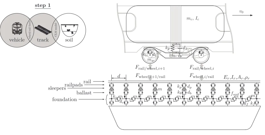
The proposed prediction model is based on two successive calculations and thus facilitates a high accuracy modelling approach for each subsystem. The first step is a vehicle/track analysis. The ballast reactions are then saved and used as input forces for the second step which is a ground wave model. The following assumptions are made:

• Only rigid (multi-)body modes are considered for the vehicle.

• Only vertical dynamic forces are analysed. The vehicle/track model is defined as a bidimensional

problem (in the vertical plane); all the proposed defects are assumed to be symmetrical on each side of the track and in-phase.

• To couple the vehicle and track equations of motion, normal wheel/rail contacts must be expressed. Therefore, the corresponding contact forces are calculated according to non-linear Hertz’s theory. The track and wheel imperfections are included in the contact law.

• At the transition zones (e.g. between the wheel curvature and wheel flat), a small radius is modelled

for the corner between the two profiles, with a value of 0.01Rw to avoid singularities in the contact

zones.

• The vehicle has a constant speedv0for all presented cases.

For the soil modelling, novel soil modelling approaches (e.g. 2.5D modelling (Sheng et al., 2006; Costa et al., 2010; Galvín et al., 2010) and Floquet transforms (Chebli et al., 2008)) are unfeasible due to non-periodicity in the track direction. A three-dimensional approach is therefore necessary.

3.2. Vehicle/track modelling

The dynamics of the vehicle/track subsystem are simulated by considering a multibody vehicle model moving on a flexible track (Figure 3). The wheel/rail forces are defined using Hertz’s theory and allow coupling between the vehicle model and the track. The latter is defined as a flexible beam discretely supported by the sleepers, including viscoelastic elements for the ballast and the railpads. To take into account the dynamic behaviour of the foundation (which plays an important role at low frequencies), a coupled lumped mass model is added to the track model with interconnection elements for the foundation-to-foundation coupling (Kouroussis, Van Parys, Conti and Verlinden, 2013). This model does not take into account other track degrees of freedom. In particular, the sleeper is known to move in a translational and rotational displacements which would expect to produce a more complex excitation. With that in mind, the proposed model is a reasonable approach to take for the study being presented, since it was validated in similar cases (Kouroussis et al., 2012). A C++ object-oriented program was developed using the

in-houseEasyDynlibrary (Verlinden et al., 2013). An application based on aMuPad/Xcasplatform generates

symbolic kinematic expressions for the vehicle. The generalized coordinates approach enables a system of

pure ordinary differential equations, without constraint equations. TheMuPad/Xcasplatform creates a C++

code directly compilable with theEasyDynlibrary. This programmable code is completed by the definition of

applied forces (suspensions, wheel/rail contact) and the link to the track model (which is already established and depends only on site parameters). An implicit scheme is used for the simulation in this first step due to the stiff equations partially obtained for the wheel/rail contact.

3.3. Wheel/rail contact

To couple the vehicle and track equations of motion, normal wheel/rail contacts must be expressed. The corresponding contact forces are calculated according to Hertz’s non-linear theory. The vertical dynamic

forces released by the contact and that act upon each wheeli and on the rail at the coordinatexj can be

written as:

Frail/wheel,i =

 



−KHz(zwheel,i−zrail(xj)−hdefect(xj))3/2 ifzwheel,i>(zrail(xj)−hdefect(xj))

0 otherwise

(1)

= −Fwheel,i/rail (2)

whereKHzis determined from the radii of curvature of the wheel and rail surfaces and the elastic properties of their materials. zwheel,iandzrail(xj) denote the vertical positions of the wheel and of the rail, respectively.

As the vehicle moves along the track at a specific speed v0, the rail contact point changes. The defect

geometry hdefect is calculated from the mathematical shapes defined in Section 2. A 3D finite element

model is first employed to simulate rail and wheel stress and strain distributions in the wheel/rail contact

x x x x x x x x x x x x x x x x x x x x x x x x x x x x x x x x x x x x x x x x x x x x step 1

vehicle wh track soil

ee l/ ra il fo rc e C L M m o d el d rail railpads sleepers ballast foundation

mc,Ic

mb,Ib

mw mf kf kc df dc k1 k2 d1 d2 kp kb dp db v0 fsoil m

Frail/wheel,i

Fwheel,i/rail

Frail/wheel,i+1

Fwheel,i+1/rail _E

r,Ir,Ar,ρr

Figure 3. Description of the prediction model: vehicle/track/foundation simulation.

3.4. Ground wave propagation modelling

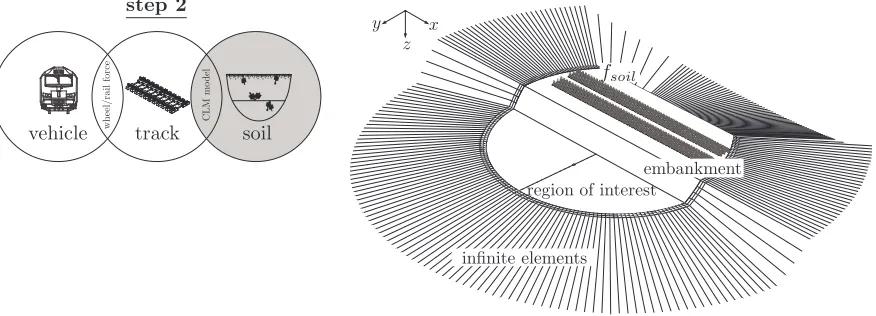
The second step addresses the dynamics of the soil subsystem. Soil surface forces fsoil represent the

contribution from the sleepers (Figure 4). The dynamic ground response is calculated using finite element

methods via the commercial software packageABAQUS. Kouroussis, Van Parys, Conti and Verlinden (2014)

implemented a fully 3D finite element model to optimise finite element method performance and to allow treatment of complex geometry (track embankment, inclined layer interfaces). Moreover, variability in track profile and high ground vibrations originating in singular rail surface defects can be readily analysed. The combined use of viscous boundaries and infinite elements provides more efficient non-reflecting conditions than classical setups (free or fixed boundaries). Here, the small dependence on incident wave angle and dynamic parameters was quantitatively carried out for each solution. A spherical soil border geometry is defined, to which infinite elements are attached. This convex-shape configuration ensures the condition of non-crossing infinite elements. The simulation is performed in the time domain. This is an interesting solution to study ground vibrations in a relatively small area of interest. Since ground vibrations are inherently a transient phenomenon, the time domain analysis is appropriate to simulate wave propagation. It also does not impose any condition on the domain size, which would be required in the frequency domain. Moreover, the equations of motion describing the soil dynamics use an explicit central difference integration scheme to reduce computational burden.

3.5. Environmental impact assessment

A selection of standards/metrics used in Europe and North America were chosen to quantify the influence of vibrations on human perception and damages to buildings (Kouroussis, Conti and Verlinden, 2014), in the range of 1–80 Hz.

ISO standard (International Organization for Standardization, 2003) is dedicated to vibrations felt within a building. In 2013, the evaluation procedure was updated to include frequency-dependent filters related to activity, but was independent of measurement direction and human position (standing, sitting or sleeping). The previous 1989 version of ISO 2631-2 is based on a comparison of the frequency signal with

a third-octave band limit curve. The weighted accelerationaw is derived from the time history of ground

step 2

vehicle wh track soil

ee

l/

ra

il

fo

rc

e

C

L

M

m

o

d

el

x z y

infinite elements

region of interest

embankment

fsoil

Figure 4. Finite element soil modelling using infinite elements and viscous boundary conditions.

vibration amplitude, assuming that the human body responds to an average vibration amplitude between a

recorded time of 0≤t≤T

hawi=

s

1

T

Z T

0

a2

w(t) dt . (3)

Guidelines on the effect of vibration on comfort and perception are provided and limits are used to define vibration thresholds.

Alternatively, as vibration is often non-stationary, DIN 4150-2

stan-dard (Deutsches Institut für Normung, 1999a) proposes the use of a running, root-mean square applied to the velocity signal. A weighted, time-averaged signal is defined by:

KBF(t) =

s

1

τ

Z t

0

KB2_(ξ)e−t−τξdξ (4)

where the weighted velocity signalKB(t) is obtained by passing the original ground vibration velocity signal

v(t) through the high-pass filter

HKB(f) = p 1

1 + (5.6/f)2 . (5)

The filter is a function of the frequency f. The assimilation time τ is typically equal to 0.125 s, which

takes into account transient phenomena, such as impacts or shocks, that would otherwise be masked if a simple operation is performed. The only comfort that can then be assessed is by comparing the

maximum level KBF,max with three guideline limits denoted by Au, Ao and Ar. Part 3 of DIN

4150-3 (Deutsches Institut für Normung, 1999b) is entirely dedicated to structural vibrations. The peak particle

velocityP P V, which is defined as the maximum absolute amplitude of the velocity time signal, is calculated

and compared to other limits, dependent upon the dominant signal frequency. If multiple directions are

measured, the maximum of the three components (x, y orz) is

P P V = max(|vx|,|vy|,|vz|). (6)

In addition to Eq. (6), when the three components are of the same order of magnitude, the norm of the vector velocity can be used, as suggested by the Swiss standard (Schweizerische Normen-Vereinigung, 1992)

P P V = qv2

Taking into account that vibrations exist over a wide range of amplitudes, the U.S. Department of Transportation adopted a decibel scale in order to evaluate the vibrational impact of a passing high-speed train (U. S. Department of Transportation, 1998). This is similar to how noise is measured and compresses the range of numbers required to describe the vibration velocity level. It is defined as:

VdB = 20 log10

vrms 5 10−8 [m/s]

(8)

wherevrmsis the root mean square amplitude of the velocity time history. Note that no weighting is applied

to the signal, which is contrary to ISO standards.

4. Numerical simulations and results

Local defects are often encountered by urban trains. Therefore, this study focuses on the

Inter-City train operating in Brussels (Belgium). The AM96 trainset, largely used by the Belgian

Rail-way Operator, SNCB, is typically used for InterCity and InterRegion connections. This study evalu-ates the AM96 trainset’s generation of elevated ground vibration levels in comparison to other domestic trains (Kouroussis, Conti and Verlinden, 2013). It consists of three carriages, designated HVBX, HVB, and HVADX. The HVBX leading wagon is equipped with motorised bogies, whereas the HVB (middle) and HVADX (end) wagons are trailer carriages. Figure 5 shows the configurations and the positions of each wheelset on the vehicle. A classical multibody approach is used and limits the vehicle dynamics to pitch and bounce motions. Table 1 presents the dynamic and geometrical informations of each carriage. Track and soil data are provided in Tables 2 and 3, respectively. This vehicle configuration has been recently validated using free field measurements (Kouroussis et al., 2015).

HVBX HVB HVADX

3.70 3.70

2.56 2.56

2.56 2.56 2.56

2.56

4.00

4.00 4.00

4.00

26.40 26.40

26.40

18.40 18.70

18.70

Figure 5. Configuration of the AM96 electric multiple unit.

Table 1. Dynamic parameters of AM96 vehicle — unladen weight (Kouroussis, Connolly and Verlinden, 2014).

HVB HVADX HVBX

Car body mass 25200 kg 28900 kg 25932 kg

Bogie mass 6900 kg 7050 kg 11800 kg

Wheelset mass 1700 kg 1700 kg 2375 kg

Car body radius of gyration 7.09 m 7.09 m 7.09 m

Bogie radius of gyration 0.47 m 0.47 m 0.47 m

Bogie spacing 15.84 m 15.84 m 15.84 m

Wheelset spacing 2.56 m 2.56 m 2.56 m

Primary suspension stiffness 1.30 MN/m 1.30 MN/m 1.81 MN/m

Primary suspension damping 3.7 kNs/m 3.7 kNs/m 1.14 kNs/m

Secondary suspension stiffness 0.69 MN/m 0.69 MN/m 0.69 MN/m

Table 2. Parameters of the track at Watermael (Brussels Region — Belgium).

Rail flexural stiffness 6.42 MNm2

Rail mass per length 60 kg/m

Sleeper spacing 0.6 m

Sleeper mass 150 kg

Railpad stiffness 550 MN/m

Railpad damping coefficient 68 kNs/m

Ballast stiffness 361 MN/m

Ballast damping coefficient 55 kNs/m

Table 3. Summary of the dynamic soil characteristics at site of Watermael (Brussels Region — Belgium).

Layer top bottom bank

material

alluvium

sand of Brussels

sand and clay of Ypres

layer 1

layer 2

angle of inclination 18o

Young’s modulus 120 MN/m2 _{500 MN/m}2

Density 1600 kg/m3 _{2500 kg/m}3

Poisson’s ratio 0.3 0.3

Compression wave velocity 320 m/s 520 m/s

Shear wave velocity 171 m/s 278 m/s

Viscous damping 0.0004 s 0.0004 s

4.1. Free-field ground vibrations

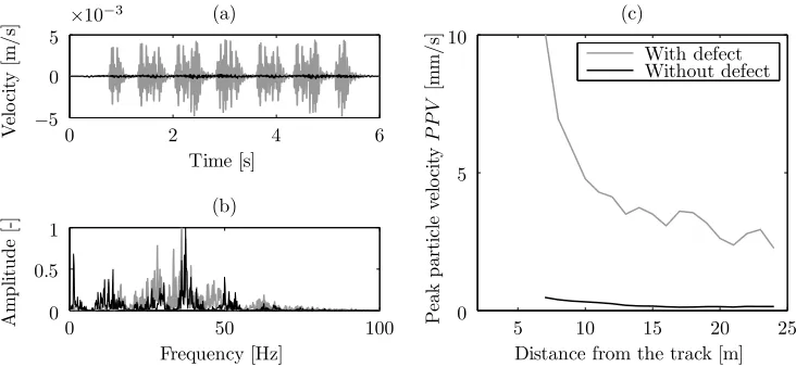
Figure 6 presents numerical results, for the case of no defect and also a ramp irregularity (vertical

height h= 5 mm and horizontal length l = 200 mm). The AM96 trainset runs at a speedv0 of 120 km/h.

The comparison is based on the time history of numerical velocities in the vertical direction (Figure 6(a)) and the corresponding normalized frequency content (Figure 6(b)), both for a distance of 10 m from the track. A significant difference in levels is observed between the two cases’ velocity traces (more than ten times magnification), thus showing the significant contribution of local irregularities to vibration levels. The passing of each wheelset is more clearly pronounced in the case where the defect is present.

(a) Time [s] V el o ci ty [m /s ]

0 2 4 6

×10−3

−5 0 5 (b) Frequency [Hz] Am p li tu d e [-]

0 50 100

0 0.5 1

Distance from the track [m]

P eak p ar ti cl e ve lo ci ty P P V [m m /s ] (c)

5 10 15 20 25

0 5 10

With defect Without defect

Figure 6. Comparison between numerical data (grey: with 5 mm height/200 mm length ramp defect; black: without defect) related to the passage of an AM96 trainset (2×3 carriages) at a speedv0of 120 km/h: (a) time histories at 10 m from the track, (b) normalised frequency contents at 10 m from the track and (c) peak particle velocity as a function of the distance from the track.

frequencies are located in the frequency range 0 – 60 Hz. Several dominant frequencies due to the fundamental and harmonic carriage frequencies are present and are a multiple of

fc= v0

Lc

(9)

where Lc is the carriage length. In addition, the fundamental axle and bogie passage frequencies imply a

double amplitude modulation, as discussed in (Kouroussis, Connolly and Verlinden, 2014):

fa= v0

La

(10)

fb= v0

Lb

(11)

where La is the wheelset spacing, and Lb the bogie spacing. In the studied case (fa = 13 Hz and fb =

1.8 Hz), the axle frequency modulation is clearly visible on both spectra (i.e. at 6.5 Hz, 19.5 Hz, 32.5 Hz,

45.5 Hz and 58.5 Hz where the magnitude is close to zero). This modulation effect is also visible on the

dominant frequencies n fc. More importantly, it is seen that the presence of the local defect amplifies

the frequency magnitude between 20 Hz and 60 Hz. In this large range, the soil resonance also plays a role (Kouroussis et al., 2015).

Figure 6(c) shows the far field peak particle velocity P P V defined by Eq. (6). The analysis is based

on a track with an embankment: receivers are placed outside the embankment area (in the far field) where

ground vibration is most likely problematic. The ground vibration level decreases with the distancedfrom

the track and the decay rate is different when the defect is present. Without the defect it is approximately

d−0.9; however, with the defect, it reaches upd−1.2. Interestingly, the decay rate is then outside the power

law range [0.5–1.1] proposed by Auersch and Said (2010).

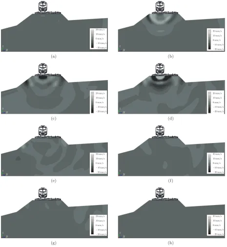
Figure 7 shows a cross section of the ground wave propagation for the same defect case, thus giving a comprehensive view of the free field response on the soil’s surface. The selected time histories show the

instants when the first bogie crosses the local defect (beginning of the ramp). At t < 0.75 s, the ground

wave generation is due to the quasi-static contribution of the vehicle (no contact with the local defect). At

t >0.75 s, the ground wave propagation is amplified by the wheel/defect contact due to the vehicle/track

dynamics. This effect is visible until t = 1 s, showing that the phenomenon is transient and affects each

wheel/defect impact. It is noteworthy that the embankment plays a role in the ground wave propagation by trapping wave guide for railway vibrations (clearly visible in Figures 7(c) and (d)). This results in increased vibration levels inside the embankment and was also found by Connolly, Giannopoulos and Forde (2013).

4.2. The influence of defect type

The six shapes of discontinuity presented in Figure 2 (representing various defect types such as transition zones, switches, crossings, rail joints, and wheel flats) are analysed in this section. Again, the vehicle is the

AM96 trainset running at a constant speedv0.

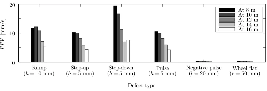
Figure 8 presents the surface ground vibration levels at different distances from the track, outside the embankment. The values of defect length and size were selected according to those found in practice. For the ramp function, the lengthlis 200 mm (sufficiently long to replicate a small transition zone with a slope of

3o_{) and heighth= 10 mm. For the pulse function, the length is fixed atl= 10 mm with a heighth= 5 mm.}

For the negative pulse function, the length is fixed atl= 20 mm. For the other rail defects, only the height

intervenes, fixed toh= 5 mm. The wheel flat spot has a lengthr= 50 mm.

z y

0 mm/s 10 mm/s 20 mm/s

−10 mm/s −20 mm/s

(a)

z y

0 mm/s 10 mm/s 20 mm/s

−10 mm/s −20 mm/s

(b)

z y

0 mm/s 10 mm/s 20 mm/s

−10 mm/s −20 mm/s

(c)

z y

0 mm/s 10 mm/s 20 mm/s

−10 mm/s −20 mm/s

(d)

z y

0 mm/s 10 mm/s 20 mm/s

−10 mm/s −20 mm/s

(e)

z y

0 mm/s 10 mm/s 20 mm/s

−10 mm/s −20 mm/s

(f)

z y

0 mm/s 10 mm/s 20 mm/s

−10 mm/s −20 mm/s

(g)

z y

0 mm/s 10 mm/s 20 mm/s

−10 mm/s −20 mm/s

(h)

Figure 7. Numerical visualisation (x-axis planar view — vertical velocityvz) of the passage of an AM96 trainset at a speed of

120 km/h on a 5 mm height ramp defect: free field vertical component of the soil vibration waves (a) at 0.7 s, (b) at 0.75 s, (c) at 0.8 s, (d) at 0.85 s, (e) at 0.9 s, (f) at 0.95 s, (g) at 1.0 s , (h) at 1.05 s.

opposite in shape). The ramp function also presents large vibration levels although it represents a priori a small variation in height. Very small levels of vibration are observed for the negative pulse and wheel flat, and are close to those obtained in the absence of local defects (not presented here). Finally, the decrease

Defect type

P

P

V

[m

m

/

s]

Ramp Step-up Step-down Pulse Negative pulse Wheel flat

0 10 20

At 8 m At 10 m At 12 m At 14 m At 16 m

(h_{= 10 mm) (}h_{= 5 mm) (}h_{= 5 mm) (}h_{= 5 mm) (}l_{= 20 mm) (}r_{= 50 mm)}

Figure 8. Peak particle velocity as a function of the distance from the source and the defect type for an AM96 trainset running at 120 km/h.

occur with distance.

4.3. The influence of defect size

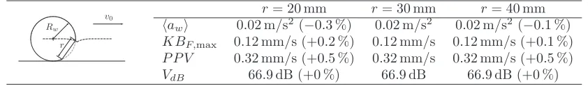
A sensitivity analysis is presented in Tables 4 through 9 for when the primary defect dimension varies (h

for the ramp, the step-up joint, the step-down joint, the pulse joint;lfor the negative pulse joint;r for the wheel flat). The four aforementioned indicators (accelerationhawiand velocitiesP P V,KBF,max andVdB) are used to quantify the variation in ground vibration level. In general, there was found to be a positive relationship between each indicator and defect size. Despite this, the relationship between size and vibration level was not linear due to the non-linear effect of the wheel/rail contact. In addition, for some defects (e.g. step-down joint), the size was found to be very influential on defect size.

Table 4. Ground vibration level at 10 m from the source for an AM96 trainset running at 120 km/h on a ramp.

h= 5 mm h= 10 mm h= 15 mm

l h v0

Rw

l= 200 mm l= 200 mm l= 200 mm

hawi 0.37 m/s2(−56 %) 0.84 m/s2 1.15 m/s2(+37 %)

KBF,max 2.26 mm/s (−57 %) 5.29 mm/s 7.22 mm/s (+36 %)

P P V 4.78 mm/s (−61 %) 12.23 mm/s 20.64 mm/s (+69 %)

VdB 90.7 dB (−8 %) 98.1 dB 101.0 dB (+3 %)

Table 5. Ground vibration level at 10 m from the source for an AM96 trainset running at 120 km/h on a step-up joint.

h v0

Rw

h= 2.5 mm h= 5 mm h= 7.5 mm

hawi 0.35 m/s2(−47 %) 0.67 m/s2 0.78 m/s2(+17 %)

KBF,max 1.95 mm/s (−57 %) 4.54 mm/s 5.06 mm/s (+11 %)

P P V 4.29 mm/s (−57 %) 10.01 mm/s 11.43 mm/s (+14 %)

VdB 89.8 dB (−7 %) 96.2 dB 97.3 dB (+1 %)

At 120 km/h, the wheel flat and negative pulse have an insignificant effect on ground vibrations. In

general, this is due to the vehicle speed shifting the frequency content to a higher range. These high frequencies are then rapidly dampened by the soil and the track, meaning that, at the studied distances,

their effect is insignificant. Figure 9 illustrates this by comparing the soil surface P P V generated by the

Table 6. Ground vibration level at 10 m from the source for an AM96 trainset running at 120 km/h on a step-down joint.

h v0

Rw

h= 2.5 mm h= 5 mm h= 7.5 mm

hawi 0.14 m/s2(−66 %) 0.42 m/s2 0.88 m/s2(+108 %)

KBF,max 0.84 mm/s (−86 %) 6.22 mm/s 10.40 mm/s (+67 %)

P P V 2.13 mm/s (−87 %) 16.69 mm/s 28.49 mm/s (+71 %)

VdB 81.7 dB (−15 %) 96.1 dB 102.2 dB (+6 %)

Table 7. Ground vibration level at 10 m from the source for an AM96 trainset running at 120 km/h on a pulse joint.

h= 2.5 mm h= 5 mm h= 7.5 mm

l h v0

Rw

l= 10 mm l= 10 mm l= 10 mm

hawi 0.36 m/s2 (−51 %) 0.73 m/s2 0.72 m/s2 (−1 %) KBF,max 1.93 mm/s (−57 %) 4.51 mm/s 4.50 mm/s (−0.1 %)

P P V 4.06 mm/s (−59 %) 10.00 mm/s 10.31 mm/s (+3 %)

VdB 89.6 dB (−7 %) 96.5 dB 97.6 dB (+0.1 %)

Table 8. Ground vibration level at 10 m from the source for an AM96 trainset running at 120 km/h on a negative pulse joint.

l v0

Rw

l= 10 mm l= 20 mm l= 30 mm

hawi 0.02 m/s2(+0.3 %) 0.02 m/s2 0.02 m/s2(−0.7 %) KBF,max 0.12 mm/s (+0.6 %) 0.12 mm/s 0.12 mm/s (−1 %)

P P V 0.32 mm/s (−0.4 %) 0.32 mm/s 0.32 mm/s (+1 %)

VdB 66.9 dB (+0 %) 66.9 dB 66.8 dB (−0.2 %)

Table 9. Ground vibration level at 10 m from the source for an AM96 trainset running at 120 km/h with a wheel flat.

r

v0

Rw

r= 20 mm r= 30 mm r= 40 mm

hawi 0.02 m/s2(−0.3 %) 0.02 m/s2 0.02 m/s2(−0.1 %) KBF,max 0.12 mm/s (+0.2 %) 0.12 mm/s 0.12 mm/s (+0.1 %)

P P V 0.32 mm/s (+0.5 %) 0.32 mm/s 0.32 mm/s (+0.5 %)

VdB 66.9 dB (+0 %) 66.9 dB 66.9 dB (+0 %)

the difference between the different cases, as observed in the near-field embankment area. In Figure 9(a), the reference case without a defect is shown and Figure 9(b) shows the case for a defect generating large amplitude vibrations (5 mm height step-up joint defect). The negative pulse defect and wheel flat defect cases are also presented (Figures 9(c) and (d)) because there are associated to relatively low ground vibration levels. For both defects, the ground vibration level is very close to the reference case, except in the vicinity of the track where a discrepancy is found. This is because the periodic effect of wheel flat impact affects the track while the effect of the negative pulse defect affects a close area localised around the geometrical defect. Regarding the vibration field generated by the step-up joint defect, it is similar to those generated by a stationary point load (spherical-like ground wave shapes). Therefore this implies that the longitudinal position of the defect is important in the assessment of vibration annoyance in addition to distance from the track.

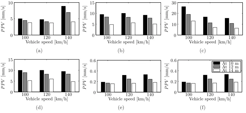
4.4. The influence of vehicle speed

Figure 10 presents, the variation inP P V for several distances from the track, for each defect, for speeds

v0= 100 km/h, 120 km/h and 140 km/h. Note that the two defects — negative pulse joint and wheel flat —

x y

0 mm/s 5 mm/s 15 mm/s 10 mm/s 20 mm/s track

(a)

x y

0 mm/s 5 mm/s 15 mm/s 10 mm/s 20 mm/s

track

(b)

x y

0 mm/s 5 mm/s 15 mm/s 10 mm/s 20 mm/s track

(c)

x y

0 mm/s 5 mm/s 15 mm/s 10 mm/s 20 mm/s track

(d)

Figure 9. Birdseye track view (P P V according to Eq. (7)) during the passage of an AM96 trainset at a speed of 120 km/h (a) without defect (static contribution), (b) with a 5 mm height step-up joint defect, (c) with a 40 mm length negative pulse defect and (d) with a 50 mm flat spot.

Vehicle speed [km/h]

P P V [m m / s]

100 120 140

0 5 10

(a)

Vehicle speed [km/h]

P P V [m m / s]

100 120 140

0 5 10 15

(b)

Vehicle speed [km/h]

P P V [m m / s]

100 120 140

0 10 20 30

(c)

Vehicle speed [km/h]

P P V [m m / s]

100 120 140

0 5 10 15

(d)

Vehicle speed [km/h]

P P V [m m / s]

100 120 140

0 0.₂

0.₄

0.₆

(e)

Vehicle speed [km/h]

P P V [m m / s]

100 120 140

0 0.₂

0.₄

0.₆

At 10 m At 12 m At 14 m

(f)

Figure 10. Peak particle velocity as a function of the vehicle speed for an AM96 trainset running on (a) ramp (l= 200 mm,

h= 5 mm), (b) step-up joint (h= 5 mm), (c) step-down joint (h= 5 mm), (d) pulse joint (h= 5 mm), (e) negative pulse joint (l= 10 mm) and (f) wheel flat (r= 50 mm).

vibration levels always increase with the vehicle speed. To understand this, it is useful to note that in previous studies, vibration levels were calculated using numerical and experimental observations where only quasi-static effects (moving load along the track) were coupled to a distributed overall unevenness (dynamic effect). In this case, local defects are considered rather than continuous defects, and thus generate different dynamic effects due to the contrast in the vehicle/track interaction. This changes the frequency response of the system, which may also be subject to carriage modulation effects (i.e. the frequency content generated by the defect impact may be magnified if it is inside the lobes defined by the axle periodicity).

5. Conclusion

The effect of railway track local irregularities (discontinuities) on ground-vibration levels was analysed. A time domain vibration prediction model was used to investigate vibration levels generated at the wheel/rail contact due to a variety of defects, including rail joints, switches, crossings and wheel flats. This was advantageous because when simulating transient events such as the forces generated in the contact zone between wheel and track discontinuities, time domain modelling is better suited than most frequency domain approaches. The prediction of 4 international metrics (hawi,KBF,max,P P V andVdB) was considered, and a sensitivity analysis was undertaken based upon the defect size and train speed. The key findings were:

• Local defects generate large amplitude excitations in comparison to a typical smooth railway track.

• The rate of vibration decay with the distance differs in the presence of a local defect. For the soil

stratum modelled in this work, the decay rate was lower than that usually predicted by previous studies. Therefore it is possible for the vibrations from a defect to propagate to elevated distances in comparison to typical railway vibration

• Defect type has a significant influence on vibration levels. Step-down joints typically associated with

switch/crossings generate the highest level of vibration, whereas negative pulse joints, and wheel flats generate the lowest.

• Defect geometry influences vibration levels and, in general, an increasing defect size causes increasing

vibration levels.

• The relationship between defect type and train speed in complex. For some defects, vibration levels

increase with speed, however for other types it decreases.

References

Alexandrou, G., Kouroussis, G. and Verlinden, O. (2015). A comprehensive prediction model for vehicle/track/soil dynamic response due to wheel flats,Journal of Rail and Rapid Transitin press, doi: 10.1177/0954409715576015.

Andersson, C. and Oscarsson, J. (1999). Dynamic train/track interaction including state-dependent track properties and flexible vehicle components,Vehicle System Dynamics33(supplement): 47–58.

Auersch, L. and Said, S. (2010). Attenuation of ground vibrations due to different technical sources,Earthquake Engineering and Engineering Vibration9: 337–344.

Chebli, H., Clouteau, D. and Schmitt, L. (2008). Dynamic response of high-speed ballasted railway tracks: 3D periodic model and in situ measurements,Soil Dynamics and Earthquake Engineering28(2): 118–131.

Connolly, D., Giannopoulos, A., Fan, W., Woodward, P. and Forde, M. (2013). Optimising low acoustic impedance back-fill material wave barrier dimensions to shield structures from ground borne high speed rail vibrations,Construction and Building Materials44: 557–564.

Connolly, D., Giannopoulos, A. and Forde, M. C. (2013). Numerical modelling of ground borne vibrations from high speed rail lines on embankments,Soil Dynamics and Earthquake Engineering46: 13–19.

Connolly, D. P., Costa, P. A., Kouroussis, G., Galvín, P., Woodward, P. K. and Laghrouche, O. (2015). Large scale international testing of railway ground vibrations across europe,Soil Dynamics and Earthquake Engineering71: 1–12.

Connolly, D. P., Kouroussis, G., Laghrouche, O., Ho, C. and Forde, M. C. (2014). Benchmarking railway vi-brations — track, vehicle, ground and building effects, Construction and Building Materials in press, doi: 10.1016/j.conbuildmat.2014.07.042.

Connolly, D. P., Kouroussis, G., Woodward, P. K., Verlinden, O., Giannopoulos, A. and Forde, M. C. (2014). Scoping prediction of re-radiated ground-borne noise and vibration near high speed rail lines with variable soils,Soil Dynamics and Earthquake Engineering66: 78–88.

Costa, P. A., Calçada, R., Cardoso, A. S. and Bodare, A. (2010). Influence of soil non-linearity on the dynamic response of high–speed railway tracks,Soil Dynamics and Earthquake Engineering30(4): 221 – 235.

Costa, P. A., Calçada, R. and Cardoso, A. S. (2012). Influence of train dynamic modelling strategy on the prediction of track–ground vibrations induced by railway traffic,Journal of Rail and Rapid Transit226(4): 434–450.

Coulier, P., François, S., Degrande, G. and Lombaert, G. (2013). Subgrade stiffening next to the track as a wave impeding barrier for railway induced vibrations,Soil Dynamics and Earthquake Engineering48: 119–131.

Degrande, G. and Schillemans, L. (2001). Free field vibrations during the passage of a Thalys high-speed train at variable speed,Journal of Sound and Vibration247(1): 131–144.

Deutsches Institut für Normung (1999a). DIN 4150-2: Structural vibrations — Part 2: Human exposure to vibration in buildings.

Deutsches Institut für Normung (1999b). DIN 4150-3: Structural vibrations — Part 3: Effects of vibration on structures. Galvín, P. and Domínguez, J. (2009). Experimental and numerical analyses of vibrations induced by high-speed trains on the

Córdoba–Málaga line,Soil Dynamics and Earthquake Engineering29: 641–651.

Galvín, P., François, S., Schevenels, M., Bongini, E., Degrande, G. and Lombaert, G. (2010). A 2.5D coupled FE-BE model for the prediction of railway induced vibrations,Soil Dynamics and Earthquake Engineering30(12): 1500–1512.

Garinei, A., Risitano, G. and Scappaticci, L. (2014). Experimental evaluation of the efficiency of trenches for the mitigation of train-induced vibrations,Transportation Research Part D: Transport and Environment32(0): 303–315.

Grossoni, I., Iwnicki, S., Bezin, Y. and Gong, C. (2015). Dynamics of a vehicle–track coupling system at a rail joint,Journal of Rail and Rapid Transit229(4): 364–374.

International Organization for Standardization (2003). ISO 2631-2: Mechanical vibration and shock — Evaluation of human exposure to whole-body vibration — Part 2: Vibration in buildings (1 to 80 Hz).

Kouroussis, G., Connolly, D. P. and Verlinden, O. (2014). Railway induced ground vibrations — a review of vehicle effects, International Journal of Rail Transportation2(2): 69–110.

Kouroussis, G., Conti, C. and Verlinden, O. (2013). Experimental study of ground vibrations induced by Brussels IC/IR trains in their neighbourhood,Mechanics & Industry14(02): 99–105.

Kouroussis, G., Conti, C. and Verlinden, O. (2014). Building vibrations induced by human activities: a benchmark of existing standards,Mechanics & Industry15(5): 345–353.

Kouroussis, G., Florentin, J. and Verlinden, O. (2015). Ground vibrations induced by intercity/interregion trains: A numerical prediction based on the multibody/finite element modeling approach, Journal of Vibration and Controlin press, doi: 10.1177/1077546315573914.

Kouroussis, G., Gazetas, G., Anastasopoulos, I., Conti, C. and Verlinden, O. (2011). Discrete modelling of vertical track–soil coupling for vehicle–track dynamics,Soil Dynamics and Earthquake Engineering31(12): 1711–1723.

Kouroussis, G., Pauwels, N., Brux, P., Conti, C. and Verlinden, O. (2014). A numerical analysis of the influence of tram characteristics and rail profile on railway traffic ground-borne noise and vibration in the brussels region,Science of the Total Environment482-483: 452–460.

Kouroussis, G., Van Parys, L., Conti, C. and Verlinden, O. (2013). Prediction of ground vibrations induced by urban railway traffic: an analysis of the coupling assumptions between vehicle, track, soil, and buildings,International Journal of Acoustics and Vibration18(4): 163–172.

Kouroussis, G., Van Parys, L., Conti, C. and Verlinden, O. (2014). Using three-dimensional finite element analysis in time domain to model railway–induced ground vibrations,Advances in Engineering Software70: 63–76.

Kouroussis, G. and Verlinden, O. (2015). Prediction of railway ground vibrations: accuracy of a coupled lumped mass model for representing the track/soil interaction,Soil Dynamics and Earthquake Engineering69: 220–226.

Kouroussis, G., Verlinden, O. and Conti, C. (2012). Efficiency of resilient wheels on the alleviation of railway ground vibrations, Journal of Rail and Rapid Transit226(4): 381–396.

Madshus, C. and Kaynia, A. M. (2000). High-speed railway lines on soft ground: dynamic behaviour at critical train speed, Journal of Sound and Vibration231(3): 689–701.

Mandal, N. K., Dhanasekar, M. and Sun, Y. Q. (2014). Impact forces at dipped rail joints,Journal of Rail and Rapid Transit

in press, doi: 10.1177/0954409714537816.

Nielsen, J. C. O. and Abrahamsson, T. J. S. (1992). Coupling of physical and modal components for analysis of moving non-linear dynamic systems on general beam structures,International Journal for Numerical Methods in Engineering33(9): 1843–1859. Nielsen, J. C. O., Mirza, A., Cervello, S., Huber, P., Müller, R., Nelain, B. and Ruest, P. (2015). Reducing train-induced

ground-borne vibration by vehicle design and maintenance,International Journal of Rail Transportation3(1): 17–39. Oscarsson, J. and Dahlberg, T. (1998). Dynamic train/track/ballast interaction - computer models and full-scale experiments,

Vehicle System Dynamics29(supplement): 73–84.

Paixão, A., Fortunato, E. and Calçada, R. (2015). Design and construction of backfills for railway track transition zones, Journal of Rail and Rapid Transit229(1): 58–70.

Schweizerische Normen-Vereinigung (1992). SN-640312a: Les ébranlements — Effet des ébranlements sur les constructions [Swiss Standard on vibration effects on buildings].

Sheng, X., Jones, C. J. C. and Thompson, D. J. (2006). Prediction of ground vibration from trains using the wavenumber finite and boundary element methods,Journal of Sound and Vibration293(3–5): 575–586.

U. S. Department of Transportation (1998). High-speed ground transportation. Noise and vibration impact assessment, Tech-nical Report 293630–1, Office of Railroad Development Washington (Federal Railroad Administration).

Uzzal, R. U. A., Ahmed, W. and Bhat, R. B. (2014). A three-dimensional modeling study of wheel/rail impacts created by multiple wheel flats, and the development of a smart wheelset, Journal of Rail and Rapid Transit in press, doi: 10.1177/0954409714545558.

Verlinden, O., Ben Fekih, L. and Kouroussis, G. (2013). Symbolic generation of the kinematics of multibody systems in EasyDyn: from MuPAD to Xcas/Giac,Theoretical & Applied Mechanics Letters3(1): 013012.

Vogiatzis, K. (2010). Noise and vibration theoretical evaluation and monitoring program for the protection of the Ancient “Kapnikarea Church” from Athens metro operation,International Review of Civil Engineering1: 328–333.

Vogiatzis, K. (2012). Protection of the cultural heritage from underground metro vibration and ground-borne noise in Athens centre: The case of the Kerameikos archaeological museum and Gazi cultural centre,International Journal of Acoustics and Vibration17: 59–72.

Younesian, D., Marjani, S. R. and Esmailzadeh, E. (2014). Importance of flexural mode shapes in dynamic analysis of high-speed trains traveling on bridges,Journal of Vibration and Control20(10): 1565–1583.

Zhai, W. and Sun, X. (1994). A detailed model for investigating vertical interaction between railway vehicle and track,Vehicle System Dynamics23(supplement): 603–615.

Zhai, W., Xia, H., Cai, C., Gao, M., Li, X., Guo, G., Zhang, N. and Wang, K. (2013). High-speed train–track–bridge dynamic interactions — Part I: theoretical model and numerical simulation,International Journal of Rail Transportation1(1-2): 3–24. Zhao, X., Li, Z. and Liu, J. (2012). Wheel–rail impact and the dynamic forces at discrete supports of rails in the presence of