Reasoning about topological and cardinal direction relations between 2-dimensional spatial objects

White Rose Research Online URL for this paper:

http://eprints.whiterose.ac.uk/83876/

Version: Published Version

Article:

Cohn, AG, Li, S, Liu, W et al. (1 more author) (2014) Reasoning about topological and

cardinal direction relations between 2-dimensional spatial objects. Journal of Artificial

Intelligence Research, 51. 493 - 532. ISSN 1076-9757

https://doi.org/10.1613/jair.4513

[email protected] https://eprints.whiterose.ac.uk/ Reuse

Unless indicated otherwise, fulltext items are protected by copyright with all rights reserved. The copyright exception in section 29 of the Copyright, Designs and Patents Act 1988 allows the making of a single copy solely for the purpose of non-commercial research or private study within the limits of fair dealing. The publisher or other rights-holder may allow further reproduction and re-use of this version - refer to the White Rose Research Online record for this item. Where records identify the publisher as the copyright holder, users can verify any specific terms of use on the publisher’s website.

Takedown

If you consider content in White Rose Research Online to be in breach of UK law, please notify us by

Reasoning about Topological and Cardinal Direction Relations

Between 2-Dimensional Spatial Objects

Anthony G. Cohn [email protected]

School of Computing, University of Leeds, UK Faculty of Engineering and Information Technology, University of Technology Sydney, Australia

Sanjiang Li [email protected]

AMSS-UTS Joint Research Lab,

Centre for Quantum Computation & Intelligent Systems, University of Technology Sydney, Australia

College of Computer Science, Shaanxi Normal University, China

Weiming Liu [email protected]

Baidu (China) Co., Ltd., Shanghai, China

Jochen Renz [email protected]

Research School of Computer Science, The Australian National University, Australia

Abstract

Increasing the expressiveness of qualitative spatial calculi is an essential step towards meeting the requirements of applications. This can be achieved by combining existing calculi in a way that we can express spatial information using relations from multiple calculi. The great challenge is to develop reasoning algorithms that are correct and complete when reasoning over the combined information. Previous work has mainly studied cases where the interaction between the combined calculi was small, or where one of the two calculi was very simple. In this paper we tackle the important combination of topological and directional information for extended spatial objects. We combine some of the best known calculi in qualitative spatial reasoning, the RCC8 algebra for representing topological information, and the Rectangle Algebra (RA) and the Cardinal Direction Calculus (CDC) for directional information. We consider two different interpretations of the RCC8 algebra, one uses a weak connectedness relation, the other uses a strong connectedness relation. In both interpretations, we show that reasoning with topological and directional information is de-cidable and remains in NP. Our computational complexity results unveil the significant differences between RA and CDC, and that between weak and strong RCC8 models. Take the combination of basic RCC8 and basic CDC constraints as an example: we show that the consistency problem is in P only when we use the strong RCC8 algebra and explicitly know the corresponding basic RA constraints.

1. Introduction

& Mark, 1995), sea navigation (Wolter et al., 2008), to high level interpretation of video data (Srid-har, Cohn, & Hogg, 2011; Cohn, Renz, & Srid(Srid-har, 2012). We refer the reader to the work of Cohn and Renz (2008), and Wolter and Wallgr¨un (2012) for more information.

The qualitative approach usually represents spatial information by introducing a relation model on the domain of spatial entities, which could be points, line segments, rectangles, or arbitrary regions. In the literature, such a relation model is often called a qualitative calculus(Ligozat & Renz, 2004), which contains a finite set of jointly exhaustive and pairwise disjoint (JEPD) relations defined on the domain. In the past three decades, dozens of spatial relation models have been proposed in the literature (Cohn & Renz, 2008; Chen, Cohn, Liu, Wang, Ouyang, & Yu, 2013). Many of these qualitative calculi approximate spatial entities by points. While this is convenient when representing spatial direction, distance and positions (providing the extent of the objects is small compared to their distance apart), it is inappropriate as far as the shapes and/or topology of the spatial objects are concerned. In this paper, we represent spatial entities as 2-dimensional bounded regions in the real plane, which may have holes or multiple connected components.

In the literature, most spatial calculi focus on one single aspect of space, e.g. topology, direc-tion, distance, posidirec-tion, or shape. Topological relations are those relations that are invariant under homeomorphisms such as scale, rotation, and translation. It is widely acknowledged that topolog-ical relations are of crucial importance. One influential formalism for topologtopolog-ical relations is the region connection calculus (RCC) (Randell, Cui, & Cohn, 1992). Based on one primitive binary connectedness relation, a set of eight JEPD topological relations can be defined in the RCC. This calculus is known as the RCC8 algebra. According to different interpretations of connectedness, this calculus may have different variants. In this paper, we say two (closed) regions areweakly con-nectedif they share at least a common point, and say they arestrongly connectedif their intersection is at least one-dimensional. Accordingly, we address the two resulting RCC8 algebras as the weak and the strong RCC8 algebras respectively. For convenience, we denote the weak RCC8 algebra as RCC8, and the strong one as RCC8′.

The importance of the distinction between strong and weak RCC8 becomes clear when analysing the different ways of defining the neighbourhood of pixels commonly used in Computer Vision. 4-connectedness refers to the pixels that are horizontally and vertically connected to a pixel, while 8-connectedness includes the diagonally neighbouring pixels as well. This distinction corresponds nicely to the distinction between strong and weak RCC8 as 8-connectedness considers connec-tions at a point, while 4-connectedness only considers connecconnec-tions along a line (which is one-dimensional). Therefore, we can use strong or weak RCC8 in a similar way we use 4- or 8-connectedness, depending on the requirements of the application at hand.

The RCC8 algebra only represents topological information between spatial objects. In many practical applications, however, other kinds of relations are often used together with topological relations. For example, when recommending a restaurant you dined at before it is common to give descriptions such as “the restaurant isinthe city centre,west ofthe central station, andnearbythere is a McDonald’s.”

minimum bounding rectangles (MBRs), and relates the two objects by the interval relations between the projected intervals. On the other hand, CDC only approximates the reference object by its MBR, while leaving the primary object unchanged. The CDC has 511 basic relations, and RA has 169 basic relations. Most (487 out of 511) basic CDC relations intersect with one and only one basic RA relation and, hence, are contained in a unique basic RA relation. Therefore, CDC is in a sense more expressive than RA.

A central reasoning problem in QSR is theconsistency problem. An instance of the consistency problem is a setΓof constraints like(xαy), wherex, yare spatial variables, andαis a qualitative relation from a qualitative calculus. We sayΓisconsistentorsatisfiableif there exists an instanti-ation of the spatial variables such that all constraints inΓare satisfied. Without loss of generality, we assume that there is a unique constraint between any two variables. Note that ifxandyare not related, we can add(x ⋆ y)inΓwithout changing its consistency, where⋆is the universal relation in the calculus. Unlike classical CSPs, the domain of a spatial variable is usually infinite, and it may be undecidable to determine the consistency of binary CSPs with infinite domains (Hirsch, 1999). In the past three decades, QSR has made significant progress in solving the consistency problems for a variety of qualitative calculi (Renz & Nebel, 1999; Renz, 1999; Balbiani et al., 1999; Zhang, Liu, Li, & Ying, 2008; Skiadopoulos & Koubarakis, 2005; Liu, Zhang, Li, & Ying, 2010; Liu & Li, 2011).

In order to bring spatial reasoning theory closer to practical applications, it is necessary to combine multiple aspects of spatial information. A growing number of works have been devoted to combining topological RCC relations with other aspects of spatial information, e.g. qualitative size (Gerevini & Renz, 2002), cardinal directions (Sistla & Yu, 2000; Li, 2006a, 2007; Liu, Li, & Renz, 2009; Li & Cohn, 2012), connectivity (Kontchakov, Nenov, Pratt-Hartmann, & Zakharyaschev, 2011), convexity (Davis, Gotts, & Cohn, 1999; Schockaert & Li, 2012), betweenness (Schockaert & Li, 2013), and gravity (Ge & Renz, 2013). Recently, W¨olfl and Westphal (2009) also empirically compared two approaches to the combination of binary qualitative constraint calculi in general. There are also interesting works on combining spatial and temporal formalisms (Gerevini & Nebel, 2002; Gabelaia, Kontchakov, Kurucz, Wolter, & Zakharyaschev, 2005). Moreover, in other subareas of formalisms of constraint research, combination of formalisms has been discussed for a long time and there are some very strong results, see e.g. the work by Bodirsky and K´ara (2010), and Jonsson and Krokhin (2004).

The current paper considers the full combination of RCC8 and RCC8′with the two directional relation models RA and CDC. We identify thejoint satisfaction problem(JSP) as the main reasoning task. Given a network of topological (RCC8 or RCC8′) constraintsΘand a network of directional (RA or CDC) constraints∆, assuming thatΘand∆involve the same set of variables, the JSP is to decide when the joint networkΘ⊎∆is satisfiable. Note that we use⊎, instead of∪, to indicate thatΘand∆are over the same variables.

basicRCC8′ networks andbasicRA and CDC networks is tractable. Since non-basic constraints can always be backtracked to basic constraints, these results show that the JSP over (weak or strong) RCC8 and RA or CDC is in NP.

This paper is a significant extension of the conference paper (Liu et al., 2009), where the combi-nation ofbasic weakRCC8 and RAorCDC constraints was considered. This paper also considers the combination of RCC8′ and RA and/or CDC constraints. In addition, we extend our tractable results to two maximal tractable subsets of RCC8 and one large tractable subset of RA. This paper is also closely related to the work of Li (2007), and Li and Cohn (2012), where the combination of the weak RCC8 algebra and two subalgebras (viz. DIR9 and DIR49) of RA is considered.

1.1 An Application Scenario

As an example for demonstrating the usefulness of our results, we use the Angry Birds domain. Similar representation and reasoning tasks can be applied whenever we use computer vision to detect objects in image or video. Angry Birds is a popular computer game that has gained increasing attention within the AI community, see e.g. the work of Zhang and Renz (2014). The Angry Birds AI competition is an AI challenge problem, where the goal is to build an intelligent agent that can play Angry Birds better than the best human players (see http://aibirds.org).

Figure 1: A screenshot of the Angry Birds game.

The Angry Birds domain includes a number of building blocks of different materials, sizes and shapes, and even with holes. The building blocks form complicated spatial structures that protect pigs from the attacking birds (see Figure 1). AI agents have to be able to play the game like humans do, that is they only get visual information about the game in the form of screenshots. The competition organisers provide a basic computer vision software that detects the minimum bounding boxes of all objects in a screenshot as well as the object category. So what is given is a set of rectangles that form the minimum bounding boxes of the actual objects (see Figure 1). While each object is a solid physical object that cannot overlap another object (only RCC8 relationsDC

Notations Meanings

α, β, γ, δ, θ, ρ relations, usually basic relations (page 498) D, R, S, T relations, usually non-basic relations (page 498)

α∼ _{the converse relation ofα(page 498)}

α◦wβ the weak composition ofαandβ(page 498)

x, y, z,vi, vj spatial variable or interval variable (page 498)

Θ,Γ,∆ network of constraints (page 498)

a, b, c, m bounded regions (page 500) b

H8,Q8,C8 the three maximal tractable subclasses of RCC8 (page 500)

P, Q points (page 501)

H the unique maximal tractable subclass of IA (page 502) Ix(a), Iy(a) thex- andy- projective intervals of regiona(page 503)

M(a) the minimal bounding rectangle (MBR) of regiona(page 503) α⊗β the RA relation induced by two IA relationsα, β(page 503)

m= (mi)n

i=1 ann-tuple of regionsmithat form a solution to some network (page 504) (δ, γ) a consistent pair of basic CDC relations (page 505)

ιx_{(δ, γ), ι}y_{(δ, γ) thex- andy- projective interval relations of(δ, γ)(page 505)} ι(δ, γ) the RA relationιx(δ, γ)⊗ιy(δ, γ)induced by(δ, γ)(page 506)

Θ⊎Γ the combination of two networks over the same set of variables (page 507)

JSP(S,T) the joint satisfaction problem over subclassesS andT (page 507) RA(T) the RA relation induced by an RCC8 relationT (page 509) RCC8(D) the RCC8 relation induced by an RA relationD(page 509) CCP(vi, vj) two variablesvi, vj have the common conflict point relation (page 510)

Table 1: Notations.

These sets of building blocks form spatial regions in the general sense as used by RCC8 and BRCC8 (Wolter & Zakharyaschev, 2000), which also include regions with multiple disconnected pieces or regions with holes. In particular, it means that any RCC8 relation is possible between two sets of objects, not justDCorEC.

Given spatial configurations in the Angry Birds domain, we can now use RCC8 relations as well as RA and CDC relations to represent spatial information about (sets of) objects and their minimum bounding boxes that is extracted from the screenshots. The results of this paper allow us to accu-rately reason about the combined information represented using RCC8, RA, and CDC. Important reasoning tasks that can benefit from our results include, for example, inferring how a configuration changes after it is hit by a bird or inferring whether a given representation is consistent or whether it is stable under gravity (Zhang & Renz, 2014). An algorithm for predicting the configuration of the blocks after a shot might work by envisaging individual possible block positions but these might be mutually or globally inconsistent. An algorithm for reasoning about the consistency of such predictions is therefore desirable.

RCC8 with RA. Section 6 discusses the computational complexity of the combination of weak and strong RCC8 with CDC. We conclude the paper in Section 7 and give proofs of major computa-tional complexity results in the appendices. For the convenience of the reader, Table 1 summarises notations used in this paper.

2. Qualitative Calculi

The establishment of a proper qualitative calculus is the key to the success of the qualitative ap-proach to temporal and spatial reasoning. This section introduces basic notions of qualitative cal-culi and recalls the RCC8 algebra, the Rectangle Algebra, and the Cardinal Direction Calculus. In addition, we will also summarise some essential results that will be used in the main part of the paper.

2.1 Basic Notions

LetUbe the domain of temporal or spatial entities, andRel(U)be the set of binary relations onU. With the usual relational operations of intersection, union, and complement,Rel(U)is a Boolean algebra. A finite setBof nonempty binary relations onUisjointly exhaustive and pairwise disjoint

(JEPD for short) if any two entities inUare related by one and only one relation inB. WritehBi

for the subalgebra ofRel(U)generated byB. Clearly, relations inBare atoms in the algebrahBi. We callhBiaqualitative calculusonU, and call relations inBbasicrelations of the calculus.

Notation. Note that each relation in hBiis the union of a set of basic relations. In this paper, we writeR ={α1, α2, ..., αk}ifRis the union of basic relationsα1, α2, ..., αk. For convenience, we regard each basic relationαas the singleton{α}.

For two relations R, Sin a qualitative calculusM=hBi, we writeR∼for theconverseofR, which is defined as

R∼={(x, y)∈U×U: (y, x)∈R}, (1) and writeR◦wS for the smallest relation inMwhich containsR◦S, the usual composition ofR andS, which is defined as

R◦S ={(x, y)∈U: (∃z∈U)(x, z)∈R∧(z, y)∈S}.

We callR◦wStheweak compositionofRandS (D¨untsch, Wang, & McCloskey, 2001).

A constraint overhBihas the form(xRy), whereRis a relation inhBi. We call(xRy)abasic constraintifRis a basic relation inB. An important reasoning problem in a qualitative calculus is to determine thesatisfiabilityorconsistencyof a networkΓ ={viRijvj}n

i,j=1of constraints overhBi,

whereΓissatisfiable(orconsistent) if there is an instantiation(ai)ni=1inUsuch that(ai, aj)∈Rij holds for all1≤i, j≤n.

Given two constraint networksΓ ={viRijvj}ni,j=1 andΘ = {viTijvj}ni,j=1, we sayΘrefines ΓifTij is a subset ofRij for any1 ≤ i, j ≤ n. A consistentscenarioofΓis a consistent basic network that refinesΓ. It is clear that Γis consistent iff it has a consistent scenario. On the other hand, given ann-tuple of entities(ai)ni=1inU, writeδij for the basic relation in a fixed qualitative calculus that relatesai toaj. Then∆ ={viδijvj}ni,j=1is a consistent scenario and we call this the

The consistency of a constraint network can be partially determined by path-consistency algo-rithms. We say a networkΓ ={viRijvj}ni,j=1ispath-consistentif

Rji=R∼ij, ∅6=Rij ⊆Rik◦wRkj (2) for anyi, jand anyk 6= i, j. In caseΓis a basic network, this is equivalent to saying that every subnetwork involving three variables ofΓis consistent.

Path-consistency can be enforced in cubic time (Vilain & Kautz, 1986). That is, if we apply the path-consistency algorithm on a constraint network Γ, then in cubic time the algorithm will terminate and we either get an empty constraint (and hence know thatΓis inconsistent) or transform

Γinto an equivalent path-consistent network. For basic networks, it is easy to see that consistency implies path-consistency, but the opposite proposition does not always hold.

In the following subsections we recall the qualitative topological and directional calculi that will be discussed in this paper.

2.2 The Region Connection Calculus RCC8

The region connection calculus (RCC) (Randell et al., 1992) is a first-order theory based on a binary connectedness relation. Standard RCC models arise from topological spaces. In this paper, we are only concerned with interpretations of RCC in the real plane, which provides arguably the most important model for RCC. Another reason lies in that the directional calculi considered in this paper are also defined over the real plane. Aplane region(orregion) is a nonempty regular closed subset of the real plane. We only consider bounded regions, as cardinal directions only involve bounded regions. But these regions could have multi-pieces and/or have holes.1

One standard interpretation of RCC is based on the Whiteheadean connectedness (Whitehead, 1929) on plane regions, where two regions areconnected if they have a common point. This con-nectedness may be considered too weak in many cases. For example, “a worm cannot pass from the interior of one apple to another, which touch just at a point, without becoming visible to the exte-rior – so from the worm’s point of view we might as well say that the apples are not ‘sufficiently’ connected.” (Borgo, Guarino, & Masolo, 1996, p. 223) In this paper, we also consider a stronger connectedness, in which two regions are regarded as connected if their intersection is at least one-dimensional (Li, Liu, & Wang, 2013). In the case of a rectangular grid of spatial primitive entities, as already noted, strong and weak connectedness correspond to, respectively, the important notion of 4- and 8-neighbourhood of pixels commonly used in Computer Vision.

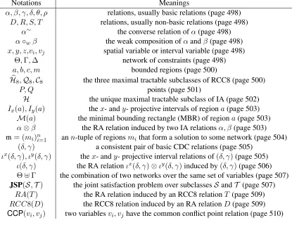
In both interpretations, the relations in Table 2 and the converses of TPP andNTPPform a JEPD set. Write Brcc8 andBrcc8′ for these two sets. We call the Boolean algebras generated by

Brcc8andBrcc8′, respectively, the weak and the strong RCC8 models, written as RCC8 and RCC8′. Strong connectedness has been considered by Borgo et al., (1996), Cohn and Varzi (1999), and Li et al., (2013). It is easy to see that, as relations, strong connectedness is contained in weak connectedness. Table 2 illustrates a configuration (the 2nd from the left) which is an instance ofEC

in RCC8 but an instance ofDCin RCC8′, and a configuration (the 2nd from the right) which is an instance ofTPPin RCC8 but an instance ofNTPPin RCC8′.

Relation Symb. Definition (weak) Definition (strong)

equals EQ a=b a=b

disconnected DC a∩b=∅ dim(a∩b)≤0

externally connected EC a∩b6=∅ ∧ a◦∩b◦ =∅ dim(a∩b) = 1

partially overlap PO a

◦_∩b◦ _6=∅∧ a6⊆b ∧ a6⊇b

a◦∩b◦ 6=∅∧

a6⊆b ∧ a6⊇b tangential proper part TPP a⊂b ∧ a6⊂b◦ a⊂b ∧ dim(∂a∩∂b) = 1

non-tangential proper part NTPP a⊂b◦ a⊂b∧ dim(∂a∩∂b)≤0

Table 2: The set of basic RCC8 and RCC8′_{relations, wherea, bare two plane regions andx}◦_,∂x,dim(x) denote, respectively, the interior, boundary, and dimension ofx. Note that for notational conve-nience we setdim(∅) =−1.

Remark 1. As far as consistency and realisations are concerned, Li (2006b) has shown that any consistent RCC8 network has a solution in any RCC model. The cubic realisation algorithm de-scribed there can be used to construct a solution in both the weak and the strong RCC8 models. This implies in particular that an RCC8 network has a solution in the weak RCC8 model iff it has a solution in the strong RCC8 model. As we will show in this paper, this is, however, not the case when cardinal directions are combined with topological relations.

In the following, we recall some important properties of the three maximal tractable subclasses b

H8,C8, andQ8of RCC8 identified by Renz (1999). A complete list of relations in these subclasses

can be found in Appendix A of the work of Renz (2002).

Lemma 2. SupposeRis a non-basic RCC8 relation such thatR∩ {DC,EC,PO}=∅. Then (1) R∈ Q8iffRis either{TPP,NTPP}or{TPP∼,NTPP∼}.

(2) R∈Hb8iffRis inQ8or one of the following relations

{TPP,EQ},{TPP,NTPP,EQ},{TPP∼,EQ},{TPP∼,NTPP∼,EQ}.

(3) R∈ C8iffRis inHb8, or either{NTPP,EQ}or{NTPP∼,EQ}.

We note the above lemma does not define these subclasses. In particular, these subclasses do include RCC8 relationsRsuch thatR∩ {DC,EC,PO} 6=∅.

Theorem 3(Renz, 1999). A consistent scenarioΘs of a path-consistent networkΘof constraints overHb8,C8, or overQ8can be computed inO(n2)time, by replacing every constraint(viRvj)∈Θ with(vibase(R)vj)∈Θs, wherebase(R)is a basic relation obtained as follows:

(1) IfR∈ B, thenbase(R) =R;

(2) else if{DC} ⊆R, thenbase(R) ={DC};

(3) else if{EC} ⊆RandS =Q8 orS =Hb8, thenbase(R) ={EC}; (4) else if{PO} ⊆R, thenbase(R) ={PO};

(5) else if{NTPP} ⊆RandS=C8, thenbase(R) ={NTPP}; (6) else if{TPP} ⊆R, thenbase(R) ={TPP};

(7) elsebase(R) =base(R∼_).

In what follows, we callΘsthecanonical consistent scenarioofΘ. 2.2.1 REALISATION OFBASICRCC8 NETWORKS

It is known that, for basic RCC8 networks, path-consistency implies consistency (Nebel, 1995). We next give a a short description of the cubic realisation algorithm proposed by Li (2006b), as we need to devise a similar algorithm later for the combination cases.

Given a basic RCC8 networkΘ ={viθijvj}ni,j=1, supposeΘis path-consistent. Anntpp-chain

inΘis defined to be a series of variablesvi1, vi2,· · · , vik such thatvisNTPPvis+1 ∈ Θfor all

s= 1,· · · , k−1. Thentpp-levell(i)of a variablevi is defined to be the maximum length of the ntpp-chains contained inΘthat ends withvi.

A realisation can be constructed as follows, where a variable may be interpreted as a bounded region with multiple pieces. Without loss of generality, we assume (viEQvj) ∈ Θonly when i =j. We first define for each variablevi a finite setXi ofcontrol pointsas follows. For eachi, introduce a pointPi tovi; ifviECvj orviPOvj, then introduce a pointPij tovi; ifviTPPvj or viNTPPvj, then put allXi points intoXj. We then expand each pointP inXi a little to obtain a squares(P). These squares are pairwise disjoint. Then, taking the union of these squares, we obtain an instantiation of bounded regions to thesevi. This works for all but theECandNTPPconstraints. Further modifications are needed to cope with these constraints (cf. Li, 2006b or Appendix C of this paper).

2.3 Interval Algebra and Rectangle Algebra

In this subsection, we recallInterval Algebra(IA) (Allen, 1983) andRectangle Algebra(RA) (Bal-biani et al., 1999). IA is the qualitative calculus generated by the 13 basic relations between closed intervals on the real line shown in Table 3. We write

Bint={b,m,o,s,d,f,eq,fi,di,si,oi,mi,bi} (3) for the set of basic IA relations. Ligozat (1994) defines thedimension2of a basic interval relation as 2 minus the number of equalities appearing in the definition of the relation (see Table 3). That is,

for basic relations we have

dim(eq) = 0,dim(m) = dim(s) = dim(f) = 1,dim(b) = dim(o) = dim(d) = 2. (4) For a non-basic relationRwe define

dim(R) = max{dim(θ) :θis a basic relation inR}. (5)

Relation Symb. Conv. Dim. Definition

before b bi 2 x+< y−

meets m mi 1 x+=y−

overlaps o oi 2 x−_{< y}−_{< x}+_{< y}+

starts s si 1 x−=y−< x+< y+ during d di 2 y− < x−< x+< y+ finishes f fi 1 y− _{< x}−_{< x}+_=y+

equals eq eq 0 x−=y−< x+=y+

(i) (ii)

Table 3: IA basic relations (i) definitions and (ii) conceptual neighbourhood graph, where x = [x−, x+], y = [y−, y+]are two intervals.

Nebel and B¨urckert (1995) have shown that there is a unique maximal tractable subclass of IA which contains all basic relations. This subclass, written asH, is known as the ORD-Horn class. Using the conceptual neighbourhood graph (CNG) of IA (Freksa, 1992), Ligozat (1994) gives a geometrical characterisation for ORD-Horn relations. Consider the CNG of IA (shown in Table 3 (ii)) as a partially ordered set(Bint,)(by interpreting any relation smaller than its right or upper neighbours). Forθ₁, θ₂∈ Bintwithθ1θ2, we write[θ1, θ2]as the set of basic interval relationsθ

such thatθ1 θθ2, and call such a relation aconvexinterval relation. An IA relationRis called pre-convexif it can be obtained from a convex relation by removing one or more basic relations with dimension lower thanR. For example,[o,eq] ={o,s,fi,eq}is a convex relation and{o,eq}is a pre-convex relation. Ligozat has shown that ORD-Horn relations are precisely pre-convex relations. Nebel and B¨urckert also show that every path-consistent IA network overHis consistent. Fur-thermore, we can construct a consistent scenario for every path-consistent IA network over Hin quadratic time.

SupposeRis an IA relation and let

Rcore={θ∈ Bint: dim(θ) = dim(R), θ∈R}. (6) By (6) it is clear thatRcore = {eq} iffR = {eq}, and Rcore = R∩ {b,o,d,di,oi,bi}if R∩ {b,o,d,di,oi,bi}is nonempty, andRcore_{=R\ {eq}otherwise. Then we have}

From Table 3 (ii) it is easy to see that a pre-convex relationRhas dimension 1 iff eitherRis a 1-dim basic relation orRis contained in{s,eq,si}or{fi,eq,f}. As a consequence, we know

Corollary 5. SupposeΘ = {viRijvj}ni,j=1 is a path-consistent network over H. ThenΘhas a consistent scenarioΘ∗_={v

iR∗ijvj}ni,j=1which has the following property: dim(R∗_ij) = dim(Rij), and

R∗

ij ={eq}only ifRij ={eq},R∗ij ={m}only ifRij ={m},R∗ij ={mi}only ifRij ={mi}. This result shows that, for any path-consistent networkΘoverH, we can construct in quadratic time a consistent scenario forΘ.

(i) (ii)

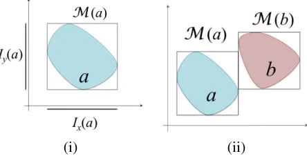
Figure 2: (i) The minimum bounding rectangleM(a)of a regiona; (ii) the RA relation ofatobis m⊗o.

IA can be naturally extended to regions in the plane. We assume an orthogonal basis in the Eu-clidean plane. For a bounded regiona, itsminimum bounding rectangle(MBR), denoted byM(a), is the smallest rectangle which contains aand whose sides are parallel to the axes of the basis. We writeIx(a)andIy(a)as, respectively, thex- andy-projections ofM(a). The basic rectangle relation between two bounded regionsa, bisα⊗βiff(Ix(a), Ix(b)) ∈αand(Iy(a), Iy(b))∈ β, whereα, β are two basic IA relations (see Figure 2 for illustration). We writeBrec for the set of basic rectangle relations, i.e.,

Brec ={α⊗β :α, β ∈ Bint}. (8)

There are 169 different basic rectangle relations inBrec. The Rectangle Algebra (RA) is the algebra generated by relations inBrec(Balbiani et al., 1999).

The following definitions will be used later.

Definition 6. Suppose α = ρ1 ⊗ρ2 is a basic RA relation. We say α is a 0-meet relation if ρ1, ρ2 ∈ {m,mi}, and is acornerrelation ifρ1, ρ2 ∈ {m,mi,s,si,f,fi,eq}. In general, we say a

non-basic RA relationR = {α₁, ..., αk}(k ≥ 2) is acornerrelation if eachαi (1 ≤ i≤ k) is a corner relation.

By definition, each 0-meet relation is a corner relation. Furthermore, it is easy to see that a basic RA relation α is a 0-meet relation iff, for every two rectanglesr, r′ with (r, r′) ∈ α, r∩r′ is a singleton in the plane; andαis a corner relation iff every two rectanglesr, r′ with(r, r′)∈αhave, at least, a corner point in common.

Lemma 7. Let∆ ={vi(Rij ⊗Sij)vj}ni,j=1be an RA network, whereRij andSij are arbitrary IA relations. Then∆is satisfiable iff its projections∆x _{= {x}

iRijxj}ni,j=1 and∆y ={yiSijyj}ni,j=1 are satisfiable IA networks.

By Corollary 5 and the above lemma we have

Lemma 8. Suppose∆ = {viRijvj}is a path-consistent RA network over H × H. Then∆has a consistent scenario∆∗_={v

iδijvj}such that

• δij is a 0-meet relation iffRij is a 0-meet basic relation, and

• δij is a corner relation iffRij consists only of basic corner relations.

As a consequence, we knowH ×His a tractable subclass of RA. No maximal tractable subclass has been identified for RA, but a larger tractable subclass of RA has been identified (Balbiani et al., 1999).

We next show that each path-consistent basic IA or RA network has a canonical solution in the following sense.

Definition 9(canonical tuple of intervals (rectangles)). Supposem= ([m−

i , m +

i ])ni=1is ann-tuple

of intervals. Let E(m)be the set of the values of the end points of intervals in m. We saymis

canonicaliff E(m) = {0,1,· · · , M}. A tuple of rectangles (m_i)n

i=1 is canonicaliff its x- and y-projections, (Ix(mi))n

i=1 and(Iy(mi))ni=1, are canonical tuples of intervals. A solution of an

IA (RA, respectively) network is called acanonicalsolution if it is a canonical tuple of intervals (rectangles, respectively).

For a basic satisfiable IA network, we can compute the total order of all the end points. Hence we can obtain a canonical solution (by assigning0to the first end point,1to the second, etc.). This gives us the following proposition.

Proposition 10. SupposeΘis a satisfiable basic IA (RA) constraint network. ThenΘhas a unique canonical solution.

2.4 Cardinal Direction Calculus

The cardinal direction calculus (CDC) was proposed by Goyal and Egenhofer (1997). Given a bounded regionbin the real plane, by extending the four edges ofM(b), we partition the plane into ninetiles, denoted bybij (1≤i, j≤3), see Figure 3 (i) for illustration.

For a primary region aand a reference region b, the CDC relation ofa tob, denoted byδab, is encoded in a3×3Boolean matrix (dij)1≤i,j≤3, wheredij = 1 iffa◦ ∩bij 6= ∅(wherea◦ is

again the interior of a). For example, the basic CDC relations δab andδba for the regionsa, bin Figure 3(ii) are represented by the following matrices.

δ∗=δab=

 

0 0 0 1 0 0 0 0 0



, γ∗=δba=

 

0 0 1 0 0 1 0 0 1



. (9)

(i) (ii) (iii)

Figure 3: Illustrations of (i) the nine tiles of a reference region; (ii) and (iii): two solutions of the CDC basic constraint network{v1δ∗v2, v2γ∗v1}, whereδ∗andγ∗are defined in Eq. (9).

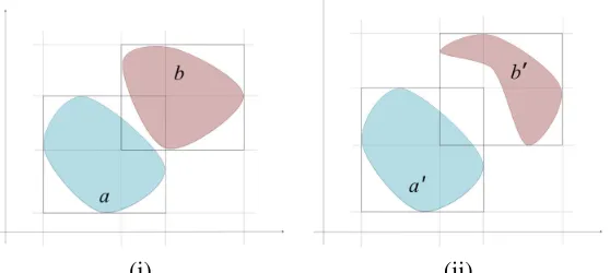
if the constraint network {v1δv2, v2γv1} has a solution. We also call γ a weak converseofδ if (δ, γ)is a consistent pair. Figure 4 shows that a basic CDC relation may have more than one weak converse. Therefore, we need both the relation ofatoband the relation ofbtoato give a complete description (in terms of the CDC calculus) of the directional information between two regionsa, b.

(i) (ii)

Figure 4: Illustration of two consistent CDC pairs (i)(δab, δba) and (ii)(δa′_b′, δ_b′_a), whereδ_ab = δa′_b′ butδ_ba =6 δ_b′_a′. Also note that the rectangle relation betweena, band that between a′, b′are botho⊗o.

In the following we show that there is a strong connection between CDC and RA relations.

Definition 11. (Zhang et al., 2008; Liu et al., 2010) For a pair of basic CDC relations(δ, γ), we define thex-projective interval relationof(δ, γ), written asιx(δ, γ), as the disjunction of all basic IA relationsαwhich has an instance that is the x-projection of some solution of{v1δv2, v2γv1},

i.e.

ιx(δ, γ) ={α∈ Bint: (∃m1, m2)[(m1, m2)∈δ ∧ (m2, m1)∈γ ∧ (Ix(m1), Ix(m2))∈α]}.

A similar definition applies for they-direction.

relation is an IA relationRwhich has the following property

R={b,m}orR={bi,mi}, orRis a basic IA relation in{o,s,d,f,eq,oi,si,di,fi}. (10) The two projective interval relations can then be combined into an RA relation.

Definition 12. (Zhang et al., 2008; Liu et al., 2010) For a pair of basic CDC relations(δ, γ), we callι(δ, γ) = ιx(δ, γ)⊗ιy(δ, γ)the RA relation inducedby (δ, γ). In general, for a basic CDC constraint network∆ ={viδijvj}ni,j=1, we callι(∆) = {viRijvj}ni,j=1the RA constraint network inducedby∆, whereRij =ι(δij, δji).

Note thatι(δ, γ)is not necessarily a basic RA relation. If(δ, γ)is consistent, then we know the RA relationι(δ, γ)has the formα⊗β, whereα, β are IA relations that satisfy (10). Furthermore, a solution of {v₁δv₂, v₂γv₁} is always a solution of {v₁ι(δ, γ)v₂}. We note that a solution of

{v1ι(δ, γ)v2}is not necessarily a solution of{v1δv2, v2γv1}.

Take the consistent pair (δ∗, γ∗)defined in (9) as an example. Figure 3 (ii) and (iii) show two solutions (a, b) and(a′_{, b}′_{) of the basic CDC constraint network {v}

1δ∗v2, v2γ∗v1}. This implies

by definition thatιx(δ∗, γ∗) contains{b,m}. It is easy to see from the definition that ιx(δ∗, γ∗)

contains no other basic IA relations andιx(δ∗, γ∗) ={b,m}. Similarly, we can showιy(δ∗, γ∗) =

{d}. This shows that this consistent pair(δ∗_{, γ}∗_{)corresponds to basic RA relations, viz.m⊗dand} b⊗d.

2.4.1 CANONICALSOLUTIONS OFBASICCDC NETWORKS

Just like IA and RA, consistent CDC networks also have ‘canonical’ solutions.

Definition 13 (regular solution, Zhang et al., 2008; Liu et al., 2010). Suppose m = (m_i)n

i=1 is

a solution of a basic CDC constraint network ∆. We say thatm ismaximal if m′

i ⊆ mi holds for any solution(m′_i)n

i=1 of∆withM(mi) = M(m′i); we saymisregularifmis maximal and (M(mi))ni=1is a canonical tuple of rectangles.

A basic CDC network in general has many regular solutions, but we have the following result.

Proposition 14. Let ∆be a basic CDC network. Suppose Γ is a basic RA network that refines ι(∆), the induced RA network of∆. Then we can determine in cubic time whether∆has a solution that also satisfiesΓ. Moreover, if∆has a solution, then it has auniqueregular solution which also satisfiesΓ. Furthermore, this unique regular solution can be constructed in cubic time.

Proof. The proof is similar to that for Proposition 12 in the work of Liu et al., (2010). A sketch is given in Appendix A.

From the proof of the above result, we can see that each regionmiin a regular solution(mi)ni=1

consists ofunit cells(i.e. rectangles of the form[i, i+1]×[j, j+1], wherei, j∈Z) in the canonical solution ofΓ, i.e. for each regionmiand each cellc, we have eitherc⊆mi orc∩mi◦ =∅.

For a basic CDC network∆, there may existexponentially manydifferent basic RA networks that refine ι(∆). Hence, ∆ may have exponentially many different regular solutions (see Fig-ure 11(a) for an example of such a network). However, to verify that∆has a solution, we need only prove that∆has a solution for somespecial basic RA network that refines ι(∆) (Liu et al., 2010, Proposition 12).3 Therefore, the consistency of∆can be determined in cubic time, and, if∆

is consistent, a regular solution can be constructed in cubic time (Liu et al., 2010).

3. The Joint Satisfaction Problem

After the preparatory introduction of basic notions and essential results of qualitative calculi, we are now ready to describe the joint satisfaction problem.

LetM1andM2be two qualitative calculi over the same domainU. SupposeSiis a subclass of Mi(i= 1,2). We writeJSP(S1,S2)for thejoint satisfaction problem(Gerevini & Renz, 2002; Li,

2007) overS1andS2.

Suppose Θ = {viTijvj}ni,j=1 is a constraint network overS1, and ∆ = {viDijvj}ni,j=1 is a

constraint network over S2 involving the same variables. Then we sayΘ⊎∆is an instance of

JSP(S1,S2). The joint satisfaction problem was first considered for RCC8 and the qualitative size

calculus (identical to the Point Algebra in Vilain & Kautz, 1986) by Gerevini and Renz (2002). Moreover, it was shown that the consistency of a joint network can be approximated by the poly-nomial bipath-consistency algorithm. Li and Cohn (2012) recently showed that bipath-consistency can be equivalently expressed as below.

Definition 15. LetΘ⊎∆be a joint constraint network overM1andM2, whereΘ ={viTijvj}ni,j=1

and∆ ={viDijvj}ni,j=1. We sayΘ⊎∆isbi-closedifα∩Dij andTij ∩βare nonempty for any basic relationα ∈ Tij, any basic relationβ ∈ Dij, and any1 ≤ i, j ≤ n (here we regard each relation as a subset ofU×U). A bi-closed joint networkΘ⊎∆isbipath-consistentifΘand∆are both path-consistent.

Informally speaking, a joint constraint network is bi-closed if each basic relation of a given relation in one of the calculi is consistent with the corresponding relation in the other calculus.

As a simple example of the joint satisfaction problem, we consider the combination of RA and CDC in the next subsection.

3.1 The Combination of RA and CDC

Let R be a basic CDC relation. Then R∼, the set-theoretic converse (or inverse) relation of R (cf. (1)), may be not representable in the relation algebra CDC (Cicerone & Di Felice, 2004; Liu et al., 2010). That is,R∼cannot be represented as the union of several basic CDC relations. In this sense, we say the CDC isnotclosed under converse. Recently, Schneider et al. (2012) proposed a variant of CDC, called the Object Interaction Model (OIM), which is closed under converse.

For two bounded regions a, b, OIM divides the plane into up to(l1 + 2)×(l2 + 2) tiles by

extending the edges of M(a) andM(b), wherel1 + 1 andl2+ 1 are the numbers of horizontal

and, respectively, vertical lines. It is clear that1≤l₁, l₂ ≤3since edges ofM(a)andM(b)may coincide. The OIM relationφabis represented by anl1×l2matrix (also written asφab) considering existence of interior points ofaand/orbin corresponding bounded tiles. Let T be such a bounded tile. We set the entry corresponding to T in the matrixφabto 0 if T has no interior point which is in eitheraorb; and set it 1 (2, respectively) if T has an interior point which is ina(b, respectively) and has no interior point which is inb(a, respectively); and set it 3 otherwise. The converse relation of a basic OIM relation is also a basic OIM relation. In particular, the basic OIM relationφbaofbtoa can be obtained by swapping the occurrences of 1 and 2 inφab.

For example, the OIM relations between the regions in Figure 3 (ii) and (iii) are respectively

φab =

 

0 0 2 1 0 2 0 0 2



, φa′_b′ =

 

0 2 1 2 0 2

and the OIM relations between the regions in Figure 4 are respectively

φab=

 

0 2 2 1 3 2 1 1 0



, φa′_b′ =

 

0 2 2 1 1 2 1 1 0

 .

We note that for regionsa, b, a′, b′ in both figures we haveδab = δa′_b′. This suggests that OIM is finer grained than CDC in the sense that it splits one basic CDC relation into several OIM relations. Nevertheless, since CDC is not closed under converse, we need to consider consistent pairs of basic CDC relations in order to evaluate its expressivity. When comparing the expressivity of the two calculi in this way, we can see that(δab, δba)6= (δa′_b′, δ_b′_a′)in Figure 4, but(δ_ab, δ_ba) = (δ_a′_b′, δ_b′_a′) in Figure 3. This shows that OIM makes finer distinctions than CDC in describing the scenarios given in Figure 3(ii) and (iii): when sayingais westofb, CDC does not differentiate if the east boundary ofameets or precedes the west boundary ofb. The following result shows that OIM is only finer than CDC in describing these cardinal relations, and it is in essence the combination of CDC and RA.

Theorem 16. (Li & Liu, 2014) For any two regionsaandb, we can compute the RA relation ofa tob, the CDC relation ofatob, and the CDC relation ofbtoafrom the OIM relation ofatob, and vice versa.

In other words, for each basic OIM relation θ, there exist two basic CDC relationsδ, δ′ and a basic RA relationγsuch thatθ=δ∩δ′∼∩γ, i.e. for any two regionsaandb, the relationθis the OIM relation ofatobiffδ,δ′andγare, respectively, the CDC relation ofatob, the CDC relation ofbtoa, and the RA relation ofatob. Because basic CDC and RA relations are both JEPD, the above choices ofδ, δ′, γare unique. In the following, we callδthe CDC relation induced byθand callγ the RA relation induced by θ. Note that in this caseδ′ (as a relation ofbtoa) is the CDC relation induced byθ∼, which is the OIM relation ofbtoa.

As a consequence, we have the following result.

Proposition 17. SupposeΘ = {viθijvj}n

i,j=1 is a basic OIM network such thatθji=θij∼for any i, j. Let∆ ={viδijvj}ni,j=1andΓ = {viγijvj}ni,j=1, whereδij andγij are, respectively, the CDC relation and the RA relation induced by θij. ThenΘ is consistent iff the joint network∆⊎Γ is consistent.

Proof. Recall that the converse of a basic OIM relation is also a basic OIM relation. Because θji=θij∼, it is straightforward to show that θij =δij ∩δ∼ji∩γij. Therefore, solutions of Θ are exactly the solutions of∆⊎Γ.

As a consequence of Propositions 14 and 17 we have

Corollary 18. LetΘ,∆andΓbe as given in Proposition 17. ThenΓis a basic RA network that refinesι(∆), and the consistency ofΘcan be determined in cubic time. Moreover, ifΘis consistent, then there is a unique regular solution of∆that is also a solution ofΘ.

4. Combination of Weak RCC8 and RA Networks

In this section we represent topological information as weak RCC8 relations and directional infor-mation as RA relations. We first consider the interaction between weak RCC8 and RA relations, then consider the JSP for basic constraints, and, lastly, consider the JSP in general.

4.1 Interaction Between Weak RCC8 and RA Relations

Relations in different calculi may interact in the sense that a relation from one calculus may intersect with several relations from the second calculus. We here recall related definitions and preliminary results obtained by Li and Cohn (2012).

Definition 19. LetT be an RCC8 relation andDan RA relation. The RA relation induced byT and the RCC8 relation induced byDare defined as

RA(T) ={δ :δis a basic RA relation andδ∩T 6=∅} (11) RCC8(D) ={θ:θis a basic RCC8 relation andθ∩D6=∅}. (12) Note that a joint networkΘ⊎∆isbi-closedifδij ⊆RA(θij)andθij ⊆RCC8(δij)for anyi, j.

It is easy to see (cf. Li and Cohn, 2012) thatRA(T) =S{RA({θ}) :θ∈T}and

RA({DC})⊃RA({EC})⊃RA({PO})⊃RA({TPP})⊃RA({NTPP,EQ}), (13) RA({PO})⊃RA({TPP∼})⊃RA({NTPP∼,EQ}), (14) where, for example,RA({EC}) ⊃RA({PO})holds because, for each basic RA relationδ,δ is inRA({EC})ifM(a)∩ M(b)6=∅for all(a, b)∈δ, andδis inRA({PO})ifM(a)∩ M(b)is a non-degenerate rectangle for all(a, b)∈δ.

Lemma 20. LetT be an RCC8 relation andDan RA relation. ThenRCC8(D)is a relation in the intersection ofHb8,Q8, andC8; andRA(T)is a relation inH × HifT is a relation inHb8orQ8. Proof. This follows from the definitions ofRCC8(D)andRA(T)and a simple table look-up from Appendix A of the work of Renz (2002).

The second statement does not apply to relations inC8. For example, considerT ={NTPP, EQ}. ThenTis a relation inC8, butRA(T) ={d⊗d,eq⊗eq}is outsideH × H.

4.2 Combination of Basic Networks

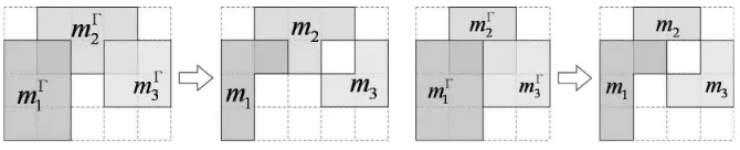
We now consider the combination of RCC8 and RA. First we show that bipath-consistency is not sufficient for consistency inJSP(Brcc8,Brec) (Li & Cohn, 2012). LetΓ = {viγijvj}4i,j=1 be the

basic RA network induced by the four rectanglesmΓ_i (i= 1,2,3,4)illustrated below.

LetΘ = {viθijvj}4_i,j=1 be the basic RCC8 constraint network in whichθ12 = θ34 = {EC}and

all the others are{DC}. Clearly,Θis satisfiable. Although Θ⊎Γ is bipath-consistent, it is not satisfiable. This is because, otherwise, there exists a solutionm= (m_i)4

i=1andM(m1)∩M(m2) =

M(m3)∩ M(m4) ={P}is a singleton. Byθ12=θ34={EC}we knowP ∈mi(i= 1,2,3,4).

This contradictsθ13={DC}.

Definition 21 (conflict point). LetΘ = {viθijvj}ni,j=1 be a basic RCC8 network and Γ = {vi γijvj}n

i,j=1a basic RA network. SupposemΓis the canonical solution ofΓ. A pointQis called a conflict pointofmΓ_i if there existsjsuch thatmΓ_i ∩mΓ_j ={Q}andθij ={EC}. We writeCifor the set of all conflict points ofmΓ_i.

Clearly, each conflict point ofmΓ_i is also a corner point ofmΓ_i. This implies thatmΓ_i andmΓ_j may have at most one common conflict point. Moreover, suppose m = (m_i)n

i=1 is a solution of Θ⊎Γsuch thatM(mi) =miΓ for all1 ≤i ≤n. Then each conflict point ofmΓi is contained in mi. This meansCi ⊂mi. As a consequence, we have

Ci∩Cj 6=∅⇒θij 6={DC} (1≤i, j≤n) (15) The following theorem shows that this is also sufficient.

Theorem 22. LetΘ ={viθijvj}ni,j=1be a basic RCC8 network andΓ ={viγijvj}ni,j=1a basic RA network. SupposeΘ⊎Γis bipath-consistent. ThenΘ⊎Γis satisfiable iff (15)holds.

Proof. The necessity part is clear. We defer the proof of the sufficiency part to Appendix B.

As a corollary, we haveJSP(Brcc8,Brec)is in P.

Corollary 23. For a basic RCC8 networkΘand a basic RA networkΓ, the consistency ofΘ⊎Γ can be decided in cubic time.

Proof. Bipath-consistency of Θ⊎Γcan be checked in cubic time. We can construct the unique canonical rectangle solution ofΓin quadratic time. The conflict point setCican also be computed in quadratic time. That is, the condition of Theorem 22 can be checked in cubic time.

4.3 Large Tractable Subsets

Recall that RCC8 has three maximal tractable subclassesHb8,C8, andQ8, and IA has one maximal

tractable subclassH, all containing the basic relations. In this subsection, we aim to extend the above result to maximal tractable subsetsHb8,C8of RCC8, and the large tractable subsetH × Hof

RA.

To this end, we need to extend the notion of conflict points from basic networks to arbitrary networks. Recall that 0-meet relations and corner relations are basic RA relations defined in Defi-nition 6.

Definition 24(common conflict point). LetΘ = {viTijvj}ni,j=1 be an RCC8 network and ∆ =

{viDijvj}ni,j=1an RA network. We say two variablesvi, vj have the CCP (common conflict point) relation, writtenCCP(vi, vj), ifDij is a 0-meet (basic) relation andTij ={EC}, or

• there existi′, j′ such thatDii′ andD_jj′ are 0-meet (basic) relations,D_ij′, D_i′_j andD_i′_j′ are (possibly disjunctive) corner relations, andTii′ =T_jj′ ={EC}.

IfCCP(vi, vj) andvi′, vj′ are variables that satisfy the above conditions, we also writeCCP(i, j : i′, j′)to stress the roles ofvi′ andv_j′.

(i) (ii)

Figure 5: Two joint constraint networks in JSP(RCC8, RA), where in both (i) and (ii) Dij is the basic RA relation between vi and vj as illustrated in the pic-ture, T14 = T23 = {EC} and all unspecified RCC8 constraints are

non-basic RCC8 relation {DC,EC,PO}. In both (i) and (ii) we have CCP(1,2),CCP(1,3),CCP(1,4),CCP(2,3),CCP(2,4),CCP(3,4).

Examples are shown in Figure 5. Note that ifΘand∆are all basic networks, then vi andvj have the CCP relation iffCi∩Cj is nonempty, i.e.viandvj have a common conflict point.

Definition 25. Let Θ = {viTijvj}ni,j=1 be an RCC8 network and∆ = {viDijvj}ni,j=1 an RA

network. We sayΘ⊎∆isCCP-consistentif

CCP(vi, vj)⇒DC6∈Tij (16) holds for anyi 6= j. We say a joint networkΘ⊎∆isBC-consistentif it is bipath-consistent and CCP-consistent.

In general, if vi andvj have the CCP relation, then (in any realisation)vi andvj share at least one corner point (of their MBRs) in common. Therefore, in the weak RCC8 algebra, they cannot be disconnected, and neither can be contained in another as a non-tangential proper part. Note that the latter statement also follows from the bi-closedness ofΘ⊎∆.

Similar to the bipath-consistency algorithm (Gerevini & Renz, 2002), we devise an algorithm (Algorithm 1) for enforcing BC-consistency. The following theorem shows that this algorithm is sound.

Theorem 26. SupposeΘ⊎∆is a joint network of RCC8 and RA constraints, whereΘ = {viTij vj}n

Input: A joint networkΘ⊎∆, whereΘ ={viTijvj}i,jn =1and∆ ={viDijvj}ni,j=1.

Output: false, if an empty constraint is generated; a BC-consistent joint network equivalent toΘ⊎∆, otherwise.

Q← {(i, k, j)|i6=j, k6=i, k6=j}; (iindicates thei-th variable ofΘ⊎∆. Analogously forjandk)

whileQ6=∅do

select and delete a path(i, k, j)fromQ;

ifBC-REVISION(i, k, j)then

ifTij =∅orDij =∅then returnfalse;

end

Q←Q∪ {(i, j, k),(k, i, j)|k6=i, k 6=j};

end end

Function: BC-REVISION(i, k, j)

Input: three variablesi, kandj

Output: true, ifTij orDij is revised; false otherwise.

Side effects:Tij andDjirevised using the operations∩and◦w. Tij ←

(Tij∩RCC8(Dij))∩(Tji∩RCC8(Dji))∼∩(Tik∩RCC8(Dik))◦w(Tkj∩RCC8(Dkj)); Dij ←(Dij ∩RA(Tij))∩(Dji∩RA(Tji))∼∩(Dik∩RA(Tik))◦w(Dkj∩RA(Tkj));

ifCCP(i, j :k)then

Tij ←Tij \ {DC};

end

ifneitherTijnorDij is revisedthen

returnfalse;

end

Dji←D∼ij; Tji←T_ij∼;

returntrue.

Proof. This is because, if we iteratively use the following updating rules then either an empty con-straint occurs or the network becomes stable.

Tij ←(Tij ∩RCC8(Dij))∩(Tji∩RCC8(Dji))∼

∩(Tik∩RCC8(Dik))◦w(Tkj∩RCC8(Dkj)) (17) Dij ←(Dij ∩RA(Tij))∩(Dji∩RA(Tji))∼∩(Dik∩RA(Tik))◦w(Dkj ∩RA(Tkj)) (18) Tij ←Tij \ {DC}ifCCP(i, j:k), (19) wherei, j, krepresent the variablesvi, vj andvk andCCP(i, j :k)represents the situation where there exists another variablevl such thatvl andvk together are evidence of CCP(i, j). For each triple,CCP(i, j :k)can be determined inO(n)time and the subroutine BC-REVISION(i, k, j) can

be carried out inO(n)time. Since eachTij is a set of basic RCC8 relations and eachDij is a set of basic RA relations,(Tij, Dij)can be revised for a constant number of times. Therefore the number of the loops remains cubic, and BC-CONSISTENCYwill terminate inO(n4)time.

The algorithm is in general not complete. The following lemma will be useful to prove the main result (Theorem 28), which will guarantee the completeness of the algorithm for RCC8 networks overHb8 and RA networks overH × H.

Lemma 27. LetΘ ={viTijvj}ni,j=1be an RCC8 network and∆ ={viDijvj}ni,j=1an RA network. SupposeΘ is overHb8 or Q8 andΘ⊎∆ is bipath-consistent. Assume that Θ∗ is the canonical consistent scenario ofΘ(cf. Theorem 3), and∆∗_{is any consistent scenario of∆. ThenΘ}∗_⊎∆∗_is bipath-consistent.

Proof. Because bothΘ∗_and∆∗_{are path-consistent basic networks, we need only show thatΘ}∗_⊎∆∗ is bi-closed, i.e.δ∗_ij ∈RA(θ_ij∗)andθ_ij∗ ∈RCC8(δ_ij∗)for anyi6=j. Sinceθ_ij∗ andδ_ij∗ are both basic relations, this is equivalent to showing thatθ∗_ij ∩δ∗_ij is nonempty for anyi6=j. By (13) and (14) it is straightforward to show thatRA(Tij) =RA(θ∗ij). Thereforeδ∗ij ⊆Dij ⊆RA(Tij) =RA(θ∗ij), i.e.δ_ij∗ ∩θ_ij∗ is nonempty.

We note that this result does not apply to C8. For example, let T = {NTPP,EQ}, D =

{d⊗d,eq⊗eq}. The RCC8 relationNTPPis inconsistent with the RA relationeq⊗eq.

Theorem 28. LetΘ ={viTijvj}ni,j=1 be an RCC8 network and∆ = {viDijvj}ni,j=1 an RA net-work. SupposeΘis overHb8, and∆is overH × H. ThenΘ⊎∆is consistent if it is BC-consistent. Proof. Recall that each RA network overH × His in essence a pair of IA networks overH. By Lemma 8 we know∆has a consistent scenario∆∗ _{such that (i)δ}∗

ij is a 0-meet relation iffDij is; and (ii)δ∗_ijis a corner relation iffDijconsists of corner relations. LetΘ∗be the canonical consistent scenario ofΘ. We showΘ∗_⊎∆∗_{is consistent.}

By Lemma 27 we knowΘ∗_⊎∆∗_{is bipath-consistent. We next show it satisfies (15), which is} equivalent to (16) when only basic constraints are concerned. To this end, we show thatCCP(i, j: i′_{, j}′_{)holds inΘ}∗ _⊎∆∗ _{only if it holds in Θ⊎∆. By the choice of∆}∗ _andΘ∗_{, we knowT}

As a consequence, we know the joint consistency problem overHb8 orQ8 andH × Hcan be

solved in polynomial time.

Theorem 29. The joint satisfaction problemsJSP(Hb8,H × H)andJSP(Q8,H × H)are in P. Proof. Suppose Θ⊎∆is a joint network such thatΘis overHb8 orQ8, and∆is over H × H.

We first apply the algorithm BC-CONSISTENCYtoΘ⊎∆. If an empty relation occurs during the process, thenΘ⊎∆is inconsistent. Otherwise, supposeΘ′_⊎∆′_{is the BC-consistent joint network} equivalent toΘ⊎∆. We assert thatΘ′_{is still overHb}

8 orQ8and∆′is overH × H. We note that,

for any RCC8 relationT inHb8(orQ8), and any RA relationDinH × H, we have by Lemma 31

• RCC8(D)is a relation in bothHb8 andQ8;

• RA(T)is a relation inH × H;

• T\ {DC}=T ∩ {EC,PO,TPP,NTPP,TPP∼,NTPP∼,EQ}is inHb8(orQ8).

Because BC-CONSISTENCYonly uses the rules (17)-(19) to update relations, each RCC8 relation inΘ′remains inHb8(orQ8), and each RA relation in∆′remains inH×H. The consistencyΘ′⊎∆′

then follows from Theorem 28.

The property in the proof of the above theorem does not hold for C8. It remains open if

JSP(C8,H × H)is tractable (though this is not very important for practical purposes since either

b

H8orQ8can be used to backtrack over to find a solution if required).

5. Combination of RCC8′ and RA Networks

In this section, we represent topological information as RCC8′relations and directional information as RA relations. In the previous section we have shown that, for certain tractable subclasses of RCC8 and RA, the JSP can be determined in polynomial time, but we also show that bipath-consistency is incomplete for these subclasses. The reason lies in that two regions that are constrained byDC

may have a common conflict point. For RCC8′, this situation does not exist anymore because two disjoint regions may still have a 0-dimensional intersection. This section will show that, for RCC8′, bipath-consistency alone is sufficient to show the consistency of a joint networkΘ⊎∆forΘover

H8orC8 and∆overH × H.

As in the case of weak RCC8, we first consider the interaction between RCC8′and RA relations, then consider the consistency of joint basic networks, and, lastly, consider the general case.

Similar to Definition 19, we have the following definition.

Definition 30. LetT be an RCC8′ relation andDan RA relation. The RA relation induced byT and the RCC8′relation induced byDare defined as

RA(T) ={δ :δis a basic RA relation andδ∩T 6=∅} (20) RCC8′(D) ={δ :θis a basic RCC8′ relation andθ∩D6=∅}. (21) It is easy to see thatRA(T) =S{RA({θ}) :θ∈T}and

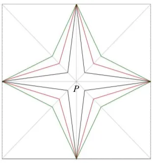
Note that we haveRA({TPP}) =RA({NTPP})={s,d,f,eq} ⊗ {s,d,f,eq}. This is because in RCC8′ a non-tangential proper part of a regionamay have the same MBR asa. For example, each star region in Figure 6 is a non-tangential proper part of its MBR in RCC8′.

Lemma 31. LetT be an RCC8′ relation andDan RA relation. ThenRCC8′_{(D)is a relation in} the intersection ofHb8,Q8, andC8; andRA(T)is a relation inH × HifT is a relation inHb8or

Q8 orC8.

In particular, unlike the case for weak RCC8, we haveRA({NTPP,EQ}) ={s,d,f,eq} ⊗ {s,d,f,eq}is a relation inH × H.

Figure 6:Basic regions of a control pointPin the combination of RCC8′_{and RA.}

Theorem 32. SupposeΘis a basic RCC8′ network and∆is a basic RA network. ThenΘ⊎∆is consistent if it is bipath-consistent.

Proof. The proof follows the same pattern as for the combination of weak RCC8 and RA (The-orem 22), but we need to replace the basic regions around a control point P with the star re-gions shown in Figure 6, where we only show three rere-gions b, r, g aroundP, and bNTPPr and rNTPPg.

We have the following result for RCC8′ and RA.

Theorem 33. SupposeΘis a network overHb8 orQ8in RCC8′,∆is an RA network. ThenΘ⊎∆ is consistent ifΘ⊎∆is bi-closed,Θis path-consistent, and∆is consistent.

Proof. Assume thatΘ∗_{is the canonical consistent scenario ofΘ, and∆}∗_{is any consistent scenario} of∆. Then, completely similar to Lemma 27, we can show thatRA(θ∗_ij) =RA(θij)and hence the bi-closeness ofΘ∗_⊎∆∗_{. BecauseΘ}∗_and∆∗_{are consistent, we knowΘ}∗_⊎∆∗_{is bipath-consistent,} hence consistent by Theorem 32.

The above result shows that the consistency of a joint network inJSP(Hb8, RA)can be

polyno-mially reduced to determining the consistency of an RCC8 network overHb8 and an RA network.

Theorem 34. If RCC8 relations are interpreted by using strong connectedness, then the joint satis-faction problemsJSP(Hb8,H × H)andJSP(Q8,H × H)are in P.

Again, it remains open whether the above result holds for networks over C8 in RCC8′, even

though in this caseRA({NTPP,EQ}) =RA(TPP)is a relation inH × H.

In the following section, we consider the combination of RCC8 and CDC constraints.

6. Combination of RCC8 and CDC Constraints

Although basic RCC8 networks and basic CDC networks can be solved in cubic time indepen-dently, the interaction between RCC8 and CDC constraints makes the joint satisfaction problem hard to solve. In this section, we first show that the joint satisfaction problem is in NP by de-signing a polynomial non-deterministic algorithm and then show it is NP-hard even for basic con-straints. This shows that JSP(Brcc8,Bcdc) is NP-complete. We then consider three variants of

JSP(Brcc8,Bcdc)obtained by replacing RCC8 with RCC8′and/or CDC with OIM. WriteBoimfor the set of basic OIM relations. We showJSP(Brcc8,Boim)andJSP(Brcc8′,B_cdc)are NP-complete, butJSP(Brcc8′,Boim)is in P.

6.1 Algorithms

LetΘbe an instance of a joint basic RCC8 or RCC8′ network and∆a basic CDC or OIM network over the same set of variables. We provide in this subsection algorithms for determining the consis-tency ofΘ⊎∆. Our key idea is first showing thatΘ⊎∆is consistent iff∆has a regular solution that is RA consistent withΘ(see below) and then giving algorithms for determining whether∆has such a regular solution.

Supposem= (m_i)n

i=1is a solution of∆. Recall that we saym= (mi)ni=1is aregular solution

if it is a maximal solution and{M(mi)}ni=1 is a canonical tuple of rectangles (cf. Dfn. 13). Note

that each region in a regular solutionmis the union of a set of cells introduced by the canonical

tuple of rectangles.

Definition 35. LetΘ = {viθijvj}ni,j=1 be a basic RCC8 network and∆ = {viδijvj}ni,j=1a basic

CDC network. Suppose m = (m_i)n

i=1 is a regular solution of∆. WriteΓ for the RA network

induced bym. We say a regular solutionmof∆isRA consistentwithΘif there exists a solution of

Θ⊎∆which also satisfiesΓ.

The following lemma gives a characterisation of consistent joint basic networks.

Lemma 36. LetΘ = {viθijvj}n

i,j=1 be a basic RCC8 network and∆ = {viδijvj}ni,j=1 a basic CDC network. ThenΘ⊎∆is consistent iff∆has a regular solution that is RA consistent withΘ. Proof. The sufficiency part is clear by definition. We only prove the necessity part. Supposea =

(ai)ni=1is a solution ofΘ⊎∆. WriteΓfor the RA network induced bya. Thenais also a solution of ∆⊎Γ. Hence there is a unique regular solution of∆which also satisfiesΓ. Writem= (mi)n

i=1for

this regular solution. It is clear thatmis a regular solution of∆that is RA consistent withΘ.

By this lemma, to determine the consistency of Θ⊎∆, we need only determine the existence of regular solutions of∆that are RA consistent withΘ. Supposemis a regular solution of∆. We

To this end, we first fix some notation and terminology. For a regionmi inm, we say a corner

pointP ofmi is apotential conflict point(in m) if exactly one of the four cells incident toP is

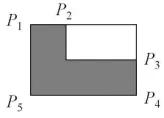
contained inmi. For example, the grey region shown in Figure 7 has five potential conflict points Pi(i= 1, ...,5). Later we will show that these points may introduce conflicts that are hard to resolve when RCC8 constraints are involved. Furthermore, we denote byGi the set of cells contained in mi,Eithe set of edges of cells which lie on the boundary ofmi, andNithe set of potential conflict points ofvi.

Figure 7: Illustration of potential conflict points.

Lemma 37. LetΘ = {viθijvj}n

i,j=1 be a basic RCC8 network and∆ = {viδijvj}ni,j=1 a basic CDC network. If a regular solutionm= (m_i)n

i=1of∆is RA consistent withΘ, then we have: ifθij =TPPorNTPPthenGi⊆Gj. (22)

Proof. We prove this by contradiction. Assume that(viTPPvj)or(viNTPPvj)is a constraint in

ΘandGi *Gj.

Suppose(vsδvt)is a constraint in∆, whereδis a basic CDC relation represented by the3×3 Boolean matrix(dpq)1≤p,q≤3. Becausemis a solution of∆, we have for any1≤p, q≤3that

dpq= 1 iff m◦_s∩mpq_t 6=∅, (23) wherempq_t denotes one of the nine tiles generated by the MBR ofmt(cf. Fig. 3). Sincemis a

regular solution andGsis the set of cells contained inms, this is equivalent to saying that

dpq= 1 iff Gsandmpqt have a common cell. (24) Now letg be a cell inGi \Gj. Becausegis not inGj, by the construction procedure of regular solutions (see Appendix A), there exists a constraint(vjδ′vk)∈∆withδ′ = (d′uv)such thatgis a cell contained inmpq_k for somep, q. By (24) and thatgis not inGj we knowd′pq = 0 and hence, by (23),m◦_j ∩mpq_k =∅. Let(viδ′′vk)be the CDC constraint betweenviandvkin∆and suppose δ′′_{= (d}′′uv_{). Becausegis cell in bothG}

iandmpq_k , we haved′′pq = 1by (24). Becausemis RA consistent with Θ, there exists a solution a = (ai)n

i=1 ofΘ⊎∆such that

M(ai) = M(mi). Since(viTPPvj)or(viNTPPvj) is inΘ, we knowai ⊂aj. Furthermore, we haveaj ⊆ mj asmis a maximal solution of∆. Therefore, a_i ⊂ m_j. Because mpq

k = a pq k andm◦_j ∩mpq_k = ∅,a◦_i ∩apq_k is empty. This shows that(ai, ak) is not inδ′′ sinced′′pq = 1. A contradiction.

TheNTPPconstraints may furthermore exclude some edges inEiand nodes inNi from the valuation ofvi. SupposeviNTPPvj is a constraint inΘandm= (m_i)n

i=1is RA consistent with Θ. For any solutiona= (ai)n_i

we haveaj ∩∂mj = ∅. This is to say,ai cannot touch the edges and nodes in Ej andNj. To characterise this, we define

¯

Ei ≡Ei\

[

{Ej :viNTPPvj ∈Θ}, (25) ¯

Ni ≡Ni\[{Nj :viNTPPvj ∈Θ}. (26) Since every region inmcan be represented by a Boolean matrix,G_i,E¯_i,N¯_i can be calculated

in polynomial time. The following proposition then gives a necessary and sufficient condition form

being RA consistent withΘ.

Lemma 38. LetΘ = {viθijvj}ni,j=1 be a basic RCC8 network and∆ = {viδijvj}ni,j=1 a basic CDC network. Then a regular solutionm= (mi)n_i

=1of∆is RA consistent withΘiff

• viTPPvj ∈ΘorviNTPPvj ∈ΘimpliesGi⊆Gj, and

• M(SE¯i) =M(mi)for anyi, and

• viPOvj ∈ΘimpliesGi∩Gj 6=∅, and

• there exists a resolving functionf, which is defined as a function fromV toP(S{N¯1,· · ·,Nn¯ }) satisfying(27)-(29).

f(vi)⊆N¯i, (27)

viECvj ∈Θ⇒Gi∩Gj 6=∅orE¯i∩E¯j 6=∅orf(vi)∩f(vj)6=∅, (28) viDCvj ∈Θ⇒f(vi)∩f(vj) =∅. (29)

Proof. We begin with the necessity part. Supposemis RA consistent withΘ. Then by definition

there exists a solutiona = (ai)n

i=1 ofΘ⊎∆such thatM(ai) = M(mi). The first condition is

proven in Lemma 37. For the second condition, becauseM(ai) =M(mi), andai⊆mi, we know thataihas a nonempty intersection with one unit edge on a cell that lies on the top (bottom, leftmost, or rightmost) edge ofM(mi). This unit edge is clearly inEi. Furthermore, it can be proven that this edge is inE¯i, and thus we haveM(SE¯i) =M(mi). The following two conditions guarantee that thePO,ECconstraints can be satisfied while not violatingDCconstraints. The third condition follows directly fromai⊆SGiandaiPOaj. For the last condition, we define a resolving function f asf(vi) ={P ∈N¯i :P ∈ai}. It is straightforward to prove thatf satisfies (27)-(29).

For the sufficiency part, we construct a solution ofΘ⊎∆. The procedure is quite similar to that given for Theorem 22 in Appendix B. Forvi, we choose a control point from each cell inGi and a control point from each edge inE¯i. IfviPOvj, we choose a control point for both of them from a common cell ofGi andGj. IfviECvj, we choose a control point for them in a common cell if Gi∩Gj 6= ∅, or from a common edge ifEi¯ ∩Ej¯ =6 ∅, or fromf(vi)∩f(vj) by the resolving functionf. It can then be proven that these control points lead to a solution of Θ. Moreover, the choice of control points ensures that the regions are also a solution of∆.

Since the conditions in Lemma 38 can be verified by a nondeterministic polynomial algorithm, we have the following theorem.