A novel algorithm for calculating transition potential in cellular automata models of land use/cover change

Contents lists available atScienceDirect

Environmental Modelling & Software

journal homepage:www.elsevier.com/locate/envsoft

A novel algorithm for calculating transition potential in cellular automata

models of land-use/cover change

Majid Shadman Roodposhti

_{, Jagannath Aryal}

_{, Brett A. Bryan}

a_{Discipline of Geography and Spatial Sciences, School of Technology, Environments and Design, University of Tasmania, Churchill Ave, Hobart, TAS, 7005, Australia} b_{Centre for Integrative Ecology, School of Life and Environmental Sciences, Deakin University, 221 Burwood Hwy, Burwood, VIC, 3125, Australia}

A R T I C L E I N F O

Keywords:

Entropy

Land-use/cover change Uncertainty Urban planning Modelling Simulation

A B S T R A C T

Despite recent advances in quantifying land-use/cover change (LUCC) transition potential, transition rules are often not transparent and uncertainty is rarely made explicit. Here, we introduce DoTRules—a dictionary of trusted rules—as a transparent alternative to calculate transition potential in cellular automata models. Rules relate LUCC variables to the observed historical changes. Shannon entropy is calculated to assess the uncertainty of each rule, and the most trusted rules are used to project future LUCC. DoTRules produces rule-level un-certainty estimates, which can be mapped. In a case study of the Ahvaz region of Iran, the overall accuracy of LUCC simulation calibrated using DoTRules was very similar to simulations calibrated with the state-of-the-art random forest, but DoTRules provides a more transparent approach where transition rule information and un-certainty can be readily accessed and interpreted. The results demonstrate that DoTRules has potential to derive new insights into LUCC processes.

1. Introduction

Cellular automata (CA) were conceptually established by John von Neumann (1903–1957) during the 1950s. Due to their simplicity and capacity to simulate spatial patterns, CA have rapidly gained popularity as a tool for modelling spatial dynamics of many environmental phe-nomena such as plant population dynamics (Xu et al., 2010), forest fire spread (Zheng et al., 2017), slope failure (Liucci et al., 2017), debris flow (D'Ambrosio et al., 2003;D'Ambrosio et al., 2006), urban sprawl (Mustafa et al., 2018a;Van Vliet et al., 2009), land-use/cover change (LUCC) (Hewitt and Díaz-Pacheco, 2017;Hewitt et al., 2014;White and Engelen, 1997) and more. Though cellular automata can handle very complex spatial situations for modelling environmental phenomena, their conceptual basis is straightforward. A cellular automaton consists of a large number of cells, which can change their state according to specific rules. In many applications such as modelling fire spread (i.e. bushfire or forest fire), urban sprawl modelling and specially LUCC simulation, a set of neighbourhood and suitability values are defined reflecting the influence of external factors affecting the state transitions for each cell. Finally, there is a set of rules defining transition potential of a cell from one state to another.

In terms of LUCC models, the transition demand and the transition potential are typically the two main requirements (White and Engelen, 1993) for model implementation using cellular automata. First,

historical rates of land-use change are calculated which are used to calibrate the total amount of land-use change occurring in each time step. This is termed transition demand. Second, the spatially explicit probabilities of land-use change, ortransition potential, are calculated. Transition potential represents the behavioural propensities of the ac-tors determining land-use change and is defined based on the inferred logic from a set oftransition rules. Transition rules are general structures that offer an easily understandable and transparent way to find the most reliable land-use class allocation (Russell et al., 2003). In practice, transition rules capture the relationships between land-use and a suite of independent predictor variables. The effectiveness of cellular auto-mata land-use models in informing land-use planning depends upon the efficient extraction of reliable and transparent transition rules (Han et al., 2015;Hewitt et al., 2014).

Numerous machine-learning and statistical methods have been used to calculate land-use transition rules and map transition potential for use in cellular automata land-use models (Basse et al., 2014;Berberoğlu et al., 2016; Clarke et al., 1997; Ku, 2016; Liu et al., 2014;Mustafa et al., 2017,2018a,2018b). Methods frequently applied include asso-ciation rule learning (Al-kheder et al., 2008;Liu and Jiang, 2011), ar-tificial neural network (Basse et al., 2014;Li et al., 2013), maximum margin (Rienow and Goetzke, 2015;Yang et al., 2008), instance-based (Castilla and Blas, 2008;Li et al., 2015), regression (Ku, 2016; Long et al., 2014), decision tree (Ballestores Jr and Qiu, 2012;Basse et al.,

https://doi.org/10.1016/j.envsoft.2018.10.006

Received 16 April 2018; Received in revised form 10 September 2018; Accepted 26 October 2018 ∗_{Corresponding author.}

E-mail address:[email protected](M.S. Roodposhti).

Available online 29 October 2018

1364-8152/ © 2018 The Authors. Published by Elsevier Ltd. This is an open access article under the CC BY-NC-ND license (http://creativecommons.org/licenses/BY-NC-ND/4.0/).

2016), and probabilistic (Arsanjani et al., 2011; Vaz et al., 2015) methods. Others such as evolutionary, deep learning, reinforcement learning, dimensionality reduction, Bayesian, and regularisation methods have been used less frequently (Kamusoko and Gamba, 2015; Li et al., 2015;Verstegen et al., 2014;Zhang et al., 2008). Each of these methods employs structurally different numerical formulations, which affect the accuracy and transparency of automata-based LUCC models. Few of these methods facilitate the transparent extraction of transition rules and their corresponding uncertainty.

Transparent transition rules enable both an enhanced ability to appreciate the relationships between land-use change (or other similar environmental phenomena) and predictor variables. This is necessary to understand model structure. Hence, the inferred logic of model struc-ture capstruc-tured in transition rules can be visualised, dissected, and dec-iphered, and can be generalized and applied to address other similar problems. This can be invaluable for informing error checking and enabling model validation. The explicit identification of transition rules can also help understand the nature of the major land-use transitions (Tayyebi et al., 2014). Incomplete information about transition rules and their uncertainty may impede the understanding of land-use change processes (Koomen and Borsboom-van Beurden, 2012; Pozoukidou, 2005). However, many approaches have been subject to limitations in their ability to clearly identify transition rules and have been criticised as being black-boxes (Islam et al., 2018;Li and Yeh, 2002;Qiu and Jensen, 2004;Waddell, 2002). For instance,Kamusoko and Gamba (2015) compared cellular automata calibrated using random forest, support vector machine, and logistic regression. The higher performance of the random forest model was attributed to the relatively accurate transition potential maps. However, apart from lo-gistic regression which is capable of revealing the relative global con-tribution of each variable to the land-use change process, none of these methods is capable of implementing accessible and transparent sets of transition rules at the pixel level. Transparent approaches are more desirable than black-box approaches for transition rule detection, even if this preference trades-off some performance (Tseng et al., 2008; Uzuner et al., 2009). This includes, but is not limited to, LUCC plans where it is helpful to provide insight into the internal decision-making process of algorithms for a better interpretation of the result. Similar requirements also exist for other environmental applications aimed at improving the quality of management plans in the context of natural hazards (Lai et al., 2016; Royston et al., 2012;Shadman Roodposhti et al., 2016), water treatment (Gibert et al., 2010), soil erosion (Adinarayana et al., 1999), and farming systems (Moore et al., 2014). Simulated change and persistence in land-use patterns need to be interpreted and validated via a better understanding of uncertainty both at the rule level and spatially. While a few studies have success-fully mapped the spatial distribution of classification uncertainty (Bryan et al., 2009;Khatami et al., 2017), providing estimates of clas-sification uncertainty at rule-level (i.e. for each rule) may also provide complementary insights into land-use change processes. However, ra-ther than providing uncertainty estimates, land-use modelling studies typically report on the accuracy of LUCC analyses using global methods such as confusion matrices and the Kappa index (Congalton, 1991). Confusion matrices are usually calculated to allow for global measures of accuracy (i.e. overall accuracy) to be generated but which lack the ability to quantify the spatial distribution of classification accuracy (Tsutsumida and Comber, 2015). Similarly, the Kappa index does not consider the disagreement in classification accuracy (Pontius Jr and Millones, 2011;Stein et al., 2005). Global measures of accuracy require ground truth data. However, it is a time-consuming process to prepare land-use ground truth maps for every simulated map of land-use. In addition, there is no ground truth for future land-use scenarios and therefore these methods provide no basis for quantifying confidence in simulated future land-use maps. Explicit rule-level uncertainty esti-mates can assist land-use planners and policymakers to understand the uncertainties associated with major land-use transitions. The mapping

of these uncertainties can identify locations where simulated land-use allocation occurs with high confidence or areas of low confidence, which can both be useful in land-use planning.

Here, we develop a new algorithm, DoTRules—Dictionary of Trusted Rules—for modelling land-use transition potential for applica-tion in automata-based LUCC models, which features the transparent identification of transition rules and quantifies their uncertainty. It also enables the mapping of corresponding land-use transition uncertainties. In DoTRules, the uncertainty of transition rules is quantified using Shannon entropy. Dissecting transition rules and their corresponding uncertainty enables the better understanding of thecore rulesgoverning major land-use/cover dynamics, which is useful for informing land-use planning. We also show that the uncertainty values can be applied as an approximation of simulation accuracy. We describe the DoTRules al-gorithm and demonstrate its application to the Ahvaz region, Iran. We quantify the uncertainty of LUCC simulation calibrated using DoTRules to calculate land-use transition rules and compare the results with si-mulations based on random forest transition rule detection. We discuss the advantages and disadvantages of the new approach for LUCC modelling more generally and the application of DoTRules in the cal-culation of transition potential maps for LUCC models to broader en-vironmental processes where it is necessary to understand the direction and magnitude of state transitions.

2. Description of DoTRules

DoTRules is a moderate-speed rule-based algorithm for calculating transition potential in LUCC according to a dictionary of trusted rules where categorical/discrete data are involved. It is similar to the random forest algorithm (Breiman, 1996,2001) insofar as rule sets are used to select the mode response (i.e. most frequent land-use class) among every available potential response variable. However, instead of gen-erating random trees, DoTRules operates by constructing many transi-tion rules within various rule sets derived from a training dataset, with land-use assigned to the most frequently occurring class. The rule construction process is fulfilled using concatenation of discrete pre-dictor variables and the entropy of each rule is then calculated as an estimate of accuracy. The DoTRules procedure was implemented in R (R Core Team, 2017) and consists of the following six steps.

2.1. Step 1: assembling the data

Training data is represented by a set of grid cellsI={ i1, i2, …, im}. Each grid celliinIhas a valuexijfor each of the independent predictor variables orcriteria J= {j1, j2, …, jn} where in this study there are nine

independent predictor variables (Table 1). Criteria are discretised pre-dictor variables which can be derived from either native categorical data (e.g. land-use class) or classified continuous data (e.g. distance to road). Thus, for each criterion,xijcan adopt one of a fixed set of pos-sible classes specific to that criterion, which we represent as the setH

for everyjinJ(Table 1). Note that each criterionjwill have a different set of classesHbut, for clarity, here we do not indexHbyj. Each grid cellihas a corresponding land-use classliwhich are also discrete se-mantic attributes from the set of five land-uses L{u: urban, a: agri-culture, b: bare lands, r: roads and w: water bodies}.

2.2. Step 2: calculating Shannon entropy and prioritising criteria

For each criterionjinJ,we calculated the frequency of grid cellsi

within each criterion classhinHoccurring within each land-use classl

inL, represented asPl,h,j:

P x h l l

x h l L h H j J

[ ][ ]

[ ] for in , in , and in

l h j i I ij i

i I ij

, , =

= =

= ₍₁₎

true, and 0 if false. The term _{i I}[xij=h]is the number of grid cells in criterion classh.

In information theory, entropy is the quantitative measure of system disorder, instability, and uncertainty (Shannon, 2001). The Shannon entropy is the quantitative measure of uncertainty in this study. Here, we calculate the entropy of land-use class occurrences within each criteria classhacross all criteriaj.

ehj P lnP

l L

l h j, , l h j, , =

(2) The entropy of each criterion was then calculated as the average entropy of its classeseh,jweighted by the proportion of cells in each class:

ej e [x h I]/ h H h j i I ij , = = (3) whereI is the set of grid cells in the training dataset. The criteria were then ranked and prioritised according to their average entropyejwith higher priority criteria being those with the lower entropy, represented by the ordered set of criteria priorityJ'.

2.3. Step 3: creating a rule set

We then concatenate grid cell criteria values xij as per criteria priorityJ′in order to form a rule setD. The concatenation of two or more characters is the string formed by them in a series (i.e. the con-catenation of 12, A7, and 5$ is 12A75$). Equation(4)illustrates the grid cell values for criteria ranked in order of priority (i.e. lowest en-tropy) concatenated for each grid cell (row)i, thereby creating a unique rule for each grid cell in the training dataset.

D x x x x x x x x x x x x x x x x x x x x x x x x x x x x x x x x d d d d || || || || i I i I j j ij I J J J i J I J i I i I j j ij I J J J i J I J i I 11 21 1 | |1 12 22 2 | |2 1 2 | | 1| | 2| | | | | || | 11 21 1 | |1 12 22 2 | |2 1 2 | | 1| | 2| | | | | || | 1 2 | | = = = (4) Note that following the concatenation and extraction of rules, every rule within the dictionary has maintained its single land-use classli L. We then aggregate duplicate rules where grid cells have exactly the same values for all criteria, leaving a parsimonious new rule set of unique rulesD′derived by aggregatingD. The frequency of occurrence of all potential land-use classeslinLis then calculated for each unique ruled'inD':

L L

L

f l f l f l f l f l

f l f l f l f l f l

f l f l f l f l f l

( ) ( ) ( ) ( ) ( )

( ) ( ) ( ) ( ) ( )

( ) ( ) ( ) ( ) ( )

D

u a b r w

u a b r w

D u D a D b D r D w

1 2

| |

1 1 1 1 1

2 2 2 2 2

| | | | | | | | | | (5)

The land-use class (i.e.u,a,b, r, wfrom set L) with the highest frequency (i.e. the mode) is then assigned to each corresponding unique ruled'.

2.4. Step 4: calculating and mapping the uncertainty of land-use prediction

Considering every unique ruled'from our rule setD′, a Shannon entropy value is then calculated based on the frequencies of each pos-sible land-use class (Equation(5)) using Equation(2). This can inform both the spatial distribution of uncertainty in land-use predictions and provides transparent transition rules for informing land-use planning. The spatial distribution of uncertainty is quantified and mapped by the entropy of each unique rule back to the grid cells corresponding to each rule. Each grid cell is then allocated to the land-use class with the highest frequency for its corresponding rule.

2.5. Step 5: classify land-use of test dataset according to the dictionary of trusted rules

Above we describe the process of creating the dictionary of trusted rules and allocating the most likely land-use class for each rule based on frequency. The land-use class can now be predicted for the rest of the study area dataset (i.e. the test dataset). To do this, we follow the same procedure to set up a rule set for the test dataset. We then match each test data rule with its equivalent in the dictionary of trusted rules using many to one matching (i.e. matching many rules concatenated from test grid cells to individual trusted rules calculated using the training da-taset) and allocate the most likely land-use to each test data rule. This can then be mapped back to the grid cell level as each rule in the test dataset corresponds to a grid cell.

2.6. Step 6: handling null values

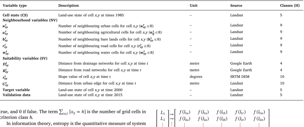
Finally, as there is always a possibility of encountering ‘null’ values using the DoTRules approach where new cells in the test dataset present combinations of criteria states not encountered in the training data. Here, using the same training and test sample, we will sequentially exclude the least informative (i.e. highest entropy and lowest ranked) independent predictor variables orcriteria J′from our analysis and re-execute DoTRules step 3 to 5. This generates a second rule set (i.e. a Table 1

Applied variables including cell state (CS), neighbourhood value (NV), suitability value (SV), target variable and validation data along with a description, units, data source and number of classes (H).

Variable type Description Unit Source Classes (H)

Cell state (CS) Land-use state of cellx,yat times 1985 – Landsat 5

Neighbourhood variables (NV)

uxyt Number of neighbouring urban cells for cellx,y(uxyt≤8) – Landsat 9 axyt Number of neighbouring agricultural cells for cellx,y(aijt≤8) – Landsat 9

bxyt Number of neighbouring bare lands cells for cellx,y(bxyt≤8) – Landsat 9 rxyt Number of neighbouring road cells for cellx,y(rxyt≤8) – Landsat 9 wxyt Number of neighbouring water cells for cellx,y(wxyt≤8) – Landsat 9 Suitability variables (SV)

Dxyt Distance from drainage networks for cellx,yat timet metre Google Earth 4

Rxyt Distance from road networks for cellx,yat timet metre Google Earth 4

sxyt Slope value of cellx,yat timet degrees SRTM DEM 10

Uxyt Distance from urban edge for cellx,yat timet metre Landsat 10

Target variable Land-use state of cellx,yat time 2000 – Landsat 5

sub-rule set) which contains fewer unique rulesd'(in the corresponding

D′)and ‘null’ records as it contains fewer criteria classes. We then re-peat in developing some new sub-rule sets until all ‘null’ values in our primary rule set are covered by some corresponding sub-rules among secondary sub-rule sets. The best sub-rule to replace a null-matching rule in our test rule set is the one with the lowest entropy while those rules with higher entropy values (higher than the specified threshold) are eliminated.

3. Methods

3.1. Study area

The study area was the Ahvaz region of south-west Iran. Ahvaz city is the capital and largest city of Khuzestan province (Fig. 1). The po-pulation of Ahvaz increased from 334,399 to 1,338,126, from 1976 to 2015, with attendant growth in urban areas. The Karun River, 850 km long and Iran's largest, splits the city into western and eastern parts then joins the Arvand Rood River and continues toward the Persian Gulf. The climate is semi-arid, with a mean annual precipitation of 252 mm and an average annual temperature of 26.9 °C. June is the driest and warmest month and January is wettest and coolest.

The major land-use transition trends in the study area included the rapid growth of built-up urban areas (transformed from bare lands and agricultural lands) and agricultural lands (transformed from bare lands) from 1985 up to 2015. A minor transition from agricultural lands to bare lands was also observed. Urban growth was driven by rapid po-pulation growth. Agricultural production has increased to meet in-creasing local demand, supported by the abundance of water and fertile soils. Various agricultural commodities are produced such as wheat, barley, oilseeds, rice, sugar cane, medicinal herbs, as well as orchard crops such as palm, citrus, and olives (Rangzan et al., 2008).

3.2. LUCC simulation process overview

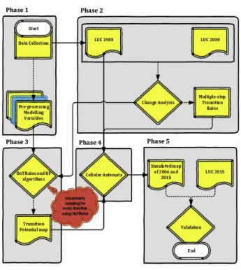
LUCC simulation was implemented in five Phases (Fig. 2). Phase 1 involved data collection, preparation, and pre-processing, including land-use/cover classification, undertaken using geospatial analysis software (ENVI and ArcGIS). Neighbourhood analysis, cost-distance layer preparation, and data discretisation was then done using theraster

package (Hijmans and van Etten, 2014) in R. Phase 2 involved calcu-lating rates of land-use change between 1985 and 2000 and identifying major land-use change transitions for specifying land-use change de-mand (Islam et al., 2018;Kamusoko and Gamba, 2015).

Phase 3 involved the use of DoTRules and random forest (RF) al-gorithms to calculate LUCC transition potential maps using a training sample of randomly selected grid cells. In Phase 4, the land-use map of 1985, transition potential maps, and the estimated rates of land-use change for the primary land-use classes were integrated into a cellular automata model in R. The CA model was calibrated to apply 30 annual iterations (one for each year 1985–2015). Finally, in Phase 5, the pre-dictive accuracy of the simulated land-use maps for 2015 was validated against the classified land-use map for the same year using 100,000 random points for three simulated land-use classes (i.e. urban, agri-culture and bare lands). Finally, we then compared the accuracy of cellular automata land-use change models calibrated using DoTRules and RF algorithms.

3.3. LUCC modelling variables and data sources

image for 2015 was used for validation. Five groups of variables in-cluding cell state (CS), neighbourhood variables (NV), suitability vari-ables (SV), a target variable, and validation data were extracted from the main data sources for LUCC simulation (Table 1).

Note that for the NV, as neighbourhood configuration is known to affect cellular automata simulation (Fuglsang et al., 2013;Lauf et al., 2012; Verstegen et al., 2014;White and Engelen, 1993), the optimal kernel size k= 8 for neighbourhood analysis was selected based on initial cross-validation. All variables were resampled to the 30-m grid cell resolution of the Landsat data, totalling 734,328 cells across the study area. The derivation and use of these variables is described in detail below.

3.3.1. Landsat archive and image classification

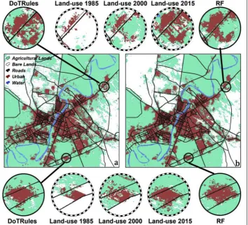
Image pre-processing involved normalization for the region of in-terest. Land-use/cover maps of the study area were then classified using a support vector machine classifier with geospatial analysis software (ENVI and ArcGIS), achieving an overall accuracy of ≥85%. During this process, all grid cells were allocated to one of five land-use/cover classes: urban area, agricultural land, bare land, roads, and water bodies for the 1985, 2000 and 2015 images (Fig. 3).

3.4. Land-use change analysis to compute transition demand

The rate of simulated land-use change, or transition demand, in

cellular automata models needs to be calibrated to observed rates by quantifying the historical amount of change for each land-use type (Hewitt and Díaz-Pacheco, 2017;Kamusoko et al., 2009;Kamusoko and Gamba, 2015;Pastor et al., 1991). We calculated transition demand based on the Landsat-derived land use/cover maps for 1985 and 2000 (Fig. 3). The type and frequency of land-use change between 1985 and 2000 were cross-tabulated. The time interval used for calibration for the 1985–2000 transition matrix was 15 years. Land-use transition probabilities were calculated as average annual rates of change fol-lowing previous studies (Hewitt and Díaz-Pacheco, 2017) in order to take account of annual change demand for each cellular automata iteration.

3.5. Computation of land use/cover transition potential maps

implemented in the randomForest package (Liaw and Wiener, 2002) available in R. CS, NV, and SV were recalculated each year based on the simulated land-use and used to update the land-use transition potential map each year.

3.6. CA-based land-use change simulation

In traditional cellular automata models, the evolution of the future cell state is determined by the following formula (Al-shalabi et al., 2013;Martinez et al., 2012;Wu, 1998):

Sxyt+1=f Sxyt, xyt, xyt

(6) where,Sxyt represents the land-use state for a cell at location (x,y) at

timet. xytis composed of a set of suitability measures for the cell at time t. xytis the state of neighbouring cells at time t, andfis a transition function.

Three datasets, (1) the initial land use/cover map (1985); (2) the transition potential maps (1985–2000); and (3) the transition demand, were used to simulate land use/cover up to 2015 using a cellular au-tomata (Hewitt et al., 2013). Transition demand, calculated via the land-use change analysis, determined the amount of land-use change in each simulated year, while the land-use transition potential determined the location and type of change (Yang et al., 2016). For each simulation year, land-use was allocated by finding the grid cell with the maximum transition potential. If the new land-use was less than that demanded then the change was made. The cell with the next highest transition potential was then found and the change made if the new land-use was less than that demanded. This process was repeated until all land-use demands were met for that year (Yang et al., 2016). This whole process was repeated for 30 annual iterations to simulate land-use from 1985 to 2015 where a new land-use map is produced at the end of each itera-tion.

3.7. Comparing DoTRules with random forests

To quantify DoTRules' performance in calculating land-use transi-tion potential, we implemented the same CA-based LUCC simulatransi-tion scheme but using the RF algorithm (Kamusoko and Gamba, 2015) to calculate transition rules. The RF algorithm provides an appropriate

benchmark for assessing the performance of the DoTRules scheme be-cause of the high performance typically found in predictive modelling (Caruana and Niculescu-Mizil, 2006). RF is also computationally effi-cient and suitable for large training data (Mahapatra, 2014). We com-pared the overall accuracy of both DoTRules and RF-based cellular automata simulation of LUCC for the Ahvaz study area.

4. Results

4.1. Variable importance and transition rules

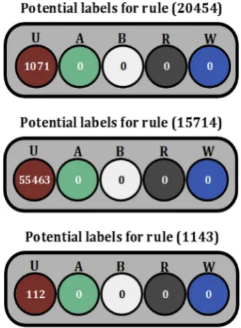
A major product of DoTRules is calculated Shannon entropy values, which are used for prioritising criteria before assembling transition rules. Criteria are ranked and prioritised according to their average entropyej(Equation(3)) with higher priority criteria being those with the lower entropy (Table 2). In our case study, 24,437 transition rules were assembled and applied for the purpose of LUCC simulation. Here, every single rule/sub-rule is defined by a unique string which re-presents criteria values, along with a frequency distribution of potential land-use class labels, rule-exclusive hit ratio, rule-exclusive entropy value, and mode land-use label (Fig. 4).

The transparency of DoTRules opens up information contained in the transition rules for critical observation or examination. For ex-ample, retained information in the following rules of Fig. 4 can be dissected and retrieved once the variable priority is clarified. Here, both rules have the same value for cell state, neighbouring agricultural cells, distance to road, distance to drainage, and neighbouring water and road cells. However, the rules have different values for neighbouring bare land cells, distance from urban, neighbouring urban cells, and slope. The two rules have the same mode label but different un-certainties and hit ratios.

4.2. Simulation performance

Following the simulation procedure based on the transition poten-tial maps as calculated by DoTRules and RF, the results are mapped and then validated by a 100,000 validation test points of 2015 land-use data map (Fig. 5).

This comparison is done only for simulated land-use classes in-cluding urban, agriculture and bare lands. Considering the fact that Fig. 3.Landsat-derived land-use/cover maps of the study area for (a) 1985, (b) 2000 and (c) 2015.

Table 2

Sorted variables of LUCC model fromTable 1along with their priority value (mean entropyej).

Variable CS b_xyt _Uxyt _a

xyt Rxyt uxyt Dtxy wxyt rxyt sxyt

Priority 1st ₂nd ₃rd ₄th ₅th ₆th ₇th ₈th ₉th ₁₀th

land-use map of 2015 was not involved in the preparation of transition potential maps, the overall accuracy of the LUCC simulation using DoTRules (75.4) was very similar to that based on RF (75.8). Although both algorithms demonstrate broad spatial similarities, LUCC simula-tion results of the Ahvaz study area for the target year of 2015 also display localised differences. Land-use simulation of both DoTRules and RF were promising in identifying, retaining, and preserving the spatial

details of the 2015 land-use/cover maps.

4.3. Uncertainty of major land-use transitions

A key advantage of DoTRules is that all major transitions can be identified and dissected, enabling the analysis of major trends of change/persistence along with their corresponding information such as Fig. 4.Samples of low uncertainty (a, left) and high uncertainty (b, right) rules extracted using DoTRules. The string of numbers highlighted in grey is represents concatenated class labels from the 10 variables fromTable 1prioritised by their predictive ability as shown inTable 2.

uncertainty and frequency (Table 3). In terms of land-use change/per-sistence transitions and their uncertainty values, ‘bare lands to bare lands’ persistence had the lowest transition rule uncertainty, while ‘agriculture to urban’ change was the most uncertain land-use transi-tion. Transition rules indicating land-use persistence tended to have lower uncertainty than did rules indicating a change from one land-use to another.

4.4. Rule-level spatial uncertainty

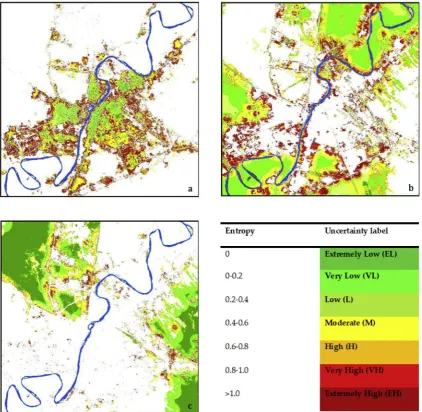
The DoTRules spatial uncertainty product can facilitate the better understanding of uncertainty of transition rules in the mapped land-use predictions. As there will be one uncertainty map for every simulation year, it helps to understand where LUCC simulation results are less or more reliable for each iteration. Considering the results of LUCC si-mulation using DoTRules, the mean uncertainty maps (for 30 iterations) demonstrates a large extent of low (L), very low (VL) and extremely low (EL) uncertainty classes (i.e. class labels) characterised by a low un-certainty estimate may be observed within the inner boundaries, where LUCC is less active. Patches of high (H), very high (VH) and extremely high (EH) uncertainty occurred where LUCC is more active, particularly those areas located at the interface between urban and agricultural lands (Fig. 6).

4.5. Uncertainty and accuracy

In this study, 24,437 unique rules were detected for the primary rule set where their relevant hit ratio is measured using available test data of 2015. Uncertainty was closely related to hit ratio (i.e. percent of cor-rectly assigned land-use labels for a rule) of transition rules where the hit ratio of transitions exponentially decreases with increasing un-certainty (R2_{= 0.89). Thus, low uncertainty transitions are associated} with a higher hit ratio (Fig. 7). Lower uncertainty means there is an obvious land-use class (mode land-use class label) for a rule, while high uncertainty reflects that there are several candidate land-use classes for that rule, which results in less accurate land-use prediction.

5. Discussion

5.1. DoTRules for LUCC simulation

The method used to calculate transition potential maps greatly af-fects the performance of automata-based LUCC models (Charif et al., 2012;Mas et al., 2014;van Vliet et al., 2016). Transparency and un-certainty of the transition rules are important for providing a better understanding of the model structure and of the nature of land-use transitions. Here, we introduced and applied a competent and trans-parent algorithm for the calculation of LUCC transition potential maps for use in cellular automata modelling of land-use change. As a pre-dictive algorithm, DoTRules represents a new way to extract transition rules and map transition potential for use in LUCC simulation models

while also enabling the mapping of uncertainty values at both pixel and rule levels. This makes uncertainty explicit and opens up the informa-tion contained in the transiinforma-tion rules to better model scrutiny and to better-informed land-use planning and policymaking. The potential of DoTRules is demonstrated here for the Ahvaz study area, and more applications and experiments are now required in different geographic contexts to fully explore the general applicability of DoTRules as a land-use transition rule detection algorithm. Below we discuss expand on the advantages and limitations of using DoTRules for cellular automata-based LUCC simulation.

5.1.1. Transparency of transition rules

Depending on the method used to extract transition rules, some rule sets may be omitted which impairs the quality of the transition po-tential map and subsequent LUCC simulation. For instance, in applying black-box algorithms such as RF to calculate LUCC transition potential, it is difficult, if not impossible, to interpret the derived relationships between future land-use and predictor variables such as cell state, neighbourhood, and suitability variables. As a result, we cannot gain a clear understanding of the problem at hand due to the lack of an ex-planatory capability to provide insight into the characteristics of the target dataset (Qiu and Jensen, 2004). The aim of developing and ap-plying DoTRules for LUCC simulation was to improve the quality of urban planning by identifying reliable and accessible land-use transi-tion rules. DoTRules provides an opportunity to uncover model struc-ture by adding more clarity to implemented transition rules and re-vealing information such as rules component priority order and values, frequency distribution of potential matching land-use labels for every rule, and rule-exclusive hit ratio and uncertainty (Fig. 4). It can also identify simplified sub-rule sets compromising only the more in-formative variables. For instance, considering major types of land-use change/persistence, DoTRules identifies the rules governing the most common change/persistence patterns within the study area. Land-use planners and policy makers can explore alternative possibilities for land-use if past transparent and well-understood land-use transition rules continue into the future. A transparent set of land-use transition rules can also help uncover model structure hidden by other black-box algorithms and aid model verification and error identification (Bauer and Steinnocher, 2001; Tseng et al., 2008). Although most LUCC modellers are aware of the shortcomings and the limited accuracy of their input data, very little is known about the propagation of such errors in LUCC models (Dong et al., 2015).

5.1.2. Uncertainty of transition rules

We have demonstrated DoTRules' ability to quantify the frequency and uncertainty of land-use transition rules (Table 3; Fig. 4). It is beneficial to gain reliable information corresponding to the function-ality of those rules including their uncertainty and their corresponding hit ratio (Fig. 4). Regardless of the fact that a rule is indicating the change or persistence of land-use in a grid cell, the rule-level un-certainty values provide a strong indication of prediction hit ratio and Table 3

can be applied as a filter to remove low accuracy portions of a LUCC map derived from unreliable transitions.

The uncertainty of rules belonging to primary land-use transitions

(Table 3) is also useful for the prior exploration of potential accuracy values (i.e. accuracy estimate) and can reduce or eliminate the need for post-hoc validation. This can be done for the primary rule set or a sub-rule set extracted from training data focusing on some specific land-use variables forming land-use transition potential maps. DoTRules' rule-level uncertainty product contains detailed information about the multiple specific land-use transitions in a study area, which provide landscape and urban planners with the opportunity to better under-stand the nature of future land-use transitions and the level of con-fidence in their prediction. For instance, considering the results of un-certainty assessment for LUCC simulation (Fig. 6andTable 3), the land-use transition between urban and agriculture/bare lands is more un-certain than simulated land-use transitions between agricultural lands and bare lands. By specifying uncertainty thresholds, land-use transi-tions in which we are most confident or least confident can be identi-fied, and these can be made explicit in mapped planning outputs to guide decision-making. Thereby, uncertainty thresholds may be applied to any type of transitions for reducing the rule population to include only the most trusted (i.e. those below a specific uncertainty value). The high degree of correspondence between uncertainty and hit ratio means that planners can use DoTRules' uncertainty products as an indicator of land-use simulation accuracy. For example, if the uncertainty threshold Fig. 6.Uncertainty map of DoTRules for three major land-use classes including (a) urban, (b) agriculture, (c) bare lands, during 30 years of simulation (up to 2015) in the study area.

of 0.2 is applied, then planners can be confident that the hit ratio of all the remaining rules should be high (i.e. above 90%) (Fig. 7).

5.1.3. Mapping uncertainty

In addressing the limitations of widely used accuracy measures and indices, using the DoTRules algorithm, we can also map and apply lo-calised uncertainty values within different classification stages as an estimate of accuracy. Thus, a strength of DoTRules in LUCC modelling is its demonstrated ability to quantify the uncertainty of simulated land-use patterns at pixel level, regardless of test data availability. Uncertainty maps can be produced as an estimate of prediction accu-racy even for future land-use change scenarios which lack ground truth data. This enables the most recent data to be used in model-building rather than model validation, which should produce more reliable land-use simulation further into the future, yet still providing an estimate of uncertainty. Spatially-explicit uncertainty also assists landscape and urban planners to foresee the degree of susceptibility to prediction error for specific localities. Rule-level uncertainty maps are created for every LUCC iteration (30 iterations in the present study), as every pixel cor-responds to one transition rule for every iteration. The mean un-certainty of these transition rules allocated to a single grid cell may be calculated, mapped and analysed for one or many iterations. Uncertainty values vary over time for LUCC simulation for each pixel and this can be graphed over time. This helps landscape and urban planners to keep track of LUCC modelling uncertainty and/or hit ratio at pixel level at different time steps of a LUCC model. Other indicators of uncertainty may also be produced including the maximum, minimum, or median; each of which may be useful, depending on the planning application.

5.2. Broader application to environmental modelling

DoTRules quantifies the level of correspondence between each predictor variable and response variable (Table 1) through the calcu-lation of entropy values (Equation(3)). In addition, it also extracts the transparent rules, each with a quantified frequency and entropy, which provides insight into the observed dynamics (Table 3). In this paper, we have applied DoTRules for calculating transition potential in cellular automata models of land-use/cover change. Nonetheless, the con-ceptual framework of DoTRules can be applied to other applications of automata models such as plant population dynamics, forest/bush fire spreading, slope failure, debris flow, and urban sprawl where transition potential mapping is required and where it is necessary to understand the direction and magnitude of state transitions with greater transpar-ency. For instance, in terms of bushfire simulation using cellular au-tomata, a same set of transition rules should be determined to form a transition potential map (Quartieri et al., 2010) while different set of predictor variables such as bush density, flammability, land height and wind (Li and Magill, 2001). Simultaneously, the application of rule-base methods such as DoTRules-for a better understanding of dynamic en-vironmental phenomena is not limited to automata models (Amini et al., 2010; Luo et al., 2017; Moore et al., 2014) and it involves a broader range of environmental models. The authors are currently trialling DoTRules in other critical applications such as image classifi-cation and landslide susceptibility zonation.

5.3. Limitations of DoTRules

The major limitation of DoTRules corresponds with the calculated entropy value for low-frequency rules where, in calculating Shannon entropy values, some rules may be attributed a low-uncertainty value by chance, due to a very low-frequency value. For instance, if the en-tropy value of two different rules is equal, they would be attributed the same uncertainty class. Nonetheless, they may be different in terms of frequency values (Fig. 8). In this regard, among the rules with the same entropy values, those with higher frequency would be more reliable as

they occurred more often. A subjective thresholding approach may be beneficial to deal with this problem. Thus, those low-frequency rules should be ignored if they belong to a frequency value lower than a threshold defined by the user.

6. Conclusion

Cellular automata have long been used to capture the complex dy-namics of LUCC processes. We have presented a new and innovative algorithm called DoTRules—Dictionary of Trusted Rules—for calcula-tion of transicalcula-tion rules and transicalcula-tion potential maps for use in CA-based simulation models. We have then presented an application of the pro-posed approach in the context of LUCC simulation where cellular au-tomata models are increasingly popular. DoTRules enables land-use allocation to be implemented with a new level of transparency and transition rule characteristics are accessible and can be monitored. DoTRules also enables the spatial exploration of LUCC prediction un-certainty. These estimates can assist urban planners in avoiding risky land-use predictions where rules are not reliable. Assessing rule in-formation also enables the detection of trends and understanding pro-cesses of land-use change in a study area. The performance of automata simulation based on DoTRules transition potential calculation was very similar to simulation based on the state-of-the-art random forest method. Hence, we conclude that DoTRules is a promising approach for extraction of transition rules and providing transition potential maps for CA-based simulation due to its predictive ability, transparency, and ability to produce multiple uncertainty products. These capabilities can enhance the utility of automata-based simulation as a tool for end-users and improve the quality of the resultant decision-making process. More experiments in different environmental applications with a different set of variables are now required to verify the broader utility of DoTRules as a CA calibration tool. The application of DoTRules as a transparent rule-based approach to other environmental modelling applications should also be explored.

6.1. Software availability

preparation and processing, land-use simulation and map creation. DoTRules script is implemented in R v. 3.5.0.

•

•

•

Note: No specific software component has been developed for this study.

Acknowledgements

This research was supported by CSIRO Australian Sustainable Agriculture Scholarship (ASAS) as a top-up scholarship to Majid Shadman, a PhD scholar in the Discipline of Geography and Spatial Sciences, School of Technology, Environments and Design at the University of Tasmania (RT109121). BAB was supported by Deakin University. We thank three anonymous reviewers for their suggestions for improving the manuscript.

References

Adinarayana, J., Gopal Rao, K., Rama Krishna, N., Venkatachalam, P., Suri, J.K., 1999. A rule-based soil erosion model for a hilly catchment. Catena 37 (3), 309–318.

Al-shalabi, M., Billa, L., Pradhan, B., Mansor, S., Al-Sharif, A.A.A., 2013. Modelling urban growth evolution and land-use changes using GIS based cellular automata and SLEUTH models: the case of Sana'a metropolitan city, Yemen. Environmental Earth Sciences 70 (1), 425–437.

Al‐kheder, S., Wang, J., Shan, J., 2008. Fuzzy inference guided cellular automata ur-ban‐growth modelling using multi‐temporal satellite images. Int. J. Geogr. Inf. Sci. 22 (11–12), 1271–1293.

Amini, M., Abbaspour, K.C., Johnson, C.A., 2010. A comparison of different rule-based statistical models for modeling geogenic groundwater contamination. Environ. Model. Software 25 (12), 1650–1657.

Arsanjani, J.J., Kainz, W., Mousivand, A.J., 2011. Tracking dynamic land-use change using spatially explicit Markov chain based on cellular automata: the case of Tehran. International Journal of Image and Data Fusion 2 (4), 329–345.

Ballestores Jr., F., Qiu, Z., 2012. An integrated parcel-based land use change model using cellular automata and decision tree. Proceedings of the International Academy of Ecology and Environmental Sciences 2 (2), 53.

Basse, R.M., Charif, O., Bódis, K., 2016. Spatial and temporal dimensions of land use change in cross border region of Luxembourg. Development of a hybrid approach integrating GIS, cellular automata and decision learning tree models. Appl. Geogr. 67, 94–108.

Basse, R.M., Omrani, H., Charif, O., Gerber, P., Bódis, K., 2014. Land use changes mod-elling using advanced methods: cellular automata and artificial neural networks. The spatial and explicit representation of land cover dynamics at the cross-border region scale. Appl. Geogr. 53, 160–171.

Bauer, T., Steinnocher, K., 2001. Per-parcel land use classification in urban areas applying a rule-based technique. GeoBIT/GIS 6, 24–27.

Berberoğlu, S., Akın, A., Clarke, K.C., 2016. Cellular automata modeling approaches to forecast urban growth for adana, Turkey: a comparative approach. Landsc. Urban Plann. 153, 11–27.

Breiman, L., 1996. Bagging predictors. Mach. Learn. 24 (2), 123–140.

Breiman, L., 2001. Random forests. Mach. Learn. 45 (1), 5–32.

Bryan, B.A., Barry, S., Marvanek, S., 2009. Agricultural commodity mapping for land use change assessment and environmental management: an application in the Murray–Darling Basin, Australia. J. Land Use Sci. 4 (3), 131–155.

Caruana, R., Niculescu-Mizil, A., 2006. An empirical comparison of supervised learning algorithms. In: Proceedings of the 23rd International Conference on Machine Learning. ACM, pp. 161–168.

Castilla, A., Blas, N.G., 2008. Self–organizing map and Cellular automata combined technique for advanced mesh generation in urban and architectural design. International Journal” Information Technologies and knowledge 2.

Charif, O., Basse, R.-M., Omrani, H., Trigano, P., 2012. Cellular automata model based on machine learning methods for simulating land use change, Simulation Conference (WSC). In: Proceedings of the 2012 Winter. IEEE, pp. 1–12.

Clarke, K.C., Hoppen, S., Gaydos, L., 1997. A self-modifying cellular automaton model of historical urbanization in the San Francisco Bay area. Environ. Plann. Plann. Des. 24 (2), 247–261.

Congalton, R.G., 1991. A review of assessing the accuracy of classifications of remotely sensed data. Remote Sens. Environ. 37 (1), 35–46.

D'Ambrosio, D., Gregorio, S.D., Iovine, G., 2003. Simulating debris flows through a hexagonal cellular automata model: sciddica s 3–hex. Nat. Hazards Earth Syst. Sci. 3 (6), 545–559.

D'Ambrosio, D., Spataro, W., Iovine, G., 2006. Parallel genetic algorithms for optimising cellular automata models of natural complex phenomena: an application to debris flows. Comput. Geosci. 32 (7), 861–875.

Dong, M., Bryan, B.A., Connor, J.D., Nolan, M., Gao, L., 2015. Land use mapping error

introduces strongly-localised, scale-dependent uncertainty into land use and eco-system services modelling. Ecoeco-system services 15, 63–74.

Fuglsang, M., Münier, B., Hansen, H.S., 2013. Modelling land-use effects of future ur-banization using cellular automata: an Eastern Danish case. Environ. Model. Software 50, 1–11.

Gibert, K., Rodríguez-Silva, G., Rodríguez-Roda, I., 2010. Knowledge discovery with clustering based on rules by states: a water treatment application. Environ. Model. Software 25 (6), 712–723.

Han, H., Yang, C., Song, J., 2015. Scenario simulation and the prediction of land use and land cover change in Beijing, China. Sustainability 7 (4), 4260.

Hewitt, R., Díaz-Pacheco, J., 2017. Stable models for metastable systems? Lessons from sensitivity analysis of a Cellular Automata urban land use model. Comput. Environ. Urban Syst. 62, 113–124.

Hewitt, R., Díaz Pacheco, J., Moya Gómez, B., 2013. A Cellular Automata Land Use Model for the R Software Environment.

Hewitt, R., van Delden, H., Escobar, F., 2014. Participatory land use modelling, pathways to an integrated approach. Environ. Model. Software 52, 149–165.

Hijmans, R.J., van Etten, J., 2014. raster: geographic data analysis and modeling. R package version 2 (8).

Islam, K., Rahman, M.F., Jashimuddin, M., 2018. Modeling land use change using cellular automata and artificial neural network: the case of chunati wildlife sanctuary, Bangladesh. Ecol. Indicat. 88, 439–453.

Kamusoko, C., Aniya, M., Adi, B., Manjoro, M., 2009. Rural sustainability under threat in Zimbabwe – simulation of future land use/cover changes in the Bindura district based on the Markov-cellular automata model. Appl. Geogr. 29 (3), 435–447.

Kamusoko, C., Gamba, J., 2015. Simulating urban growth using a Random Forest-Cellular Automata (RF-CA) model. ISPRS Int. J. Geo-Inf. 4 (2), 447–470.

Khatami, R., Mountrakis, G., Stehman, S.V., 2017. Mapping per-pixel predicted accuracy of classified remote sensing images. Remote Sens. Environ. 191, 156–167.

Koomen, E., Borsboom-van Beurden, J., 2012. Land-use Modelling in Planning Practice. Springer.

Ku, C.-A., 2016. Incorporating spatial regression model into cellular automata for simu-lating land use change. Appl. Geogr. 69, 1–9.

Lai, C., Shao, Q., Chen, X., Wang, Z., Zhou, X., Yang, B., Zhang, L., 2016. Flood risk zoning using a rule mining based on ant colony algorithm. J. Hydrol. 542, 268–280.

Lauf, S., Haase, D., Hostert, P., Lakes, T., Kleinschmit, B., 2012. Uncovering land-use dynamics driven by human decision-making–A combined model approach using cellular automata and system dynamics. Environ. Model. Software 27, 71–82.

Li, X., Lao, C., Liu, Y., Liu, X., Chen, Y., Li, S., Ai, B., He, Z., 2013. Early warning of illegal development for protected areas by integrating cellular automata with neural net-works. J. Environ. Manag. 130, 106–116.

Li, X., Liu, X., Gong, P., 2015. Integrating ensemble-urban cellular automata model with an uncertainty map to improve the performance of a single model. Int. J. Geogr. Inf. Sci. 29 (5), 762–785.

Li, X., Magill, W., 2001. Modeling fire spread under environmental influence using a cellular automaton approach. Complex. Int. 8 (1), 1–14.

Li, X., Yeh, A.G.-O., 2002. Neural-network-based cellular automata for simulating mul-tiple land use changes using GIS. Int. J. Geogr. Inf. Sci. 16 (4), 323–343.

Liaw, A., Wiener, M., 2002. Classification and regression by randomForest. R. News 2 (3), 18–22.

Liu, X., Jiang, B., 2011. A novel approach to the identification of urban sprawl patches based on the scaling of geographic space. Int. J. Geomatics Geosci. 2 (2), 415.

Liu, Y., Feng, Y., Pontius, R.G., 2014. Spatially-explicit simulation of urban growth through self-adaptive genetic algorithm and cellular automata modelling. Land 3 (3), 719–738.

Liucci, L., Melelli, L., Suteanu, C., Ponziani, F., 2017. The role of topography in the scaling distribution of landslide areas: a cellular automata modeling approach.

Geomorphology 290, 236–249.

Long, Y., Jin, X., Yang, X., Zhou, Y., 2014. Reconstruction of historical arable land use patterns using constrained cellular automata: a case study of Jiangsu, China. Appl. Geogr. 52, 67–77.

Luo, Y., He, J., He, Y., 2017. A rule-based city modeling method for supporting district protective planning. Sustainable Cities and Society 28, 277–286.

Mahapatra, D., 2014. Analyzing training information from random forests for improved image segmentation. IEEE Trans. Image Process. 23 (4), 1504–1512.

Martinez, G.J., Adamatzky, A., Alonso-Sanz, R., 2012. Complex dynamics of elementary cellular automata emerging from chaotic rules. International Journal of Bifurcation and Chaos 22 (02), 1250023.

Mas, J.-F., Kolb, M., Paegelow, M., Camacho Olmedo, M.T., Houet, T., 2014. Inductive pattern-based land use/cover change models: a comparison of four software packages. Environ. Model. Software 51, 94–111.

Moore, A.D., Holzworth, D.P., Herrmann, N.I., Brown, H.E., de Voil, P.G., Snow, V.O., Zurcher, E.J., Huth, N.I., 2014. Modelling the manager: representing rule-based management in farming systems simulation models. Environ. Model. Software 62, 399–410.

Mustafa, A., Cools, M., Saadi, I., Teller, J., 2017. Coupling agent-based, cellular automata and logistic regression into a hybrid urban expansion model (HUEM). Land Use Pol. 69, 529–540.

Mustafa, A., Heppenstall, A., Omrani, H., Saadi, I., Cools, M., Teller, J., 2018a. Modelling built-up expansion and densification with multinomial logistic regression, cellular automata and genetic algorithm. Comput. Environ. Urban Syst. 67, 147–156.

Mustafa, A., Rienow, A., Saadi, I., Cools, M., Teller, J., 2018b. Comparing support vector machines with logistic regression for calibrating cellular automata land use change models. European Journal of Remote Sensing 51 (1), 391–401.

Sciences, pp. 5–28.

Pontius Jr., R.G., Millones, M., 2011. Death to Kappa: birth of quantity disagreement and allocation disagreement for accuracy assessment. Int. J. Rem. Sens. 32 (15), 4407–4429.

Pozoukidou, G., 2005. Increased Usability of Urban and Land Use Models. The Role of Knowledge Based Systems in Facilitating Land Use Forecasting to Planning Agencies.

Qiu, F., Jensen, J., 2004. Opening the black box of neural networks for remote sensing image classification. Int. J. Rem. Sens. 25 (9), 1749–1768.

Quartieri, J., Mastorakis, N.E., Iannone, G., Guarnaccia, C., 2010. A cellular automata model for fire spreading prediction. Latest Trends on Urban Planning and Transportation 173–178.

R Core Team, 2017. R: a Language and Environment for Statistical Computing.

Rangzan, K., Sulaimani, B., Sarsangi, A., Abshirini, A., 2008. Change detection, miner-alogy, desertification mapping in East and Northeast of Ahvaz City, SW Iran using combination of remote sensing methods, GIS and ESAS model. Global J. Environ. Res. 2 (1), 42–52.

Rienow, A., Goetzke, R., 2015. Supporting SLEUTH – enhancing a cellular automaton with support vector machines for urban growth modeling. Comput. Environ. Urban Syst. 49, 66–81.

Royston, S.J., Horsburgh, K.J., Lawry, J., 2012. Application of rule based methods to predicting storm surge. Continent. Shelf Res. 37, 79–91.

Russell, S.J., Norvig, P., Canny, J.F., Malik, J.M., Edwards, D.D., 2003. Artificial Intelligence: a Modern Approach, 2. Prentice hall Upper Saddle River.

Shadman Roodposhti, M., Aryal, J., Shahabi, H., Safarrad, T., 2016. Fuzzy shannon en-tropy: a hybrid GIS-based landslide susceptibility mapping method. Entropy 18 (10), 343.

Shannon, C.E., 2001. A mathematical theory of communication. ACM SIGMOB - Mob. Comput. Commun. Rev. 5 (1), 3–55.

Stein, A., Aryal, J., Gort, G., 2005. Use of the Bradley-Terry model to quantify association in remotely sensed images. IEEE Trans. Geosci. Rem. Sens. 43 (4), 852–856.

Tayyebi, A.H., Tayyebi, A., Khanna, N., 2014. Assessing uncertainty dimensions in land-use change models: using swap and multiplicative error models for injecting attribute and positional errors in spatial data. Int. J. Rem. Sens. 35 (1), 149–170.

Tseng, M.-H., Chen, S.-J., Hwang, G.-H., Shen, M.-Y., 2008. A genetic algorithm rule-based approach for land-cover classification. ISPRS J. Photogrammetry Remote Sens. 63 (2), 202–212.

Tsutsumida, N., Comber, A.J., 2015. Measures of spatio-temporal accuracy for time series land cover data. Int. J. Appl. Earth Obs. Geoinf. 41, 46–55.

Uzuner, Ö., Zhang, X., Sibanda, T., 2009. Machine learning and rule-based approaches to assertion classification. J. Am. Med. Inf. Assoc. 16 (1), 109–115.

van Vliet, J., Bregt, A.K., Brown, D.G., van Delden, H., Heckbert, S., Verburg, P.H., 2016. A review of current calibration and validation practices in land-change modeling. Environ. Model. Software 82, 174–182.

Van Vliet, J., White, R., Dragicevic, S., 2009. Modeling urban growth using a variable grid cellular automaton. Comput. Environ. Urban Syst. 33 (1), 35–43.

Vaz, E., Arsanjani, J.J., Phillips, L., Johnson, M., Deener, K., Bonanni, C., Xia, X., Wu, Q., Mou, X., Lai, Y., 2015. Predicting urban growth of the greater toronto area-coupling a markov cellular automata with document meta-analysis. Journal Of Environmental Informatics 25 (2), 71–80.

Verstegen, J.A., Karssenberg, D., van der Hilst, F., Faaij, A.P.C., 2014. Identifying a land use change cellular automaton by Bayesian data assimilation. Environ. Model. Software 53, 121–136.

Waddell, P., 2002. UrbanSim: modeling urban development for land use, transportation, and environmental planning. J. Am. Plann. Assoc. 68 (3), 297–314.

White, R., Engelen, G., 1993. Cellular automata and fractal urban form: a cellular mod-elling approach to the evolution of urban land-use patterns. Environ. Plann. 25 (8), 1175–1199.

White, R., Engelen, G., 1997. Cellular automata as the basis of integrated dynamic re-gional modelling. Environ. Plann. Plann. Des. 24 (2), 235–246.

Wu, F., 1998. Simulating urban encroachment on rural land with fuzzy-logic-controlled cellular automata in a geographical information system. J. Environ. Manag. 53 (4), 293–308.

Xu, J., Gu, B., Guo, Y., Chang, J., Ge, Y., Min, Y., Jin, X., 2010. A cellular automata model for population dynamics simulation of two plant species with different life strategies, Intelligent Systems and Knowledge Engineering (ISKE). In: 2010 International Conference on. IEEE, pp. 517–523.

Yang, J., Su, J., Chen, F., Xie, P., Ge, Q., 2016. A local land use competition cellular automata model and its application. ISPRS Int. J. Geo-Inf. 5 (7), 106.

Yang, Q., Li, X., Shi, X., 2008. Cellular automata for simulating land use changes based on support vector machines. Comput. Geosci. 34 (6), 592–602.

Zhang, X., Tong, X., Liu, M., 2008. Genetic algorithm optimized neutral network classi-fication and overlapping pixel change detection based on remote sensing for urban sprawl: a case study in Jiading district of Shanghai, China. In: Proceedings of the ISPRS XXIst Congress, July, pp. 3–11.