Gradient Tree Boosting for Training Conditional Random Fields

Gradient Tree Boosting for Training Conditional Random Fields

Thomas G. Dietterich [email protected]

Guohua Hao [email protected]

School of Electrical Engineering and Computer Science Oregon State University

Corvallis, OR 97331, USA

Adam Ashenfelter [email protected]

Cleverset, Inc.

Corvallis, OR 97330, USA

Editor: Michael Collins

Abstract

Conditional random fields (CRFs) provide a flexible and powerful model for sequence labeling problems. However, existing learning algorithms are slow, particularly in problems with large numbers of potential input features and feature combinations. This paper describes a new algo-rithm for training CRFs via gradient tree boosting. In tree boosting, the CRF potential functions are represented as weighted sums of regression trees, which provide compact representations of feature interactions. So the algorithm does not explicitly consider the potentially large parameter space. As a result, gradient tree boosting scales linearly in the order of the Markov model and in the order of the feature interactions, rather than exponentially as in previous algorithms based on iterative scaling and gradient descent. Gradient tree boosting also makes it possible to use instance weighting (as in C4.5) and surrogate splitting (as in CART) to handle missing values. Experimental studies of the effectiveness of these two methods (as well as standard imputation and indicator fea-ture methods) show that instance weighting is the best method in most cases when feafea-ture values are missing at random.

Keywords: sequential supervised learning, conditional random fields, functional gradient,

gradi-ent tree boosting, missing values

1. Introduction

Many applications of machine learning involve assigning labels collectively to sequences of objects. For example, in natural language processing, the task of part-of-speech (POS) tagging is to label each word in a sentence with a part of speech tag (“noun”, “verb” etc.) (Ratnaparkhi, 1996). In computational biology, the task of protein secondary structure prediction is to assign a secondary structure class to each amino acid residue in the protein sequence (Qian and Sejnowski, 1988).

We call this class of problems sequential supervised learning (SSL), and it can be formulated as follows:

Find: A classifier H that, given a new sequence X of feature vectors, predicts the corresponding sequence of class labels Y =H(X)accurately.

Perhaps the most famous SSL problem is the NETtalk task of pronouncing English words by assigning a phoneme and stress to each letter of the word (Sejnowski and Rosenberg, 1987). Other applications of SSL arise in information extraction (McCallum et al., 2000) and handwritten word recognition (Taskar et al., 2004).

Early attempts to apply machine learning to SSL problems were based on sliding windows. To predict label yt, a sliding window method uses features drawn from some “window” of the X

sequence. For example, a 5-element window wt(X)would use the features xt−2,xt−1,xt,xt+1,xt+2. Sliding windows convert the SSL problem into a standard supervised learning problem to which any ordinary machine learning algorithm can be applied. However, in most SSL problems, there are correlations among successive class labels yt. For example, in part-of-speech tagging, adjectives

tend to be followed by nouns. In protein sequences, alpha helixes and beta structures always involve multiple adjacent residues. These correlations can be exploited to increase classification accuracy.

The best-known method for capturing the yt−1 ↔yt correlation is the hidden Markov model

(HMM) (Rabiner, 1989), which is a generative model of P(X,Y), the joint distribution of the ob-servation sequence and label sequence. In this model, the joint distribution is factored as P(X,Y) = ∏tP(yt|yt−1)P(xt|yt), and the observation distribution is further factored as P(xt|yt) =∏jP(xt,j|yt).

This assumption of independence of each input feature xt,j conditioned on yt makes HMMs unable

to model arbitrary, non-independent input features, and this limits the accuracy and “engineerabil-ity” of HMMs.

Recent research has instead focused on discriminative models, in which arbitrary and non-independent observation features can be easily incorporated. Much machine learning research has shown that discriminative models tend to be more accurate and more robust to incorrect modeling assumptions (Ng and Jordan, 2002). McCallum and his collaborators introduced maximum entropy Markov models (MEMMs) (McCallum et al., 2000) and conditional random fields (CRFs) (Lafferty et al., 2001). MEMMs are directed graphical models of the form P(Y|X) =∏_tP(yt|yt−1,wt(X)),

where wt(X)is a sliding window over the X sequence. They are easy to train, but they suffer from

the label bias problem that results from the local normalization at each time step t. Conditional random fields are undirected models of the form P(Y|X) =1/Z(X)exp∑_tΨ(yt,yt−1,wt(X)), where

Z(X)is a global normalizing term andΨ(yt,yt−1,wt(X))is a potential function that scores the

com-patibility of yt, yt−1, and wt(X). The global normalization avoids the label bias problem but makes

training much more computationally expensive. CRFs have been applied to many problems with excellent results including POS tagging (Lafferty et al., 2001) and noun-phrase chunking (Sha and Pereira, 2003).

Kernel-based methods have also been extended to the SSL case. The hidden Markov SVM (Al-tun et al., 2003; Tsochantaridis et al., 2004) and max-margin Markov networks (Taskar et al., 2004) learn a discriminant function F(X,Y0) that assigns a real valued score to each possible label se-quence Y0to maximize the margin between the correct label sequence Y and all competing incorrect label sequences.

Training CRFs is difficult for several reasons. First, as with all collective classification problems, training requires performing inference. In particular, all algorithms must compute the conditional log likelihood log P(Yi|Xi)for each training example(Xi,Yi)in each iteration. This is expensive, and

features for describing the arguments ofψ(i.e., yt, yt−1, and wt(X)) is immense. Even in the simple

case whereψis represented as a simple linear function W·F(yt,yt−1,wt(X)), there can be millions

of weights to learn in W . In POS tagging and semantic role labeling, for example, it is common to have one feature (and hence, one weight) for every combination of a word and a pair of class labels. Furthermore, in most applications, performance is improved if the algorithm can consider combinations of these basic features (e.g., word n-grams, feature conjunctions and disjunctions, etc.). If feature interactions are permitted, the number of parameters to be learned explodes. Finally, in some problems, feature values can be missing, and this is difficult for discriminative training algorithms to handle.

There has been steady progress in algorithms for training CRFs. The initial paper (Lafferty et al., 2001) introduced an iterative scaling algorithm, which was reported to be exceedingly slow. Several groups have implemented gradient ascent methods (such as Sha and Pereira, 2003), but naive implementations are also very slow. McCallum’s Mallet system (McCallum, 2002) employs the BFGS algorithm, which is an approximate second order method, to speed up the training of CRFs and improve the prediction accuracy. More recently, Vishwanathan et al. (2006) proposed to use stochastic gradient method to train CRFs, and accelerate this process via the Stochastic Meta-Descent (SMD), which is a gain adaptation method. The resulting algorithm is much faster than the BFGS algorithm and scales well on large data sets.

In this paper, we introduce a different approach for training the potential functions based on Friedman’s gradient tree boosting algorithm (Friedman, 2001). In this method, the potential func-tions are represented by sums of regression trees, which are grown stage-wise in the manner of Adaboost (Freund and Schapire, 1996). Because each iteration adds an entire regression tree to the potential function, each iteration can take a big step in parameter space, and hence, reduce the number of iterations needed. Tree boosting also addresses the problem of dealing with feature in-teractions. Each regression tree can be viewed as defining several new feature combinations—one corresponding to each path in the tree from the root to a leaf. The resulting potential functions still have the form of a linear combination of features, but the features can be quite complex. Another advantage of tree boosting is that it is able to handle missing values in the inputs using clever meth-ods specific to regression trees, such as the instance weighting method of C4.5 (Quinlan, 1993) and the surrogate splitting method of CART (Breiman et al., 1984). Finally, the algorithm is fast and straightforward to implement. In addition, there may be some tendency to avoid overfitting because of the “ensemble effect” of combining multiple regression trees.

This paper describes the gradient tree boosting algorithm including methods for incorporating weight penalties into the procedure. It then compares training time and generalization performance against McCallum’s Mallet system. The results show that our implementation of tree boosting is competitive with Mallet in both speed and accuracy and that additional improvements in our implementation of the forward-backward algorithm would likely produce a system that is faster than both systems. We also perform experiments to evaluate the effectiveness of four methods for handling missing values (instance weighting, surrogate splits, indicator features, and imputation). The results show that instance weighting works best, but that imputation also works surprisingly well.

2. Conditional Random Fields

Let(X,Y) be a sequential labeled training example, where X= (x1, . . . ,xT)is the observation

se-quence and Y = (y1, . . . ,yT)is the sequence of labels, where yt ∈ {1, . . . ,K)for all t. A conditional

random field is a linear chain Markov random field (Geman and Geman, 1984) over the label se-quence Y globally conditioned on the observation sese-quence X . The probability distribution can be written as

P(Y|X) = 1

Z(X)exp

∑

t

Ψt(yt,X) +Ψt−1,t(yt−1,yt,X)

,

where Ψt(yt,X) and Ψt−1,t(yt−1,yt,X) are potential functions that capture (respectively) the

de-gree to which yt is compatible with X and the degree to which yt is compatible with a

tran-sition from yt−1 and with X . These potential functions can be arbitrary real-valued functions. The exponential function ensures that P(Y|X) is positive, and the normalizing constant Z(X) = ∑Y0exp[∑tΨt(y0t,X) +Ψt−1,t(y_t0₋₁,yt0,X)]ensures that P(Y|X) sums to 1. If given sufficiently rich

potential functions, this model can represent any first-order Markov distribution P(Y|X)subject to the assumption that P(Y|X)>0 for all X and Y (Besag, 1974; Hammersley and Clifford, 1971). Normally, it is assumed that the potential functions do not depend on t, and we will adopt this assumption in this paper.

To apply a CRF to an SSL problem, we must choose a representation for the potential functions. Lafferty et al. (2001) studied potential functions that are weighted combinations of binary features:

Ψt(yt,X) =

∑

βaga(yt,X) ,

Ψt−1,t(yt−1,yt,X) =

∑

λbfb(yt−1,yt,X) ,

where theβa’s andλb’s are trainable weights, and the features ga and fb are boolean functions. In

part-of-speech tagging, for example, g234(yt,X)might be 1 when xt is the word “bank” and ytis the

class “noun” (and 0 otherwise). As with sliding window methods, it is natural to define features that depend only on a sliding window wt(X)of X values. This linear parameterization can be seen as an

extension of logistic regression to the sequential case.

CRFs can be trained by maximizing the log likelihood of the training data, possibly with a regularization penalty to prevent overfitting. Let Θ={β1, . . . ,λ1, . . .} denote all of the tunable parameters in the model. Then we seek to maximize the objective function

J(Θ) = log

∏

i

P(Yi|Xi)

=

∑

i

log 1 Z(Xi)

exp

∑

t

Ψt(yi,t,Xi) +Ψt−1,t(yi,t−1,yi,t,Xi)

=

∑

i

∑

Ψt(yi,t,Xi) +Ψt−1,t(yi,t−1,yi,t,Xi)−log Z(Xi)

=

∑

i

∑

∑

βaga(yi,t,Xi) +

∑

λbfb(yi,t−1,yi,t,Xi)−log Z(Xi) .

of features, and hence, in the dimensionality of the optimization problem. For example, in protein secondary structure prediction, Qian and Sejnowski (1988) found that a 13-residue sliding window gave best results for neural network methods. There are 32×13×20=2340 basic fbfeatures that

can be defined over this window. If we consider fourth-order conjunctions of such features, we obtain more than 1012features. This is obviously infeasible.

McCallum’s Mallet system (McCallum, 2002) implements standard CRFs and CRFs with fea-ture induction (McCallum, 2003). When feafea-ture induction is turned on, the learner starts with a single constant feature and (every 8 iterations) introduces new feature conjunctions by taking conjunctions of the basic features with features already in the model. Candidate conjunctions are evaluated according to their incremental impact on the objective function. He demonstrates signif-icant improvements in speed and classification accuracy compared to a CRF that only includes the basic features. In this paper, we employ the gradient tree boosting method (Friedman, 2001) to con-struct complex features from the basic features as part of a stage-wise concon-struction of the potential functions. The regression trees grown at each step are compact representations of complex features.

3. Gradient Tree Boosting

Suppose we wish to solve a standard supervised learning problem where the training examples have the form(xi,yi), i=1, . . . ,N and yi∈ {1, . . . ,K}. We wish to fit a model of the form

P(y|x) = expΨ(y,x) ∑y0expΨ(y0,x)

.

Gradient tree boosting is based on the idea of functional gradient ascent. In ordinary gradient ascent, we would parameterizeΨin some way, for example, as a linear function,

Ψ(y,x) =

∑

βaga(y,x) .

LetΘ={β1, . . .} represent all of the tunable parameters in this function. In gradient ascent, the fitted parameter vector after iteration m,Θm, is a sum of an initial parameter vectorΘ0and a series of gradient ascent stepsδm:

Θm=Θ0+δ1+· · ·+δm ,

where eachδmis computed as a step in the direction of the gradient of the log likelihood function:

δm=ηm∇Θ

∑

log P(yi|xi;Θ)

_Θ

m−1

,

andηmis a parameter that controls the step size.

Functional gradient ascent is a more general approach. Instead of assuming a linear parameter-ization forΨ, it just assumes thatΨwill be represented by a weighted sum of functions:

Ψm=Ψ0+∆1+· · ·+∆m .

Each∆mis computed as a functional gradient:

∆m=ηmEx,y

h

The functional gradient indicates how we would like the functionΨm−1 to change in order to in-crease the true log likelihood (i.e., on all possible points(x,y)). Unfortunately, we do not know the joint distribution P(x,y), so we cannot evaluate the expectation Ex,y[·]. We do have a set of

train-ing examples sampled from this joint distribution, so we can compute the value of the functional gradient at each of our training data points:

∆m(yi,xi) =∇Ψ

∑

log P(yi|xi;Ψ)

_Ψ

m−1

.

We can then use these point-wise functional gradients to define a set of functional gradient training examples,((xi,yi),∆m(yi,xi)), and then train a function hm(y,x)so that it approximates∆m(yi,xi).

Specifically, we can fit a regression tree hmto minimize

∑

i

[hm(yi,xi)−∆m(yi,xi)]2 .

We can then take a step in the direction of this fitted function:

Ψm=Ψm−1+ηhm .

Although the fitted function hmis not exactly the same as the desired∆m, it will point in the same

general direction (assuming there are enough training examples). So ascent in the direction of hm

will approximate true functional gradient ascent.

A key thing to note about this approach is that it replaces the difficult problem of maximizing the log likelihood of the data by the much simpler problem of minimizing squared error on a set of training examples. Friedman (2001) suggests growing hmvia a best-first version of the CART

algo-rithm (Breiman et al., 1984; Friedman et al., 2000) and stopping when the regression tree reaches a pre-set number of leaves L. The pseudo-code of this algorithm is shown in Table 1. Overfitting is controlled by tuning L (e.g., by internal cross-validation).

In our experience, using L to control overfitting is a blunt tool that is hard to calibrate. In this paper, we instead introduce shrinkage into the algorithm for growing regression trees by adding a quadratic weight penalty. For each leaf in the regression tree hm, the quantity that we minimize is

the squared error of the examples((xi,yi),∆m(yi,xi))falling into this leaf plus a quadratic penalty:

∑

i

(∆m(yi,xi)−δˆ)2+λδˆ2 ,

where ˆδis the output of this leaf andλ>0 controls the strength of the penalty. Differentiating the above objective function with respect to ˆδshows that the minimum is achieved at

ˆ

δ=∑i∆m(yi,xi)

λ+N , (1)

FITREGRESSIONTREE(Data,L)

// Data={(xi,yi): i=1, . . . ,N,xi= (xi1, . . . ,xip)}

// NodeQueue is a priority queue of tree nodes where the first node has the minimum SplitScore

Root :=FINDBESTSPLITATTRIBUTE(Data,NodeQueue) NumLeaves :=1

while((NumLeaves<L) AND NOTEMPTY(NodeQueue)) Node :=REMOVEFRONT(NodeQueue)

TrueData :=examples in Node whose values of SplitFeature are true

FalseData :=examples in Node whose values of SplitFeature are false

TrueChild :=FINDBESTSPLITATTRIBUTE(TrueData,NodeQueue) FalseChild :=FINDBESTSPLITATTRIBUTE(FalseData,NodeQueue) SETCHILDNODES(Node,TrueChild,FalseChild)

NumLeaves :=NumLeaves+1 end

return Root

end FITREGRESSIONTREE

FINDBESTSPLITATTRIBUTE(Data,NodeQueue) SplitScore :=0,SplitFeature :=0

for j from 1 to p

TrueData :={(xi,yi)∈Data : xi j=1} FalseData :={(xi,yi)∈Data : xi j=0}

Gain :=SQUAREDERROR(TrueData) +SQUAREDERROR(FalseData)−SQUAREDERROR(Data) if Gain<SplitScore

SplitScore :=Gain, SplitFeature :=j

end end

Node :=MAKELEAF(OUTPUT(Data),Data,SplitFeature,SplitScore) if SplitFeature≥1

INSERT(Node,NodeQueue) end

return Node

end FINDBESTSPLITATTRIBUTE

Table 1: Best-first version of the CART algorithm.

4. Training CRFs with Gradient Tree Boosting

In principle, it is straightforward to apply functional gradient ascent to train CRFs. All we need to do is to represent and trainΨ(yt,X)andΨ(yt−1,yt,X)as weighted sums of regression trees. Let

Fyt_(y

t−1,X) =Ψ(yt,X) +Ψ(yt−1,yt,X)

be a function that computes the “desirability” of label yt given values for label yt−1 and the input features X . There are K such functions Fk, one for each class label k. With this definition, the CRF has the form

P(Y|X) = 1

Z(X)exp

∑

yt_(y

We now compute the functional gradient of log P(Y|X)with respect to Fyt_(y

t−1,X). To simplify the computation, we replace X by wt(X), which is a window into the sequence X centered at xt.

We will further assume, without loss of generality, that each window is unique, so there is only one occurrence of wt(X)in each sequence X .

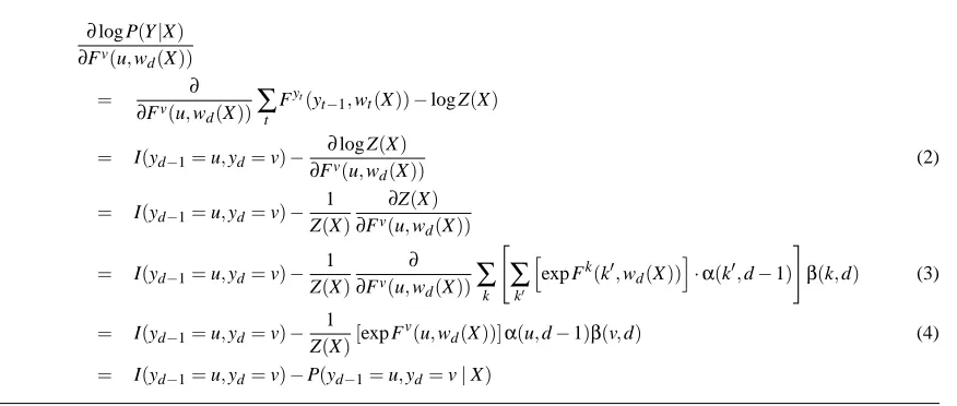
Proposition 1 The functional gradient of log P(Y|X)with respect to Fv(u,wd(X))is

∂log P(Y|X) ∂Fv_(u,w

d(X))

=I(yd−1=u,yd=v)−P(yd−1=u,yd=v|wd(X)) ,

where I(yd−1=u,yd=v)is 1 if the transition u→v is observed from position d−1 to position d in

the sequence Y and 0 otherwise, and where P(yd−1=u,yd=v|wd(X))is the predicted probability

of this transition according to the current potential functions.

To demonstrate this proposition, we must first introduce the forward-backward algorithm for computing the normalizing constant Z(X). We will assume that yt takes the value ⊥ for t <1.

Define the forward recursion by

α(k,1) = exp Fk(⊥,w1(X))

α(k,t) =

∑

k0

exp Fk(k0,wt(X))·α(k0,t−1) ,

and the backward recursion by

β(k,T) = 1

β(k,t) =

∑

k0

exp Fk0(k,wt+1(X))·β(k0,t+1) .

The variables k and k0 iterate over the possible class labels. The normalizer Z(X)can be computed at any position t as

Z(X) =

∑

α(k,t)β(k,t) .

If we unroll theαrecursion one step, we can also write this as

Z(X) =

∑

"

∑

k0

α(k0,t−1)·hexp Fk(k0,wt(X))

i #

β(k,t) .

Table 2 shows the derivation of the functional gradient. In Equation 2, exactly one of the Fyt_(y

t−1,wt(X)) terms will match Fv(u,wd(X)), because wd(X) is unique. This term will have

a derivative of 1, so we represent this by the indicator function I(yd−1=u,yd=v). In Equation 3,

we expand Z(X) at position d using the forward-backward algorithm. Again because wd(X) is

unique, only the product where k0 =u and k=v will give a non-zero derivative, so this gives us Equation 4. The right-hand expression in Equation 4 is precisely the joint probability that yd−1=u and yd=v given X . Q.E.D.

If wd(X)occurs more than once in X , each match contributes separately to the functional

gradi-ent.

∂log P(Y|X)

∂Fv_(u,w

d(X))

= ∂

∂Fv_(u,w

d(X))

∑

t−1,wt(X))−log Z(X)

= I(yd−1=u,yd=v)− ∂ log Z(X)

∂Fv_(u,w

d(X))

(2)

= I(yd−1=u,yd=v)− 1 Z(X)

∂Z(X)

∂Fv_(u,w

d(X))

= I(yd−1=u,yd=v)− 1 Z(X)

∂

∂Fv_(u,w

d(X))

∑

"

∑

k0

h

exp Fk(k0,wd(X))

i

·α(k0,d−1) #

β(k,d) (3)

= I(yd−1=u,yd=v)− 1 Z(X)[exp F

v_(u,w

d(X))]α(u,d−1)β(v,d) (4)

= I(yd−1=u,yd=v)−P(yd−1=u,yd=v|X)

Table 2: Derivation of the functional gradient.

should be 1 in order to maximize the likelihood. If the transition is not observed, then the predicted probability should be 0. Functional gradient ascent simply involves fitting regression trees to these residuals.

The pseudo code for our gradient tree boosting algorithm is shown in Table 3. The potential function for each class k is initialized to zero. Then M iterations of boosting are executed. In each iteration, for each class k, a set S(k) of functional gradient training examples is generated. Each example consists of a window wt(Xi)on the input sequence, a possible class label k0 at time t−1,

and the target∆value. A regression tree having at most L leaves is fit to these training examples to produce the function hm(k). This function is then added to the previous potential function to

produce the next function. In other words, we are setting the step sizeηm=1. We experimented

with performing a line search at this point to optimizeηm, but this is very expensive. So we rely on

the “self-correcting” property of tree boosting to correct any overshoot or undershoot on the next iteration.

The sets of generated examples S(k)can become very large. For example, if we have 3 classes and 100 training sequences of length 200, then the number of training examples for each class k is 3×100×200=60,000. Although regression tree algorithms are very fast, they still must consider all of the training examples! Friedman (2001) suggests two tricks for speeding up the computation: sampling and influence trimming. In sampling, a random sample of the training data is used for training. In influence trimming, data points with ∆values close to zero are ignored. We did not apply either of these techniques in our experiments.

TREEBOOST(Data,L)

// Data={(Xi,Yi): i=1, . . . ,N}

for each class k, initialize F₀k(·,·) =0 for m=1, . . . ,M

for class k from 1 to K

S(k):=GENERATEEXAMPLES(k,Data,Potm−1)

// where Potm−1={F_mu₋₁: u=1, . . .K}) hm(k):=FITREGRESSIONTREE(S(k),L)

F_mk:=F_mk₋₁+hm(k)

end end

return F_Mk for all k end TREEBOOST

GENERATEEXAMPLES(k,Data,Potm)

S :={}

for example i from 1 to N

execute the forward-backward algorithm on(Xi,Yi)

to getα(k,t)andβ(k,t)for all k and t for t from 1 to Ti

for k0from 1 to K

P(yi,t−1=k0,yi,t=k|Xi):=

α(k0,t−1)exp[F_mk(k0,wt(Xi))]β(k,t)

Z(Xi)

∆(k,k0,i,t):=I(yi,t−1=k0,yi,t =k)−

P(yi,t−1=k0,yi,t =k|Xi)

insert((wt(Xi),k0),∆(k,k0,i,t))into S

end end end return S

end GENERATEEXAMPLES

Table 3: Gradient tree boosting algorithm for CRFs.

5. Inference in CRFs

Once a CRF model has been trained, there are (at least) two possible ways to define a classifier Y =H(X)for making predictions. First, we can predict the entire sequence Y that has the highest probability:

H(X) =argmax

Y

This makes sense in applications, such as part-of-speech tagging, where the goal is to make a co-herent sequential prediction. This can be computed by the Viterbi algorithm (Rabiner, 1989), which has the advantage that it does not need to compute the normalizer Z(X).

The second way to make predictions is to individually predict each yt according to

Ht(X) =argmax v

P(yt=v|X) ,

and then concatenate these individual predictions to obtain H(X). This makes sense in applications where the goal is to maximize the number of individual yt’s correctly predicted, even if the resulting

predicted sequence Y is incoherent. For example, a predicted sequence of parts of speech might not be grammatically legal, and yet it might maximize the number of individual words correctly classified. P(yt|X)can be computed by executing the forward-backward algorithm as

P(yt|X) =

α(yt,t)β(yt,t)

Z(X) .

6. Handling Missing Values in CRFs with Gradient Tree Boosting

In some problem settings (e.g., activity recognition, sensor networks), the problem of missing values in the inputs can arise. The values of input features can be missing for a wide variety of reasons. Sensors may break or the sensor data feed may be lost or corrupted. Alternatively, input observations may not have been measured in all cases because, for example, they are expensive to obtain. Many methods for handling missing values have been developed for standard supervised learning, but many of them have not been tested on SSL problems. Recently, Sutton et al. (2006) used feature bagging method to deal with SSL problems where highly indicative features may be missing in the test data. A single CRF trained on all the features will be less robust, because the weights of weaker features will be undertrained. Feature bagging method divides all the original features into a collection of complementary and possibly overlapped feature subsets. Separate CRFs are trained on each subset and then combined.

With gradient tree boosting, a CRF is represented as a forest of regression trees. There exist very good methods for handing missing values when growing regression trees, which include instance weighting method of C4.5 (Quinlan, 1993) and surrogate splitting of CART (Breiman et al., 1984). An advantage of training CRFs with gradient tree boosting is that these missing values methods can be used directly in the process of generating regression trees over the functional gradient training examples.

6.1 Instance Weighting

The instance weighting method (Quinlan, 1993), also known as “proportional distribution”, assigns a weight to each training example, and all splitting decisions are based on weighted statistics. Ini-tially, each example has a weight of 1.0. When selecting a feature to split on, each boolean feature xj is evaluated based on the expected weighted squared error of the split using only the training

examples for which xjis not missing. The best feature xj∗is chosen, and the training examples for which xj∗is not missing are sent to the appropriate child node. Suppose that nle f texamples are sent

to the left child and nright examples are sent to the right child. The remaining training examples

of each example sent to the left child is multiplied by nle f t/(nle f t+nright). Similarly, the weight of

each example sent to the right child is multiplied by nright/(nle f t+nright).

At test time, when the test example reaches the test on feature xj∗, if the feature value is present, then the example is routed left or right in the usual way. But if xj∗is missing, then the example is sent to both children (recursively). Let ˆyle f tbe the predicted value computed by the left subtree and

ˆ

yright be the predicted value computed by the right subtree. Then the value predicted by node j∗is

the weighted average of these predictions:

ˆ

y=nle f tyˆle f t+nrightyˆright

nle f t+nright

.

Instance weighting assumes that the training and test examples missing xj∗will on average behave exactly like the training examples for which xj∗is not missing.

6.2 Surrogate Splitting

The surrogate splitting method (Breiman et al., 1984) involves separate procedures during training and testing. During training, as the regression tree is being constructed (in the usual top-down, greedy way), the key step in the learning algorithm is to choose which feature to split on. Each boolean feature xj is evaluated based only on the training examples that have non-missing values

for that feature, and the best feature, xj∗ is chosen. Each of the remaining features j06= j∗is then evaluated to determine how accurately it can predict the value of xj∗, and the features are sorted

according to their predictive power. This sorted list of features, called the surrogate splits, is stored in the node.

At test time, when test example x is processed through the regression tree, if xj∗is not missing, then the example is processed as usual by sending it to the left child if xj∗ is false and to the right child if xj∗ is true. However if xj∗ is missing, then surrogate split features are examined in order until a feature j0is found that is not missing. The value of this feature determines whether to branch left or right.

7. Experimental Results

We implemented gradient tree boosting algorithm for CRFs and compared it to McCallum’s Mal-let system (McCallum, 2002) on several data sets. We call our algorithm TREECRF. We use TREECRF-FB for the TREECRF with forward-backward predictions and TREECRF-V for the TREECRF with Viterbi predictions. MALLETdenotes the Mallet package with McCallum’s feature induction algorithm (McCallum, 2003) turned on. Similarly, we use MALLET-FB and MALLET-V for the MALLETwith forward-backward predictions and Viterbi predictions respectively. We also used the Mallet package to train standard CRFs without feature induction. We call it BASELINE, which serves as the baseline method. As before, BASELINE-FB donotes BASELINEwith forward-backward predictions and BASELINE-V denotes BASELINE with Viterbi predictions. Note that

MALLET-FB algorithm and BASELINE-FB algorithm are not implemented in the original Mallet

package. Instead we implemented them ourselves.

additional parameter is either the maximum number of leaves L in the regression trees using the best-first version of CART, or the regularization constantλfor the shrinkage alternative. For MALLET, the parameters are (a) the regularization penalty for squared weights (called the variance), (b) the number of iterations between feature inductions (kept constant at 8), (c) the number of features to add per feature induction (kept constant at 500), (d) the true label probability threshold (kept constant at 0.95), (e) the training proportions (kept constant at 0.2, 0.5, and 0.8). For BASELINE, the only additional parameter is the variance as in MALLET. Except for the variance, we kept all of MALLET’s parameters fixed at the values recommended by Andrew McCallum (personal communication). We did not optimize the window size, but instead employed values that have been used in previous studies. The chosen sizes are given in the following section. To set the remaining parameters, we manually tried the following settings and chose the setting that gave the best internal cross-validation performance:

• Number of leaves in regression trees: 30, 50, 75, 100, • TreeCRF regularization constant: 0, 5, 10, 20, 40, 80, • Weight variance prior in Mallet package: 1, 5, 10, 20.

Throughout the experiments, we measured the performance by computing the prediction accu-racy of individual labels, rather than individual sequences. McNemar’s test is employed to assess the statistical significance of these results.

7.1 Data Sets

Protein Secondary Structure Benchmark (Qian and Sejnowski, 1988). Each observation se-quence is a string of amino acid residues, and the corresponding output sese-quence is a string over the 3-letter alphabet{α,β,γ}, whereαindicates alpha helix,βindicates a beta sheet or beta turn, and

γindicates all other secondary structure types. There are 20 possible amino acid residues, and we represent each residue by a set of 20 indicator variables. There is a training set of 111 sequences and a test set of 17 sequences. An 11-residue sliding window is used in our experiments.

NETtalk Data Set. The original NETtalk task (Sejnowski and Rosenberg, 1987) is to assign a combination of phoneme and stress to each letter of the word so that the word is pronounced correctly. However, there are 140 legal phone-stress combinations, which gives a very large label space. Neither TREECRF nor MALLETis sufficient enough to work with such a large label space. Hence, we chose to study only the problem of assigning one of five possible stress labels to each letter. The labels are ‘2’ (strong stress), ‘1’ (medium stress), ‘0’ (light stress), ’<’ (unstressed consonant, center of syllable to the left), and ‘>’ (unstressed consonant, center of syllable to the right).

Each input sequence is an English word, a string of letters over the 26 letter alphabet. Each input observation is represented by 26 boolean indicator variables. There are 1000 training words and 1000 test words in our standard training and test sets. We employed a window size of 13 (window width of 6).

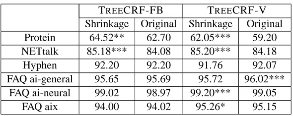
TREECRF-FB TREECRF-V Shrinkage Original Shrinkage Original Protein 64.52** 62.70 62.05*** 59.20 NETtalk 85.18*** 84.08 85.20*** 84.18

Hyphen 92.20 92.20 91.76 92.07

FAQ ai-general 95.65 95.69 95.72 96.02*** FAQ ai-neural 99.02 98.97 99.20*** 99.05

FAQ aix 94.00 94.02 95.26* 95.15

Table 4: Performance comparison of TREECRF with different regression tree fitting algorithms. En-tries marked with one or more stars are statistically significantly better than the alternative method. Specifically, * means p<0.025, ** means p<0.005 and *** means p<0.001 according to Mc-Nemar’s test.

letter. We manually constructed a training set of 1951 words and a test set of 908 words. The input window size is set to be 6 (i.e., 3 letters on either side of the potential hyphen location).

Usenet FAQs Data Sets. Each of the FAQ data sets consists of Frequently Asked Questions files for a Usenet newsgroup (McCallum et al., 2000). The FAQs for each newsgroup are divided in separate files: ai-general has 7 files, ai-neural has 7 files, and aix has 5 files. Every line of an FAQ file is labeled as either part of the header, a question, an answer, or part of the tail. Hence, each xt consists of a line in the FAQ file, and the corresponding yt ∈ {header, question, answer, tail}.

The measure of accuracy is the number of individual lines correctly classified. McCallum provided us with the definitions of 20 features for each line xt. We made a slight correction to one of the

features, so our results are not directly comparable to his. The size of the sliding window used here is 1. For each newsgroup, performance was measured by leave-1-out cross-validation: the CRF was trained on all-but-one of the files and tested on the remaining file. This was repeated with each file, and the results averaged.

7.2 Performance of Shrinkage in Regression Tree Generation

To evaluate the effectiveness of shrinkage in the regression tree fitting algorithm, we fixed L, the maximum number of leaves in regression trees, to be 100, and applied internal cross-validation to choose the best regularization constantλ. For purposes of comparison, we also implemented the original best-first regression tree generation algorithm. Internal cross-validation was employed to select the best value for L.

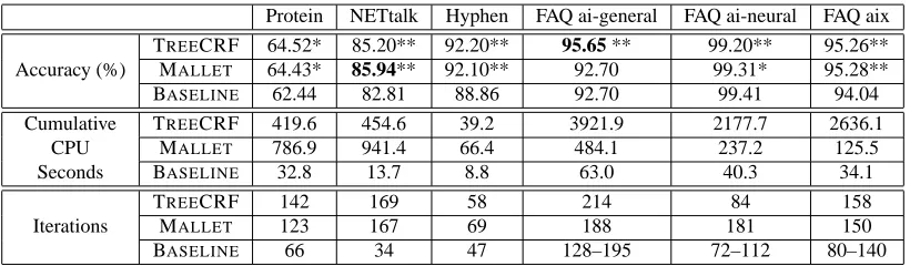
Protein NETtalk Hyphen FAQ ai-general FAQ ai-neural FAQ aix

TREECRF 64.52* 85.20** 92.20** 95.65 ** 99.20** 95.26**

Accuracy (%) MALLET 64.43* 85.94** 92.10** 92.70 99.31* 95.28**

BASELINE 62.44 82.81 88.86 92.70 99.41 94.04

Cumulative TREECRF 419.6 454.6 39.2 3921.9 2177.7 2636.1

CPU MALLET 786.9 941.4 66.4 484.1 237.2 125.5

Seconds BASELINE 32.8 13.7 8.8 63.0 40.3 34.1

TREECRF 142 169 58 214 84 158

Iterations MALLET 123 167 69 188 181 150

BASELINE 66 34 47 128–195 72–112 80–140

Table 5: Performance of TREECRF, MALLET, and BASELINE on each data set. Entries marked with one or more stars are statistically significant than BASELINE. Specifically, * means p<0.005, ** means p<0.001 according to McNemar’s test. Bolded numbers indicate the statistically better prediction accuracy between TREECRF and MALLET. The BASELINEmethod stops training if the optimization of loss functions converges. So for each FAQ data set, different training set may have different number of training iterations. Here we gave out the range of number of training iterations for each FAQ data set.

7.3 Comparison between TREECRF and MALLET

TREECRF and MALLET are the two leading CRF training methods that have feature induction capability. Here we compare the prediction accuracy and training speed of these two methods on each available data set. We also compare TREECRF and MALLET with the BASELINE method. For each method, internal cross-validation is applied to select the parameters that give the best performance of both forward-backward predictions and Viterbi predictions. The results reported here for each method are based on the prediction algorithm that gives higher prediction accuracy. All experiments were run on machines with 2.4 GHz Intel Xeon processors, 512KB cache, and 4GB memory.

Prediction Accuracy. Table 5 summarizes the prediction accuracy of TREECRF, MALLET, and BASELINEon each data set. McNemar’s tests show that on four of the data sets, that is, protein, hyphen, FAQ ai-neural and FAQ aix, the difference between the prediction accuracy of TREECRF and MALLETis not statistically significant. On the FAQ ai-general data set, the prediction accuracy of TREECRF is statistically better than that of MALLET(p<0.001). Only on the NETtalk data set is the prediction accuracy of MALLETstatistically better than that of TREECRF (p<0.05). In com-parison with the baseline method, the prediction accuracy of TREECRF and MALLETis statistically better than that of BASELINEin most cases. On the FAQ ai-general data set, the difference between

MALLETand BASELINE is not statistically significant. Only on the FAQ ai-neural data set is the

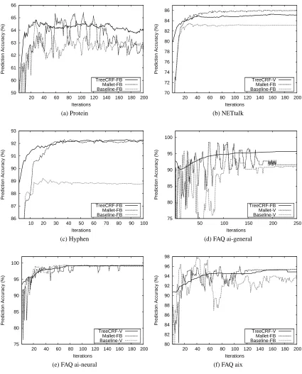
prediction accuracy of BASELINEstatistically better than that of both TREECRF and MALLET. Figure 1 plots the prediction accuracy of TREECRF, MALLETand BASELINEas a function of the number of training iterations. One worrying aspect of MALLETis that the performance curve exhibits a high degree of fluctuation, which is clearly shown on Figure 1a, 1d, 1e and 1f. This is presumably due to the effect of introducing new features. But it also suggests that it will be difficult to find the optimal stopping points for avoiding overfitting.

59 60 61 62 63 64 65 66

20 40 60 80 100 120 140 160 180 200

Prediction Accuracy (%)

Iterations TreeCRF-FB Mallet-FB Baseline-FB (a) Protein 70 72 74 76 78 80 82 84 86

20 40 60 80 100 120 140 160 180 200

Prediction Accuracy (%)

Iterations TreeCRF-V Mallet-FB Baseline-FB (b) NETtalk 86 87 88 89 90 91 92 93

10 20 30 40 50 60 70 80 90 100

Prediction Accuracy (%)

Iterations TreeCRF-FB Mallet-FB Baseline-FB (c) Hyphen 75 80 85 90 95 100

50 100 150 200 250

Prediction Accuracy (%)

Iterations

TreeCRF-FB Mallet-V Baseline-V

(d) FAQ ai-general

75 80 85 90 95 100

20 40 60 80 100 120 140 160 180 200

Prediction Accuracy (%)

Iterations

TreeCRF-V Mallet-FB Baseline-V

(e) FAQ ai-neural

80 82 84 86 88 90 92 94 96 98

20 40 60 80 100 120 140 160 180 200

Prediction Accuracy (%)

Iterations

TreeCRF-V Mallet-FB Baseline-FB

(f) FAQ aix

0 200 400 600 800 1000 1200

20 40 60 80 100 120 140 160 180 200

Cumulative CPU Seconds

Iterations TreeCRF-FB Mallet-FB Baseline-FB (a) Protein 0 200 400 600 800 1000 1200 1400 1600

20 40 60 80 100 120 140 160 180 200

Cumulative CPU Seconds

Iterations TreeCRF-V Mallet-FB Baseline-FB (b) NETtalk 0 10 20 30 40 50 60 70 80 90 100

10 20 30 40 50 60 70 80 90 100

Cumulative CPU Seconds

Iterations TreeCRF-FB Mallet-FB Baseline-FB (c) Hyphen 0 500 1000 1500 2000 2500 3000 3500 4000 4500 5000

50 100 150 200 250

Cumulative CPU Seconds

Iterations TreeCRF-FB

Mallet-V Baseline-V

(d) FAQ ai-general

0 1000 2000 3000 4000 5000 6000

20 40 60 80 100 120 140 160 180 200

Cumulative CPU Seconds

Iterations TreeCRF-V

Mallet-FB Baseline-V

(e) FAQ ai-neural

0 500 1000 1500 2000 2500 3000 3500

20 40 60 80 100 120 140 160 180 200

Cumulative CPU Seconds

Iterations TreeCRF-V

Mallet-FB Baseline-FB

(f) FAQ aix

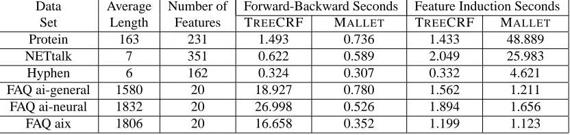
Data Average Number of Forward-Backward Seconds Feature Induction Seconds Set Length Features TREECRF MALLET TREECRF MALLET

Protein 163 231 1.493 0.736 1.433 48.889

NETtalk 7 351 0.622 0.589 2.049 25.983

Hyphen 6 162 0.324 0.307 0.332 4.621

FAQ ai-general 1580 20 18.927 0.780 1.562 1.211

FAQ ai-neural 1832 20 26.998 0.526 1.894 1.656

FAQ aix 1806 20 16.658 0.352 1.199 1.123

Table 6: Comparison of average CPU seconds spent per iteration on forward-backward algorithm and feature induction algorithm in TREECRF and MALLETfor each data set.

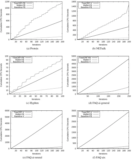
on different data sets can still give us some insight into the properties of these two methods. Figure 2 shows the number of cumulative CPU seconds consumed by these two methods on each data set. First, we can see that TREECRF scales linearly in the number of training iterations, because the cumulative CPU time has a constant slope. This makes sense, because for each potential function, only one regression tree is generated in each training iteration. Regression tree evaluations from previous iterations are cached so that they do not need to be re-evaluated. Without caching, the cumulative CPU curves for TREECRF would rise quadratically. Second, as shown in Figure 2a, 2b and 2c, TREECRF runs faster than MALLETon protein, NETtalk and hyphen data sets. But it is much slower than MALLETon FAQ data sets as shown in Figure 2d, 2e and 2f. The actual time required for each method to reach its peak performance on each data set is given in Table 5. Again we see that on the protein, NETtalk, and hyphen data sets, the time required for MALLETto reach its peak performance is about twice that of TREECRF. However, on the FAQ data sets, the time required for TREECRF to reach its peak performance is about 10-20 times more than for MALLET.

BASELINEis faster than both TREECRF and MALLETas shown in Figure 2 and Table 5.

Analysis and Discussion. We can explain the training speed difference between TREECRF and

MALLETby examining the details of these two methods. In both of them, most of the CPU time is

spent on two major computations: forward-backward inference and feature induction/tree growing. The relative proportion of these two computations varies from problem to problem. To measure this, we instrumented both TREECRF and MALLETto track the amount of CPU time spent on each of these two computations. Table 6 shows that on domains with short sequences (Protein, NETtalk, and Hyphen), the time spent by both algorithms on forward-backward inference is about the same. But for domains with very long sequences, TREECRF consumes much more CPU time in forward-backward inference. Conversely, in domains with a small number of basic features (the FAQ data sets), the two methods consume roughly the same amount of CPU time in feature induction. But in domains with a large number of basic features, TREECRF is much more efficient than MALLET.

prod-ucts are easier to compute than tree evaluations, but also possibly because of the reduced memory locality of regression trees.

Why would feature induction be more expensive in MALLET? In each feature induction it-eration, MALLETconsiders conjoining all of the basic features to each of the existing compound features. Hence, if there are n basic features and C compound features, this costs nC. Furthermore, C grows over time, so the cost of feature induction gradually increases. In the cumulative CPU time plots of Figure 2, the “steps’ in the “staircase” correspond to the feature induction iterations. In TREECRF, the cost of feature induction is the cost of growing a regression tree, which depends on the number of basic features n and the number of internal nodes in the tree L. This cost is nL, which remains constant across the iterations.

To verify our conjectures about the computational complexity of TREECRF and MALLET, we generated synthetic training data sets using a hidden Markov model (HMM) with 3 labels{l1,l2,l3} and 24 possible observations{o1, . . . ,o24}. To specify the observation distribution, for each label li,

we randomly draw an observation from the set{oi∗8−7, . . . ,oi∗8}with probability 0.6 and randomly draw an observation from the complement of this set with probability 0.4. The transition distribution is defined as P(yt =li|yt−1=li) =0.6 and P(yt=lj|yt−1=li) =0.2 if i6= j.

In order to measure the complexity of the forward-backward algorithm, we tried sequence lengths of 10, 20, 40, 80, 160 and 320. For each sequence length, we generated a training data set with 100 sequences and employed a sliding window of size 3. TREECRF and MALLETare run on each of these training data sets. Figure 3a shows the average CPU seconds spent per iteration on the forward-backward algorithm by these two methods. We see that the forward-backward algo-rithm in TREECRF implementation scales faster than that in MALLETimplementation as the length of sequence increases.

In order to measure the complexity of the feature induction algorithms, we generated a training data set with 100 sequences. The length of each sequences is 100. We tried sliding window sizes of 3, 5, 7, 9 and 11, so that the number of input features at each sequence position takes the values of 75, 125, 175, 225 and 275 (because each input observation is represented by 25 boolean indicator variables). TREECRF and MALLETare run for each sliding window size. Figure 3b shows the average CPU seconds spent per iteration on the feature induction algorithm by these two methods. It is clear that the feature induction algorithm in MALLETspends more and more CPU time than that in TREECRF as the number of basic features increases. In all the experiments on synthetic data sets, TREECRF uses regression trees of maximum 100 leaves and shrinkage constant 40. MALLET uses weight variance prior 20.

This analysis suggests that the performance of TREECRF could be improved by “flattening” the ensemble of regression trees to compute the corresponding vector of features and vector of weights. Then the cost of potential function evaluations would be similar to that of MALLET, and we would have a method that was faster than both the current TREECRF and MALLETimplementations.

7.4 Experimental Studies of Missing Values in TREECRF

We performed a series of experiments to evaluate the effectiveness of methods for handling missing values in TREECRF algorithm. In addition to the instance weighting and surrogate splitting methods described above, we also studied two simpler methods: imputation and indicator features. Let xt j,j=1, . . . ,n be the input features describing a particular input observation xt. Imputation and

0 0.5 1 1.5 2 2.5 3 3.5

10 20 40 80 160 320

CPU Seconds

Length of Sequence TreeCRF

Mallet

(a) Forward-backward algorithm

0 5 10 15 20 25

75 125 175 225 275

CPU Seconds

Number of Basic Features TreeCRF

Mallet

(b) Feature induction algorithm

Figure 3: Comparison of average CPU seconds spent per iteration on forward-backward algorithms and feature induction algorithms by TREECRF and MALLET.

Imputation: when a feature value xt j is missing, it is replaced with the most common value for

xj in the training data among those feature values that are not missing. This strategy can be

viewed as substituting the most likely value of xj a priori or alternatively as substituting the

value of xjleast likely to be informative.

Indicator Features: a boolean feature ˜xt j is introduced for each feature xt j such that if xt j is

present, ˜xt j is false. But if xt j is missing, then ˜xt j is true and xt j is set to a fixed chosen

value, typically 0. Indicator features make sense when the fact that a value is missing is itself informative. For example, if xt j represents a temperature reading, it may be that extremely

cold temperature values tend to be missing because of sensor failure.

We adopted a first-order Markov model in all the following experiments and employed an in-ternal hold-out method to set the other parameters: Two-thirds of the original training set was used as sub-training set and the other one third was used as development set to choose parameter values. Final training was performed using the entire training set.

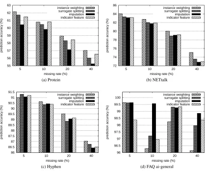
For each learning problem, we took the chosen training and test sets and inject missing values at rates of 5%, 10%, 20% and 40%. For a given missing rate, we generate five versions of the training set and five versions of the test set. A CRF is then trained on each of the training sets and evaluated on each of the test sets (for a total of 5 CRFs and 25 evaluations per missing rate). The label sequences are predicted by the forward-backward algorithm (i.e., we compute ˆyt=argmaxytP(yt|X) for each t separately). Prediction accuracy is based on the number of individual labels correctly predicted in the label sequences. The final prediction accuracy is the average of all 25 cases.

To test the statistical significance of the differences among the four methods, we performed an analysis of deviance based on the generalized linear model discussed by Agresti (1996). We fit a logistic regression model

log P(yt=yˆt) 1−P(yt =yˆt)

=δ1m1+δ2m2+δ3m3+

∑

55 56 57 58 59 60 61 62 63

5 10 20 40

prediction accuracy (%)

missing rate (%) instance weighting surrogate splitting imputation indicator feature (a) Protein 72 74 76 78 80 82 84 86

5 10 20 40

prediction accuracy (%)

missing rate (%) instance weighting surrogate splitting imputation indicator feature (b) NETtalk 86 86.5 87 87.5 88 88.5 89 89.5 90 90.5 91 91.5

5 10 20 40

prediction accuracy (%)

missing rate (%) instance weighting surrogate splitting imputation indicator feature (c) Hyphen 96 96.5 97 97.5 98 98.5 99 99.5 100

5 10 20 40

prediction accuracy (%)

missing rate (%) instance weighting

surrogate splitting imputation indicator feature

(d) FAQ ai-general

Figure 4: Performance of missing values methods for different missing rates.

where m1, m2, and m3are boolean indicator variables that specify which missing values method we are using and the S`’s are indicator variables that specify which of the five training sets we are using. If m1=m2=m3=0, then we are using instance weighting, which serves as our baseline method. If m1=1, this indicates surrogate splitting, m2=1 indicates imputation, and m3=1 indicates the indicator feature method. Consequently, the fitted coefficientsδ1,δ2, andδ3indicate the change in log odds (relative to the baseline) resulting from using each of these missing values methods. We can then test the hypothesisδi6=0 against the null hypothesisδi=0 to determine whether missing

values method i is different from the baseline method.

This statistical approach controls for variability due to the choice of the training set (through the

σ`’s) and variability due to the size of the test set.

Missing Surrogate Indicator

rate splitting Imputation feature

5% −0.018 −0.072* −0.028*

10% −0.013 −0.040* 0.001

20% −0.025* −0.074* −0.020*

40% −0.041* −0.072* −0.020*

(a) Protein

Missing Surrogate Indicator

rate splitting Imputation feature

5% −0.051* −0.066* −0.064*

10% −0.051* −0.067* −0.059*

20% −0.069* −0.057* −0.052*

40% −0.080* −0.116* −0.111*

(b) NETtalk

Missing Surrogate Indicator

rate splitting Imputation feature

5% 0.036* 0.007 0.023

10% −0.031* −0.022 −0.027*

20% −0.071* −0.049* −0.040*

40% −0.024* −0.054* −0.047*

(c) Hyphen

Missing Instance Surrogate Indicator

rate weighting splitting feature

5% −8.824E−16 −0.043 −1.499*

10% −2.161* −1.867* −1.961*

20% −0.874* 0.072 0.100

40% −1.243* −0.584* −0.359*

(d) FAQ ai-general

Table 7: Estimation of the coefficients corresponding to different missing values methods and statis-tical test results. In FAQ ai-general problem, imputation was the baseline method, so the coefficient values give the log odds of the change in accuracy relative to imputation. * means that the parameter value is statistically significantly different from zero (p<0.05).

NETtalk Stress Prediction. In Figure 4b, we see that instance weighting does better than the other three missing values methods for all the different missing rates. The statistical tests reported in Table 7b show that the baseline method, instance weighting, is statistically better than each of the other missing value methods in all cases.

Hyphenation. Figure 4c shows that instance weighting is the best missing values method except for a missing rate of 5%. Statistical tests shown in Table 7c tell us that for missing rate of 5%, surrogate splitting is the best missing values method and the other three methods are not statistically significantly different from each other. For a missing rate of 10%, instance weighting and imputation are statistically better than the other two methods (and indistinguishable from each other). For missing rates of 20% and 40%, instance weighting is statistically better than the other three methods. FAQ Document Segmentation. This task is based on the ai-general Usenet FAQ data set as we discussed before. We treat the first 6 files as the training set and the seventh file as the test set. The input window contains only the features corresponding to a single line in the file (window half-width of 0). Unlike in the previous data sets, instance weighting is no longer the best missing values method, as shown in Figure 4d. Instead, imputation performs very well for various missing value rates. Table 7d shows that imputation is statistically the best missing values method. For missing rates of 10% and 40%, it is statistically better than the other three methods. For a missing rate of 5%, it does as well as instance weighting and surrogate splitting. For a missing rate of 20%, it does as well as surrogate splitting and indicator features.

0 0.2 0.4 0.6 0.8 1

0 5 10 15 20

Fraction of time true

Feature Index

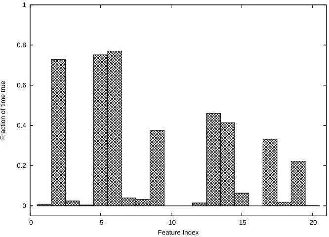
Figure 5: Fraction of the time that each FAQ feature is true (versus false). Features 1, 3, 4, 7, 8, 10, 11, 12, 16, 18, and 20 are rarely true.

tion sequence and setting all 20 boolean indicator features that represent that position to missing. Similarly, in the NETtalk and hyphenation problems, a letter is made to be missing by setting all 26 indicator features for that letter to missing. Similarly, imputation is computed at the amino acid or letter level, not at the level of boolean features. However, in the Usenet FAQ data set, since the bi-nary features are not exclusive, imputation is computed at the level of boolean features. In the case of protein sequences, imputation will replace missing values with the most frequently-occurring amino acid, which is alanine, code ‘A’. Alanine tends to form alpha helices, so this may cause the learning algorithms to over-predict the helix class, which may explain why imputation performed worst on the protein data set. In the case of English words, the most common letter is ‘E’, and it does not carry much information either about pronunciation or about hyphenation, so this may explain why imputation worked well in the NETtalk and hyphenation problems. Finally, in the ai-general FAQ data set, most of the features exhibit a highly skewed distribution, so that one feature value is much more common than another, as shown in Figure 5. Hence, in most cases, imputation with the most common feature value will supply the correct missing value. This may be why it worked best on that data set.

The surrogate splitting method assumes that the input features are correlated with one another, so that if one feature is missing, its value can be computed from another feature. The protein, NETtalk, and hyphenation data sets have a single input feature for each amino acid or letter. Hence, if this input feature is missing, then there is no information about that position in the sequence. The only exception to this would be if there were strong correlations between successive amino acids or letters. However, such strong correlations do not exist much either in protein sequences or in English, with the possible exception of the letter ‘q’, which is always followed by ‘u’. Note that the converse is not true: ‘u’ is not always preceded by ‘q’. Based on these considerations, we would not expect surrogate splitting to work well in these domains, and it does not.

In the FAQ data set, each line is described by 20 features computed from the words in that line. In the experiment, each of these 20 features could be independently marked as missing, which is a bit unrealistic, since presumably the real missing values would involve some loss or corruption of the words making up the line, and this would affect multiple features. The 20 features do have some redundancy, so we would expect that surrogate splitting should work well, and it does for 5% and 20% missing rates.

The instance weighting method assumes that the feature values are missing at random and that the other features provide no redundant information, so the most sensible thing to do is to marginal-ize away the uncertainty about the missing values. Our experiments show that this is a very good strategy in all cases except for the FAQ data set, where the features are somewhat redundant.

8. Conclusions

In this paper, we presented TREECRF, a novel method for training conditional random fields based on gradient tree boosting. TREECRF has the ability to construct very complex feature conjunctions from basic features and scales much better than methods based on iterative scaling and simple gradient descent. It appears to match the L-BFGS algorithm implemented in MALLET, which also gives dramatic speedups when there are many potential features. In our experiments, TREECRF is as accurate as MALLET on four data sets, more accurate on one data set and less accurate on one data set. Its feature induction method is faster than that of MALLETfor problems with a large number of features. But its forward-backward implementation is slower than that of MALLETfor really long sequences. In addition, TREECRF is easier to implement and tune. It introduces only one tunable parameter (either the maximum number of leaves permitted in each regression tree or the regularization constant), whereas MALLEThas many more parameters to consider. It is easier for the TREECRF to find the optimal stopping point to avoid overfitting, since its performance improves smoothly, while that of MALLETfluctuates wildly. Combining the benefit of these two methods will be a promising direction to pursue.

boosting. Since there is no one best method for handling missing values, as with many other aspects of machine learning, preliminary experiments on subsets of the training data are required to select the most appropriate method.

Acknowledgments

The authors would like to thank the anonymous reviewers and the action editor for their constructive input. We also gratefully acknowledge the support of NSF grants IIS-0083292 and IIS-0307592. Some of the material in this paper was first published at ICML-2004 (Dietterich et al., 2004).

References

Alan Agresti. An Introduction to Categorical Data Analysis. Wiley, New York, 1996.

Yasemin Altun, Ioannis Tsochantaridis, and Thomas Hofmann. Hidden markov support vector machines. In Tom Fawcett and Nina Mishra, editors, Proceedings of the 20th International Con-ference on Machine Learning (ICML 2003), pages 3–10. AAAI Press, 2003.

Julian Besag. Spatial interaction and the statistical analysis of lattice systems. Journal of the Royal Statistical Society B, 36(2):192–236, 1974.

Leo Breiman, Jerome H. Friedman, Richard A. Olshen, and Charles J. Stone. Classification and Regression Trees. Wadsworth Publishing Company, 1984.

Thomas G. Dietterich, Adam Ashenfelter, and Yaroslav Bulatov. Training conditional random fields via gradient tree boosting. In Proceedings of the 21st International Conference on Machine Learning (ICML 2004), pages 217–224, Banff, Canada, 2004. ACM Press.

Yoav Freund and Robert E. Schapire. Experiments with a new boosting algorithm. In Proceedings of the 13th International Conference on Machine Learning (ICML 1996), pages 148–156. Morgan Kaufmann, 1996.

Jerome Friedman. Greedy function approximation: A gradient boosting machine. The Annals of Statistics, 29(5):1189–1232, 2001.

Jerome Friedman, Trevor Hastie, and Robert Tibshirani. Additive logistic regression: a statistical view of boosting. The Annals of Statistics, 38(2):337–374, 2000.

Stuart Geman and Donald Geman. Stochastic relaxation, gibbs distributions, and the bayesian restoration of images. IEEE Transactions on Pattern Analysis and Machine Intelligence, 6(6): 721–741, Nov. 1984.

John M. Hammersley and Peter Clifford. Markov fields on finite graphs and lattices. Technical report, Unpublished, 1971.

Lin Liao, Tanzeem Choudhury, Dieter Fox, and Henry A. Kautz. Training conditional random fields using virtual evidence boosting. In Manuela M. Veloso, editor, Proceedings of the 20th Interna-tional Joint Conference on Artificial Intelligence (IJCAI 2007), pages 2530–2535, Hyderabad, India, January 6-12 2007.

Andrew McCallum. Efficiently inducing features of conditional random fields. In Christopher Meek and Uffe Kjaerulff, editors, Proceedings of the 19th Conference on Uncertainty in Artificial Intelligence (UAI 2003), pages 403–410. Morgan Kaufmann, 2003.

Andrew McCallum, Dayne Freitag, and Fernando C. N. Pereira. Maximum entropy markov models for information extraction and segmentation. In Proceedings of the 17th International Conference on Machine Learning (ICML 2000), pages 591–598. Morgan Kaufmann, 2000.

Andrew Kachites McCallum. Mallet: A machine learning for language toolkit. http://mallet.cs.umass.edu, 2002.

Andrew Y. Ng and Michael Jordan. On discriminative vs. generative classifiers: A comparison of logistic regression and naive Bayes. In Advances in Neural Information Processing Systems, volume 14. MIT Press, 2002.

Ning Qian and Terrence J. Sejnowski. Predicting the secondary structure of globular proteins using neural network models. Journal of Molecular Biology, 202:865–884, 1988.

J. Ross Quinlan. C4.5: Programs for Machine Learning. Morgan Kaufmann, San Francisco, CA, 1993.

Lawrence R. Rabiner. A tutorial on hidden markov models and selected applications in speech recognition. Proceedings of the IEEE, 77(2):257–286, 1989.

Adwait Ratnaparkhi. A maximum entropy model for part-of-speech tagging. In Eric Brill and Kenneth Church, editors, Proceedings of the Conference on Empirical Methods in Natural Lan-guage Processing, pages 133–142, Somerset, New Jersey, 1996. Association for Computational Linguistics.

Terrence J. Sejnowski and Charles R. Rosenberg. Parallel networks that learn to pronounce english text. Complex Systems, 1:145–168, 1987.

Fei Sha and Fernando Pereira. Shallow parsing with conditional random fields. In Marti Hearst and Mari Ostendorf, editors, HLT-NAACL 2003: Main Proceedings, pages 213–220, Edmonton, Alberta, Canada, May 27 – June 1 2003. Association for Computational Linguistics.

Charles Sutton, Michael Sindelar, and Andrew McCallum. Reducing weight undertraining in struc-tured discriminative learning. In Proceedings of the main conference on Human Language Tech-nology Conference of the North American Chapter of the Association of Computational Linguis-tics, pages 89–95, Morristown, NJ, USA, 2006. Association for Computational Linguistics.

Ioannis Tsochantaridis, Thomas Hofmann, Thorsten Joachims, and Yasemin Altun. Support vector machine learning for interdependent and structured output spaces. In Proceedings of the 21st International Conference on Machine Learning (ICML 2004), pages 823–830, Banff, Canada, 2004. ACM Press.