Students' understanding of statistical inference : implications for teaching

(1)

Students’ Understanding of Statistical

Inference: Implications for Teaching

by

Robyn Reaburn, B.App.Sci.(Medical Technology),

BA, Dip.Teach.,Grad.Dip.Sci.,MSc.

Submitted in fulfilment of the

requirements for the Degree of Doctor of

Philosophy

(2)

(3)

(4)

(5)

v Abstract

It was of concern to the researcher that students were successfully completing in-troductory tertiary statistics units (if success is measured by grades received), without having the ability to explain the principles behind statistical inference. In other words, students were applying procedural knowledge (surface learning) without concurrent conceptual knowledge.

This study had the aim of investigating if alternative teaching strategies could as-sist students in gaining the ability to explain the principles behind two tools of statistical inference: P-values and confidence intervals for the population mean. Computer simulations were used to introduce students to statistical concepts. Stu-dents were also introduced to alternative representations of hypothesis tests, and were encouraged to give written explanations of their reasoning. Time for reflec-tion, writing and discussion was also introduced into the lectures.

It was the contention of the researcher that students are unfamiliar with the hypo-thetical, probabilistic reasoning that statistical inference requires. Therefore stu-dents were introduced to this form of reasoning gradually throughout the teaching semester, starting with simple examples that the students could understand. It was hoped that by the use of these examples students could make connections that would form the basis of further understanding.

(6)

sim-vi ple examples were more difficult to find, student understanding did not improve to the extent that it did for P-values.

(7)

vii Acknowledgements

I would like to thank my supervisors, Professor Jane Watson and Associate Pro-fessor Kim Beswick, and my research supervisor, Associate ProPro-fessor Rosemary Callingham, for their help and support over the time of my candidature. They have been consistently helpful, cheerful, and encouraging. It has been my good fortune to work with them. Thanks also to Dr. Des Fitzgerald, coordinator of the statistics unit described in this study, for his advice.

I wish to thank my parents, Kenneth and Phyllis Duck. They did all they could so that their daughters could have the education that they could never have. My fa-ther died during the time this thesis was written; he would have been thrilled to know that it has been finished.

(8)

8

.

1. INTRODUCTION ... 15

1.1 WHY DO THIS RESEARCH? ... 15

1.2THE RESEARCH QUESTIONS ... 17

1.3A NOTE ON THE TERMINOLOGY ... 18

2. LITERATURE REVIEW – PART I: STATISTICAL REASONING ... 20

2.1WHAT IS STATISTICS? ... 20

2.2STATISTICAL REASONING ... 21

2.3HYPOTHESIS TESTING AND CONFIDENCE INTERVALS ... 22

2.3.1 Hypothesis testing ... 22

2.3.2 Confidence intervals ... 26

2.4MISCONCEPTIONS WITH PROBABILISTIC REASONING ... 28

2.4.1 Introduction ... 28

2.4.2 The contribution of Tversky and Kahneman ... 29

2.4.3 Other misconceptions about probability ... 32

2.4.4 Misconceptions about conditional probability ... 33

2.5OTHER MISCONCEPTIONS ABOUT STATISTICAL REASONING ... 34

2.5.1 Misconceptions about randomness ... 34

2.5.2 Misconceptions about sampling ... 35

2.5.3 Misconceptions about measures of central tendency ... 36

2.5.4 Misconceptions about statistical inference ... 38

2.6THE PERSISTENCE OF PRECONCEIVED VIEWS ... 47

2.6.2 How students change their previous conceptions ... 47

2.7IMPLICATIONS OF THE LITERATURE FOR TEACHING STATISTICS ... 48

3. LITERATURE REVIEW PART II: THE NATURE OF LEARNING ... 50

3.1INTRODUCTION -WHAT IS LEARNING? ... 50

3.2HOW LEARNING OCCURS ... 51

(9)

9

3.2.3 Constructivist theories of learning ... 53

3.2.4 Implications of the cognitive models for teaching ... 55

3.3AFFECTIVE FACTORS ... 56

3.4THE USE OF THE SOLO TAXONOMY IN ASSESSING LEARNING ... 58

4. LITERATURE REVIEW PART III: MEASUREMENT IN THE SOCIAL SCIENCES ... 60

4.1SCALES USED IN MEASUREMENT ... 60

4.2MEASUREMENT THEORY ... 62

4.3SHOULD THE SOCIAL SCIENCES USE MEASUREMENT? ... 66

4.4ITEM RESPONSE THEORY ... 67

4.5THE MATHEMATICS OF THE RASCH MODEL... 73

4.5.1 The Dichotomous model ... 73

4.5.2 The Partial Credit Model ... 75

4.5.3 How Rasch analysis was used in this study ... 78

5. THE USE OF COMPUTER TECHNOLOGY IN STATISTICS ... 83

EDUCATION ... 83

5.1 Introduction ... 83

5.2 Discovery Learning and Simulation ... 83

5.3 Simulation in statistics ... 85

5.4 How computers were used in this study ... 88

6. THE STUDY DESIGN ... 89

6.1INTRODUCTION ... 89

6.2RESEARCH DESIGNS IN EDUCATION ... 90

6.2.1 Scientific Research in Education... 91

6.2.2 How “Scientific” Does Knowledge Have To Be? ... 94

6.2.3 The Action Research Method of educational research ... 95

6.2.4 How this study fitted the research paradigms ... 97

6.3 THE STUDY – AIMS, PARTICIPANTS, TASKS, INTERVENTIONS ... 97

6.3.1 The aims of the study ... 97

6.3.2 The participants in the study ... 98

(10)

10

6.4THE DESIGN FOR THIS STUDY ... 107

6.4.2 The pre-intervention semester ... 108

6.4.3 The first cycle of the intervention ... 110

6.4.4 The second cycle of the intervention ... 114

6.4.5 The third cycle of the intervention ... 117

6.5 A SUMMARY OF THE STUDY DESIGN ... 120

6.6 CONSTRAINTS ON THE RESEARCH ... 122

7. RESULTS OF THE QUANTITATIVE AND QUALITATIVE ANALYSIS OF THE FIRST QUESTIONNAIRE ... 124

7.2RASCH ANALYSIS OF THE FIRST QUESTIONNAIRE ... 126

7.2.2 Items in the First Questionnaire ... 126

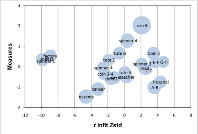
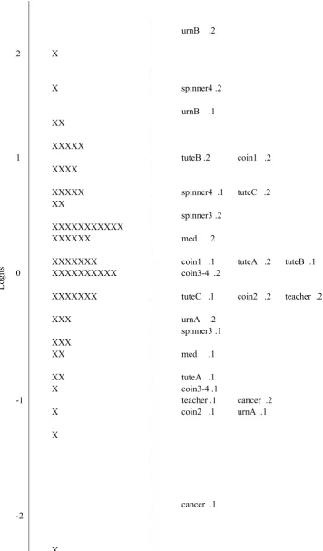
7.2.3 The Rasch Analysis of the Items (Partial Credit Model) ... 128

7.2.4 Rasch analysis of persons ... 137

7.3QUALITATIVE ANALYSIS OF THE FIRST QUESTIONNAIRE ... 140

7.3.1 Questions requiring interpretation of verbal probabilistic statements ... 140

7.3.2 Questions requiring an understanding of statistical independence ... 144

7.3.3 Students‟ Awareness of Variation in Stochastic Processes ... 151

7.3.4 Questions requiring judgements of differences between groups ... 161

7.3.5 Conditional probability questions ... 171

7.4SUMMARY AND DISCUSSION ... 176

8. RESULTS OF THE QUANTITATIVE AND QUALITATIVE ANALYSIS OF THE SECOND QUESTIONNAIRE ... 180

8.2.RASCH ANALYSIS OF THE SECOND QUESTIONNAIRE ... 181

8.2.2 Items in the Second Questionnaire ... 181

8.2.3 The Rasch Analysis of the Items (Partial Credit Model) ... 183

(11)

11

8.3QUALITATIVE ANALYSIS OF THE SECOND QUESTIONNAIRE ... 195

8.3.1 The circuit breaker questions ... 195

8.3.2 Explaining the meaning of “significant difference” ... 198

8.3.3 Judgement as to the likelihood of sample means, given a population mean ... 201

8.3.4 The Use of Informal Inference ... 207

8.3.5 Questions that deal with randomness – what is random, and why randomise? ... 209

8.3.6 Repeated questions from the first questionnaire ... 215

8.4RELATIONSHIPS AMONG ABILITY MEASURES AND SCORES FROM FORMAL ASSESSMENTS ... 222

8.5SUMMARY AND DISCUSSION ... 226

9. AN ANALYSIS OF STUDENTS’ UNDERSTANDING OF P-VALUES. ... 228

9.1.INTRODUCTION ... 228

9.2RESULTS OF THE PRE-INTERVENTION SEMESTER (SEMESTER 2–2007) ... 230

9.2.1 Teaching strategies ... 230

9.2.2 Student answers to the P-value items in the test ... 231

9.3 RESULTS OF THE FIRST CYCLE OF THE INTERVENTION (SEMESTER 1–2008) ... 232

9.4RESULTS OF THE SECOND CYCLE OF THE INTERVENTION (SEMESTER 2–2008) ... 234

9.4.2 Student answers ... 236

9.5 RESULTS OF THE THIRD CYCLE OF THE INTERVENTION (SEMESTER 1–2009) ... 237

9.6 A DESCRIPTION OF THE TEACHING STRATEGIES USED IN THE TEACHING OF P-VALUES IN SECOND CYCLE OF THE INTERVENTION ... 242

9.6.1 Stage 1 – Introduction to probabilistic reasoning ... 243

9.6.2 Stage 2 – Consolidation – hypothetical probabilistic reasoning in another context ... 246

9.6.3 Stage 3 – Simulation of P-values ... 247

(12)

12 9.6.5 Stage 5 – P-values in other contexts – chi-squared tests for independence, the analysis

of variance, and linear regression ... 255

9.6.6 Stage 6 - revision ... 260

9.7 SUMMARY OF THE MISCONCEPTIONS IDENTIFIED DURING THE STUDY IN COMPARISON TO THE LITERATURE ... 261

9.8 HOW STUDENTS‟ UNDERSTANDING CHANGED OVER THE INTERVENTION ... 262

9.9 IMPLICATIONS FOR TEACHING ... 264

10. AN ANALYSIS OF STUDENTS’ UNDERSTANDING OF CONFIDENCE INTERVALS . 267 10.1INTRODUCTION ... 267

10.2 RESULTS OF THE PRE-INTERVENTION SEMESTER (SEMESTER 2–2007) ... 270

10.2.2 Student answers to the confidence interval questions ... 271

10.3 RESULTS OF THE FIRST CYCLE OF THE INTERVENTION (SEMESTER 1–2008) ... 271

10.4 RESULTS OF THE SECOND CYCLE OF THE INTERVENTION (SEMESTER 2–2008) ... 274

10.5 RESULTS OF THE THIRD CYCLE OF THE INTERVENTION (SEMESTER 1–2009) ... 277

10.6 A DESCRIPTION OF THE TEACHING STRATEGIES USED IN THE TEACHING OF CONFIDENCE INTERVALS IN THE SECOND CYCLE OF THE INTERVENTION ... 280

10.6.1 Stage 1 – Introduction to the distribution of sample means ... 281

10.6.2 Stage 2 – Putting the information into a mathematical format ... 284

10.6.3 Stage 3 - Formal introduction to confidence intervals for the mean ... 288

10.6.4 Stage 4 – Practice and consolidation ... 290

10.6.5 Stage 5 – Responses to questions on part of the formal assessment ... 294

(13)

13

10.7SUMMARY OF THE MISCONCEPTIONS IDENTIFIED DURING THE STUDY IN COMPARISON TO

THE LITERATURE ... 297

10.8A SUMMARY OF STUDENTS‟ UNDERSTANDING OVER THE INTERVENTION ... 298

10.9 IMPLICATIONS FOR TEACHING ... 299

11. DISCUSSION WITH IMPLICATIONS FOR TEACHING... 302

What are students‟ understandings of probability and stochastic processes on entering university? Are there any differences in understandings between those students who have studied statistics in their previous mathematics courses and those who have not? ... 302

What are students‟ understandings of P-values at the end of their first tertiary statistics unit? How did these understandings change over the time of the study? ... 309

What are students‟ understandings of confidence intervals at the end of their first tertiary statistics unit? How did these understandings change over the time of the study? ... 314

Constraints on the research - suggestions for further research ... 317

12. A PERSONAL REFLECTION ... 319

REFERENCES ... 323

APPENDIX A: DETAILS OF THE DATA HANDLING AND STATISTICS UNIT - THE TRADITIONAL TEACHING PROGRAM WITH THE ADDITIONS FOR THE FIRST CYCLE OF THE INTERVENTION ... 340

APPENDIX B: THE QUESTIONNAIRES AND TEST QUESTIONS ... 348

B1 The first questionnaire ... 348

B2 The Second Questionnaire ... 359

B3 The Test Questions used in this study ... 368

APPENDIX C: THE CODING PROTOCOLS ... 369

C1 Coding protocol for the first questionnaire ... 369

C2 Coding protocol for the second questionnaire ... 372

C3 Coding protocols for the test items ... 374

APPENDIX D: THE SIMULATIONS AND DEMONSTRATIONS ... 375

D1 Introduction ... 375

D2 Introduction to simulation – the Chinese birth problem ... 375

D3 Demonstration – Means vs. Medians ... 376

D4 Simulation – What is “random”?... 378

(14)

14

D6 Simulation – the sampling distribution of the mean ... 382

D7 Simulation – hypothesis testing ... 387

D8 Demonstration/simulation – how confidence intervals work ... 389

D9 Simulation – The Grade 12 Heights problem ... 391

D10. Simulation – the chi-squared test for independence. ... 393

D11 Simulation – Fitting a line of best fit to data with measurement error ... 394

D12 Demonstration – The Analysis of Variance ... 398

APPENDIX E: STATISTICAL ANALYSES ... 400

E1 Analyses of the first questionnaire ... 400

E2 Analyses of the second questionnaire ... 405

E3 Comparisons between ability scores and final scores from formal assessment ... 408

E4. Comparison among semesters for the P-value and confidence interval questions on the

(15)

15

1. Introduction

1.1 Why do this research?

I have long felt that many students, although they can successfully follow the pro-cedure to carry out a hypothesis test, do not understand the reasoning behind this process. In particular, it appears that students find difficulty in explaining the rea-soning behind the P-values in hypothesis testing and in understanding that confi-dence intervals are used to estimate population parameters.

I, myself, was a successful undergraduate statistics student in that I received high grades. Looking back, however, I realise that although I was successfully follow-ing the process I would not have been able to explain the reasonfollow-ing behind confi-dence intervals and hypothesis tests.

I am now a lecturer of a first year statistics unit at a tertiary institution and I have found that when students are asked questions that require conceptual understand-ing (in contrast to procedure) they often demonstrate a lack of understandunderstand-ing. For example, in one assignment students are asked to calculate the confidence interval for a mean, and then in a separate question they are asked to calculate the interval where 95% of the individuals are expected to lie. These questions cause intense angst and confusion. It is apparent from their answers that the students often do not appreciate the difference between the questions.

(16)

-16 value that the population means may not be different from each other? It is appar-ent from the studappar-ent answers that the studappar-ents can successfully complete the process and conclude that the null hypothesis should be accepted. Many of them cannot, however, explain the role of sampling variation and what the P-value is in conceptual terms. It would appear that the students are using procedural knowl-edge only.

The literature indicates that my suspicion, that many students do not understand hypothesis testing, is also of concern to others. For example, Garfield (2002, p. 3) has found “that students can often do well in a statistics course, earning good grades on homework, exams and projects, yet still perform poorly on a measure of statistical reasoning such as the Statistical Reasoning Assessment.” Garfield and Ahlgren (1988) also report that students use procedural knowledge without understanding the concepts behind what they are doing:

The experience of most college faculty members in education and the social sciences is that a large proportion of university students in introductory statistics courses do not understand many of the concepts they are studying … Students often tend to respond to problems involving mathematics in general by falling into “number crunching” mode, plugging quantities into a computational formula or procedure without forming an in-ternal representation of that problem. (p. 46)

(17)

17

1.2 The Research Questions

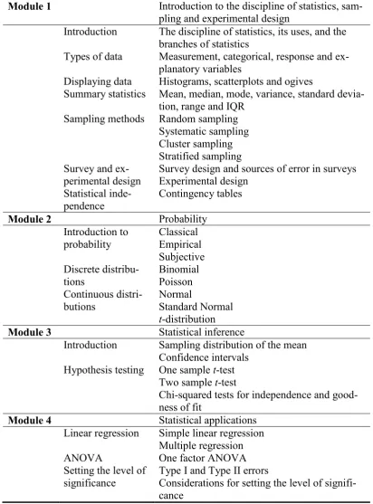
Before this research commenced the Data Handling and Statistics unit was taught in a didactic style and little attempt was made to discover the students‟ c oncep-tions before and during the unit. The unit was taught in four modules. The first module consisted of the summarisation of data and data collection methods. The second module introduced probability and probability distributions. The third module introduced confidence intervals and hypothesis testing. The final module introduced the Analysis of Variance (ANOVA) and simple and multiple linear regression. One consequence of the way the material was presented was that stu-dents had to grapple with the formal hypothesis testing procedures at the same time as they were introduced to hypothetical and probabilistic reasoning. They had little or no time to gather experience with drawing conclusions using prob-ability and to become familiar with hypothetical reasoning before the use of for-mal procedures.

With these factors in mind the research questions were:

 What are students‟ understandings of probability and stochastic processes on entering university? Are there any differences in understandings be-tween those students who have studied statistics in their previous mathe-matics courses and those who have not?

(18)

18

 What are students‟ understandings of confidence intervals at the end of their first tertiary statistics unit? How did these understandings change over the time of the study?

1.3 A note on the terminology

Students come into any learning environment with their own views of the world which they have gained over their life experience. These beliefs may be inconsis-tent with formal knowledge, that is, “inconsisinconsis-tent with commonly accepted and well-validated explanations of phenomena or events” (Ormrod, 2008, p. 245). In the educational literature views that are not consistent with formal knowledge, are referred to as “misconceptions,” “misunderstandings” or, in the more recent lit-erature, “alternative conceptions” (Sotos, Vanhoof, Van den Noortgate, & Onghena, 2007). In the literature pertaining to tertiary statistics education, how-ever, the term “misconceptions” is generally retained. Therefore this term is used for this study.

(19)

(20)

20

2. Literature Review – part I: Statistical Reasoning

2.1 What is statistics?

“Statistics is the science of collecting, organising, analysing, interpreting, and presenting data” (Doane & Seward, 2007, p. 3). In practice, statistics involves the use of numbers within a context and involves data collection, summarising these data in some way and making interpretations and decisions.

There are two general areas of statistics, descriptive statistics and inferential statistics. With descriptive statistics, data are summarised with graphs, tables and numbers such as means and standard deviations. Inferential statistics involves the making of conclusions about entire populations from samples (Doane & Seward, 2007). This latter field involves the use of probability and hypothetical reasoning. Because variation is universal, and no two samples are alike, no sample is likely to be exactly representative of the population from which it was drawn. The use of samples, therefore, always results in uncertainty concerning the accuracy of the conclusions inferred from samples.

(21)

21 are used to working towards a single “correct” answer in other branches of

mathematics the need to address these differences can be unexpected and discon-certing.

These differences have led some writers to look at statistics as being not a branch of mathematics at all. For example, Shaughnessy (2006, p. 78) states, “Statisti-cians are quite insistent that those of us who teach mathematics realise that statis-tics is not mathemastatis-tics, nor is it even a branch of mathemastatis-tics.”

The successful use of statistics, however, does require skills that are usually re-garded as mathematical. Not only does the discipline of statistics require the summary and interpretation of data with graphs and numbers such as the mean and median, it also requires hypothetical reasoning that in turn uses the mathemat-ics of probability. Common statistical procedures are based on what Cobb and Moore (1997, p. 803) refer to as “elaborate mathematical theories [and] the study of these theories is part of the training of statisticians.”

2.2 Statistical reasoning

(22)

22 sample puts limits on the estimated value of a characteristic of the population. That is, students need to be able to cope with the conflicting ideas that samples do not exactly represent a population but are in some way still representative of that population (Rubin, Hammerman, & Konold, 2006).

A result of the tension between the representativeness and variability of samples is that statistical inference leads to the formation of conclusions based on a hypo-thetical reasoning process (hypothesis testing), and which are stated in probabilis-tic terms. The result of the presence of variation leads the user of statisprobabilis-tics to an-swer the following question, “Is the observed effect larger than can be reasonably attributed to chance alone?” (Moore, 1990).

2.3 Hypothesis testing and confidence intervals

2.3.1 Hypothesis testing

What distinguishes science from other fields of knowledge? It was in the search for the answer to this question that Popper (1963) proposed the criterion of “falsi-fiability, or refutability, or testability” (p. 37). By this criterion, “statements or systems of statements, in order to be ranked as scientific, must be capable of con-flicting with possible, or conceivable observations” (p. 39). A “theory that is not refutable by any conceivable event is non-scientific” (p. 36).

This proposal, that scientific statements must be capable of being falsified, is sometimes introduced to students with reasoning similar to this. A statement is made such as:

(23)

23 It is not possible to prove this statement true. No matter how many white swans are observed, there is always the possibility that the next swan observed may not be white. In contrast, it is possible to disprove this statement by the observation of only one swan of another colour. Therefore, according to Popper‟s criterion of falsification, because the statement about swans is capable of being disproved, it is scientific.

Similar reasoning is used in statistical hypothesis testing. A proposition (the “null hypothesis”, designated H0) is made about a parameter (for example, the mean) of

(24)

exam-24 ple, if the hypothesis is about the value of a population mean, the probability would be expressed in mathematical terms as:

) |

) 0 |

((|x  H_o 

P

wherex is the mean of the sample, and µ is the mean of the population. If this probability is found to be very low, then it is concluded that evidence has been found against the null hypothesis and it is rejected. If this probability is not very low, then the hypothesis is accepted.

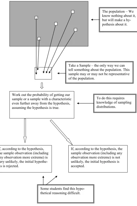
Lipson, Kokonis and Francis (2003) have summarised the reasoning involved in hypothesis testing as a stepwise process. The first step involves the recognition that no two samples are alike, even if they had been drawn from the same popula-tion. The second step involves comparing the sample result with that expected from the hypothesised population. To do this, a knowledge of sampling distribu-tions (the pattern into which the sample statistics from the hypothesised popula-tion would fall) is required. If the hypothesis should be rejected, then the next step involves recognition that there is an inconsistency between the sample and the hypothesised population, and that the sample may not belong to that of the hy-pothesised population.

(25)

[image:25.595.106.548.86.753.2]

25

Figure 2.3.1.1. Model of a hypothesis test.

The population – We know nothing about it, but will make a hy-pothesis about it.

Take a Sample – the only way we can tell something about the population. This sample may or may not be representative of the population.

Work out the probability of getting our sample or a sample with a characteristic even further away from the hypothesis, assuming the hypothesis is true.

To do this requires knowledge of sampling distributions.

If, according to the hypothesis, the sample observation (including any observation more extreme) is very unlikely, the initial hypothe-sis is rejected.

If, according to the hypothesis, the sample observation (including any observation more extreme) is not unlikely, the initial hypothesis is accepted.

(26)

26 In summary, successful hypothesis testing requires:

 An understanding of randomness and probability.

 An understanding of data collection and the recognition that samples may not be representative of the parent population.

 An understanding of what summary statistics such as the mean and stan-dard deviation represent, that is, an understanding that is more than just how these numbers are calculated.

 An understanding of how sample statistics such as the mean relate to the equivalent statistics in the population (in populations these statistics are known as parameters).

 An understanding that variation is omnipresent, and of the extent of varia-tion to be expected in the data.

 An understanding of the legitimate interpretations of hypothesis tests, in-cluding the setting up and correct interpretations of the null and alternative hypotheses, and correct interpretations of P-values and levels of signifi-cance.

These areas are discussed in turn in Sections 2.4 and 2.5.

2.3.2 Confidence intervals

(27)

27 To understand the process, students need to know that approximately 95% of data that belongs to a Normal distribution will be within two standard deviations of the mean. They also need to know that if an infinite number of samples of the same size were taken, and the sample means calculated for each one, these sample means in turn would form a Normal distribution. What follows is a statement known as the Central Limit Theorem. If the sample size is large enough (a rule of thumb is 20 or more) then the distribution formed by the sample means is a Nor-mal distribution, regardless of the distribution of the original population. This Normal distribution has the same mean as the original population, and the stan-dard deviation of the sample means (known, rather confusedly, as the standard error of the mean) is equal to the standard deviation of the original population divided by the square root of the sample size. Therefore, a larger sample size will result in a smaller standard error.

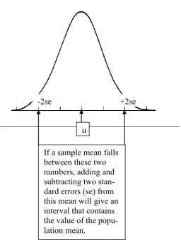
If sample means have a Normal distribution, then the same rule applies to this dis-tribution as any other Normal disdis-tribution. Approximately 95% of the sample means are then found within two standard errors of the population mean. This in-dicates that most sample means are within a “reasonable” distance of the popula-tion mean. The direct consequence of this knowledge is illustrated in Figure 2.3.2.1.

(28)

[image:28.595.143.400.92.433.2]

28

Figure 2.3.2.1. The relationship between the distribution of sample means and the process of finding a confidence interval to estimate the value of the population mean.

2.4 Misconceptions with probabilistic reasoning

2.4.1 Introduction

According to constructivist theories of learning all students come into any learn-ing environment with their own preconceptions that may or may not be correct. Students combine concepts into a schema – a mental representation of an associ-ated set of perceptions, ideas or actions. If new knowledge is understood, this means that a student has successfully assimilated the new information into an

ap--2se +2se

If a sample mean falls between these two numbers, adding and subtracting two stan-dard errors (se) from this mean will give an interval that contains the value of the popu-lation mean.

(29)

29 propriate schema. If the student has an inappropriate or non-existent schema then assimilating later ideas can become difficult, if not impossible (Krause, Bochner, & Duchesne, 2007).

If students have pre-existing inappropriate or non-existent schemas about prob-ability they will not be able to understand statistical inference. Statistical infer-ence relies on the mathematics of probability from the selection of the sample to the drawing of the final conclusions. The literature shows, however, that a per-son‟s intuitive views of probability are often inappropriate or incomplete. These inappropriate or incomplete views may be difficult to detect because probability questions, using examples such as coin tosses, can be simple to answer. As people get older their intuitive perceptions of statistical phenomena, even though inap-propriate, may get stronger, and formal instruction may not correct these intuitive views (Moore, 1990). Furthermore, it has been found that students may use the formal views inside the classroom, but revert to their own intuitive views, whether correct or not, outside the classroom (Chance, delMas, & Garfield, 2004).

Over the last three decades a body of research has been produced on probabilistic reasoning. This research has identified several errors in intuitive reasoning that are described in the following sections.

2.4.2 The contribution of Tversky and Kahneman

(30)

30 the “representative heuristic,” in which probabilities are evaluated by the degree to which A resembles B. If A is very similar to B, the probability that A originates from B is judged to be high. If A is not similar to B, the probability that A origi-nates from B is judged to be low (Tversky & Kahneman, 1982b). This heuristic manifests itself in several forms. The first of these involves the neglect of base rate frequencies and is illustrated the following example. The participants in Tversky and Kahneman‟s study had to assess the probability that “Steve” was a farmer, salesman, airline pilot or librarian. Steve was described as being meek and tidy with a passion for detail. The participants tended to suggest that Steve was a librarian, as he fitted the stereotype of a librarian. In using this reasoning, how-ever, the participants ignored the base rate frequencies, that is, the number of each occupation in the population.

Using this representative heuristic also led participants not to realise that devia-tions from the expected value generated by a random process are more likely in samples of small size. The participants, therefore, expected that 50% of coin tosses would be heads even with a small number of tosses. This expectation was reinforced by a belief in the “fairness” of the laws of chance. Therefore in a series of coin tosses the independence of each event was ignored so that if a series of Tails had been tossed, a Head was regarded as more likely than a Tail. This latter misconception is known as the “Gambler‟s fallacy” (see also Fischbein &

Schnark, 1997).

(31)

31 data (say a very high result) would be cancelled out by further data (say a very low result) instead of being merely diluted by other data (Tversky & Kahneman, 1982b).

Tversky and Kahneman (1982b) described another judgement heuristic that they referred to as “availability” (p. 11). This led the participants to judge the likeli-hood of an event by the ease with which instances of it could be brought to mind. By this heuristic a class that can easily be retrieved will appear more numerous than a class of equal or higher frequency that cannot be so easily retrieved. There-fore the subjects considered words in the form of „_ _ _ _ ing‟ to be more com-mon than words in the form „_ _ _ _ _ n _‟, even though the first example is a subset of the second (Tversky & Kahneman, 1983). This heuristic also led to the participants assuming correlation between variables when, in fact, this correlation does not exist (Tversky & Kahneman, 1982b, pp. 11-13).

(32)

32 (0.10) and then estimated up to allow for the seven tries but again did not make a large enough adjustment (the final probability is 0.52).

2.4.3 Other misconceptions about probability

Since the work of Tversky and Kahneman other researchers have examined peo-ple‟s understanding of probability. Konold (1989) added another judgement heu-ristic to the list, the “outcome approach.” With this heuheu-ristic it was found that par-ticipants in his study made errors because they had a desire to predict the outcome of a single trial in a probabilistic process, and would judge their predictions as correct or not on this single trial. Lecoutre (1992) added the “equiprobability bias,” where two outcomes of different probabilities are judged to be equally probable even when this is not the case. For example, participants in her study judged that if two dice were rolled then a combination of a „5‟ and a „6‟ was equally likely as two sixes. The participants failed to realise that there were twice as many ways of achieving a „5‟ and a „6‟ rather than two sixes.

Fischbein and Schnark (1997) have described what they call the “time-axis fal-lacy” where they found that people can predict the probability of events in the fu-ture, but do not use later knowledge to predict the probability of events in the past. This fallacy can be illustrated with an example.

You have an urn with two white marbles and two black marbles. You take out a white marble. Without replacing it, you take out a second marble. What is the probability that this second marble is also white?

(33)

33 It was found that in answering the second part of this question the participants correctly realised that the second draw could not influence the first draw, but they failed to realise that knowledge of the second draw could be used to determine the probability of the first draw (Falk, 1986).

If a student has poor intuitive ideas on how probabilistic processes work, it can be expected that this student will have difficulty understanding statistical inference and hypothesis testing, which are based on these probabilistic processes. In addi-tion, Garfield and Ahlgren (1988) have found that these problems are exacerbated if the student has poor basic mathematical skills, especially in the use of propor-tions, fracpropor-tions, decimals and percents.

2.4.4 Misconceptions about conditional probability

Because hypothesis testing involves conditional probabilities it is important that students can interpret conditional statements.

Formally, a conditional probability is presented as

The sample space is therefore restricted to points in an event B; that is, only points in A that are in set B are of interest. For example, if the probability of get-ting a king, given that the requirement that the card is a spade, the formula would read

(34)

34 In this case, the only card of interest is the one card that is both a king and a spade, out of the total number of spades. Cards of other suits are not of interest. Watson and Kelly (2009) found that students in elementary school can use infor-mal conditional reasoning with probabilities, and can understand that sampling without replacement affects the probabilities of outcomes of subsequent selec-tions. Students can also calculate conditional probabilities accurately when the data are in the form of a frequency table. However, when conditional statements are put into social contexts, the students‟ background knowledge may interfere with the calculations of these probabilities. The “time-axis fallacy” may also play a part; that is, students can predict the probability of events in the future given past events, but cannot give the probability of events in the past given later knowledge (Fischbein & Schnarch, 1997).

2.5 Other misconceptions about statistical reasoning

2.5.1 Misconceptions about randomness

(35)

35 The varying meanings that students apply to the term randomness have been in-vestigated by LeCoutre, Rovira, LeCoutre and Poiteviniau (2006). Some partici-pants in their study believed that randomness applied for any occurrence where the cause is unknown. If a cause is found, these participants then believed that the occurrence was no longer random. The authors also found that some participants believed that randomness applied to any situation where the probability was easy to compute. Of interest was the finding that a background in probability study had little effect on the accuracy of the participants‟ beliefs. This illustrates how stu-dents‟ intuitive knowledge, while inappropriate, may be difficult to correct (Krause et al., 2007).

2.5.2 Misconceptions about sampling

(36)

36

2.5.3 Misconceptions about measures of central tendency

For students to perform hypothesis tests successfully, they need to understand concepts related to the mean and other measures of central tendency. In particular, it needs to be understood that the arithmetic mean is in some way representative of a group. It is because of this representativeness that many common hypothesis tests are about the mean of a population, or the difference in means of two popu-lations. The calculation of the arithmetic mean, the mode and median are simple, yet students from primary school to the tertiary level have been found to have dif-ficulties with using and understanding these statistics.

(37)

37 above the mean to the mean is equal to the sum of the distances of the data points below the mean to the mean (p. 36).

Once students see the mean as a representative number for a data set, they should also be able to see that this representativeness allows for comparisons of data sets. This understanding should later be extended to making inferences involved in comparing populations (Gal, Rothschild, & Wagner, 1990).

Watson and Moritz (1999) gave students from Grades 6 to 9 a problem that re-quired them to compare two data sets that were presented in the form of graphs. Many of the students did not use the mean in their conclusions, and of those who did (10% of the Grade 6 students and 54% of Grade 9 students), did not always do so successfully. Similarly, for students in Grades 3 to 9, Gal, et al. (1990) found that some students did not use the mean in their comparisons even though they had demonstrated familiarity with the algorithm. In a study of students from Grades 5 to 8, Hancock, Kaput and Goldsmith (1992) also found that some stu-dents did not use means to make comparisons between groups of unequal size, many using totals instead. Hancock et al. (1992) also found that students tended to give individual cases in a group more importance than is desirable. In addition, they would produce graphs if required for their assessments, but then would ig-nore them when drawing their conclusions, indicating that they did not see the representative nature of these forms of data representation either.

(38)

38 of central tendency is most appropriate for a given data set. However, many still have difficulty with these ideas. Pollatsek, Lima and Well (1981) found that when given a situation in which a weighted mean was required, a “surprisingly large proportion” of college students could not calculate it, did not understand the con-cept, and did not recognise that the ordinary mean was not appropriate. Many of these students did not comprehend that an error had been made, even when given follow up questions that were designed to prompt them to recognise their errors. Groth and Bergner (2006) examined the understanding of Grade 12 students and preservice teachers related to the mean, median and mode. They found that most students chose to use the mean of data when it was more appropriate to use the median. Only 7% of these students could discuss which measure was most suit-able for each example they were given. Although some students could explain that the mean and median measured the centre of the data or were in some way representative of the data, there were still students who could only explain these measures in terms of the algorithms used to calculate them.

2.5.4 Misconceptions about statistical inference

(39)

39

2.5.4.1 Misconceptions about variability

Because variation is omnipresent, Reid and Reading (2005) suggested that the success of students in statistics depends on how well they can develop an under-standing of variation in different contexts. The ability to look at a data set, with its variation, as a whole comes with experience. Garfield, delMas and Chance (2007) found that at the beginning of an introductory university statistics course their students tended to focus on individual points, and the range, but not to focus on where most of the data were. They found that extensive practice was needed for students to see the data as a whole. In a study of pre-service teachers, Leavy (2006) found that these teachers concentrated on the summary statistics and ig-nored the variation, rather than focussing on the data as a whole.

Liu and Thompson (2005) studied in detail tertiary students‟ understanding of the standard deviation. The students were required to arrange the bars in a histogram of discrete data so that the highest standard deviation would be produced. Initially the students spread the bars evenly across the x-axis, illustrating they were not considering the standard deviation in terms of total deviation from the mean. Liu and Thompson concluded that few students had a conception of the standard de-viation that combined both frequency and dede-viation from the mean.

2.5.4.2 Misconceptions about sampling distributions and the Central Limit Theorem

(40)

40 conceptual understanding of how statistical inference takes place. DelMas, Gar-field, Ooms, and Chance (2007) found that indeed there are students who cannot use these concepts simultaneously. In particular, they cannot deal with concurrent use of the mean of the sample, the mean of the population and the mean of the sampling distribution.

It has also been found that students may expect sets of data to be normally dis-tributed when this is not the case. Bower (2003) described how some students have a tendency to believe that the larger the sample size, the closer the distribu-tion of any statistic will approximate a Normal distribudistribu-tion, even when there is an obvious lower bound such as zero. These students will believe, therefore, that something is wrong if a non-Normal distribution is found. DelMas et al. (2007) discovered that there are some students who, at the end of a tertiary statistics unit, showed a more fundamental lack in understanding, in that they could not draw a Normal distribution when given its parameters.

(41)

41 consequence, they do not understand that variability among samples means is less than that of the individuals of the population, and that variability among sample means will decrease with an increase in sample size.

Lipson (2002) studied students‟ understanding of the sampling distribution of a statistic (for example, that sample means form a Normal distribution) in contrast to the distribution of the sample (the pattern formed by the individuals in the sample). In her study, 43% of the participants could state that the sample statistic was determined from the sample, and that the variability of this sample statistic is described by the sampling distribution. Twenty two percent of the participants, however, stated that the distribution of the sample (the individuals) was the same as the distribution of the sampling statistic. This left 35% percent of the students who did not clearly indicate their reasoning. Further evidence of difficulties with the distribution of samples was supplied in a study of teachers by Liu and Thomp-son (2005) who found that the participants did not incorporate the idea of the dis-tribution of sample statistics at all, and therefore did not consider whether or not a statistic was unexpected when deciding on the outcome of inferential reasoning. Lipson (2002, p. 1) concluded that the concept of the sampling distribution is “multifaceted and complex” and as a result students find this difficult.

(42)

42

2.5.4.3 Misconceptions about null and alternative hypotheses and their in-terpretation

Part of the procedure for hypothesis testing is to propose a hypothesis about the population of interest. This hypothesis should be falsifiable (see Section 2.3.1) and has to be stated correctly, so that when the hypothesis test is completed an incorrect statement will not be accepted or rejected. Unfortunately, some students do not even realise that the null hypothesis refers to a population, but instead think that a null hypothesis can refer to both a population and a sample (Sotos, Vanhoof, Van den Noortgate, & Onghena, 2007).

A further problem is that the steps can be carried out correctly but the meaning of the results can be misinterpreted as students may have an inappropriate under-standing of what accepting or rejecting a null hypothesis really means. This latter problem was investigated by Haller and Krauss (2002). Of particular interest is that many of their subjects were instructors in undergraduate statistics courses. The researchers surveyed 113 staff and students (including statistics instructors) from psychology departments at six universities. The participants were given the example of an independent samples t-test to determine if there was a significant difference in the means of control and experimental groups. In their example the

P-value was .01. The participants were asked to agree or disagree with each of the following statements.

1. You have absolutely disproved the null hypothesis (that is, there is no dif-ference between the population means).

2. You have found the probability of the null hypothesis being true.

(43)

43 4. You can deduce the probability of the experimental hypothesis being true. 5. You know, if you decide to reject the hypothesis, the probability that you

are making the wrong decision.

6. You have a reliable experimental finding in the sense that if, hypotheti-cally, the experiment were repeated a great number of times, you would obtain a significant result on 99% of occasions.

Eighty percent of the participants who were statistics instructors marked at least of one of these statements as true, while all the psychology students marked at least one of these statements as true. When analysed by statement, Statement 5 had the highest percentage incorrect (average 74%). For this statement it appears that the caveat, “if Ho is true”, was not known, forgotten or ignored. Statements 4

and 6 were the next highest in percentage incorrect (average 47%); while State-ments 1 to 3 were the most often correct (average incorrect 18%).

Further investigation by Haller and Krauss (2002) showed that for some of these students and instructors the results of a hypothesis test was regarded in the same light as a mathematical proof. Thompson et al. (2007) also found in their research this tendency to believe that the results of a hypothesis test indicate proof. Sub-jects, believed that to reject a hypothesis test means that the hypothesis has been proved wrong, and that further evidence in unnecessary.

(44)

44

2.5.4.4 Misconceptions about the interpretation of the P-value and the

level of significance (α)

In the hypothesis testing procedure, the level of significance (denoted by α) indi-cates the level of probability at which the null hypothesis will go from being ac-cepted to rejected. It also indicates the maximum chance of rejecting the null hy-pothesis if this hyhy-pothesis is actually true. The P-value is the probability that given a particular hypothesis about a population parameter, the sample statistic or one even more unlikely, is observed.

Several studies have found a combination of the following misconceptions about the level of significance to be held by both students and researchers. The level of significance may be regarded as the probability that one of the hypotheses is true. The level of significance may also be regarded as the probability of being wrong, or just as the probability of making a mistake (Batanero, 2008; Nickerson, 2000). Similar misconceptions apply to the meaning of the P-value. The P-value is be-lieved by some to be the probability that the null hypothesis is true. The P-value is also interpreted as the probability that the event of interest could happen, given that the null hypothesis is true (Gliner, Leech, & Morgan, 2002). Students may also believe that any one P-value will be replicated if the experiment is replicated. They do not realise that a particular sample statistic is unlikely to be replicated, and, furthermore, do not realise that the probability of having a sample statistic that exactly replicates the null hypothesis is extremely small (Cumming, 2006; Mittag & Thompson, 2000; Nickerson, 2000).

(45)

45 significance also implies practical significance (Gliner et al., 2002). A study of researchers, however, found that these subjects were generally aware that this was not the case (Mittag & Thompson, 2000).

2.5.4.5 General misconceptions about hypothesis tests

Students may carry out hypothesis tests with correct procedures and conclusions, but then give these conclusions unwarranted meanings. For example, if a null hy-pothesis is rejected, students may conclude that the theory behind the experiment is true. If the null hypothesis is accepted, then the experiment might be regarded as a failure (Nickerson, 2000).

Another problem is that students may carry out a hypothesis test, and then look for non-statistical reasons for their conclusions. For example, Lipson, Kokonis, and Francis (2003) found that even when the students in their study verbalised that the likelihood of the sample coming from the hypothesised population was small, they tended to look for a practical explanation (deliberate tampering with the sample, for example) rather than dealing with the statistical solution. Kaplan (2009) found that students rated the results of statistical inference on the strength of their own beliefs. Therefore if they did not believe a conclusion, the students would look at problems in design and ask for further information. They did not do this, however, if they believed the results. The students did not realise that it was necessary to discuss the strengths and weaknesses of any experiment, and not just when they were surprised by the result.

2.5.4.6 Misconceptions about the interpretation of confidence intervals

(46)

popula-46 tion parameter from the sample, with an indication of the uncertainty due to chance variation (Moore, 1990). If, for example, it is stated that the 95% confi-dence interval for the mean is between 20 cm and 25 cm, the value of the popula-tion mean is believed to be between these two numbers (including the end points). To the educated reader, the 95% indicates that the process used will give a correct estimation 95% of the time, but that for any one interval it is not known whether the answer given is correct. That is, the accuracy of the individual result is un-known, but the overall level of uncertainty is known.

In a study of undergraduate students, delMas et al. (2007) found that about one third of students believed that a confidence level indicated the percentage of population values that lie between the confidence limits. These students also had a tendency to believe that the confidence level represents the percentage of sample values within the confidence limits. In addition, the majority of the subjects in delMas et al.‟s study indicated that the level of confidence denoted the percentage of all sample means that lie between the confidence limits. These students did not understand that their knowledge of Normal distributions led to a process that al-lows estimation of the population mean. As a result, they were not able to take the step from the knowledge that 95% of all sample means are within two standard errors of the population mean, to knowledge that this leads to a process that en-ables inference about the population mean.

(47)

47 means that would fall within the original confidence interval if replicate samples were taken.

2.6 The persistence of preconceived views

Students can hold multiple and contradictory views on probability as well as on other topics in mathematics, and on many other physical phenomena (Konold, 1995). In the classroom, students may use the formal methods, but resort to their own intuitive knowledge and methods outside the classroom. Because intuitive beliefs appear self evident and obvious, students are reluctant to change them (Fischbein & Schnarch, 1997). When presented with information that conflicts with their previous views, students may rather look for and find evidence for their misconceptions than use a new theory (Dunbar, Fugelsang, & Stein, 2004;

Shaughnessy, 1992). If the new theories do not fit into the structure provided by their intuitive theories, these new theories are then integrated into their schema with difficulty (Dunbar et al., 2004). It is for this reason that instruction may not correct previously held misconceptions.

2.6.2 How students change their previous conceptions

(48)

48 new paradigm may result that replaces the old paradigm. This will happen, how-ever, only if attempts at articulation fail. Kuhn states: “Only when these attempts at articulation fail do scientists encounter the third type of phenomena, the recog-nised anomalies whose characteristic feature is their stubborn refusal to be assimi-lated to existing paradigms” (p. 97). Strike and Posner (1985) made a similar claim for individuals. Students will not make a major change in a former concep-tion, or form a new concepconcep-tion, until they have found that less radical changes will not work. This change will not take place, however, unless the new/adjusted conception is at least minimally understood, appears initially plausible and has explanatory power. These ideas are further developed in the discussion on theo-ries of learning in Chapter 3.

2.7 Implications of the literature for teaching statistics

For those who teach applied statistics courses, the message from the literature is twofold. Firstly, because it appears that students can successfully complete statis-tics courses using procedural knowledge only, if conceptual understanding is con-sidered to be important, then conceptual understanding will need to be assessed (Kelly, Sloane, & Whittaker, 1997).

(49)

(50)

50

3. Literature Review part II: The nature of learning

3.1 Introduction - What is learning?

If someone says they have “learnt” something, what do they mean? For some people learning has taken place if they can reproduce a series of facts, whereas for others, learning means something more comprehensive. For example, on giving students a text to study, Martin and Säljö (1976) found that some students aimed just to reproduce the contents of the text (“surface learning”), whereas other stu-dents tried to understand the intention of the author of the text (“deep learning”). In a more general context, deep learning, in contrast to learning that merely re-produces content, can be considered to have occurred when the student can under-stand the material, relate parts to a whole, integrate it with existing knowledge and apply it in real world situations (Boulton-Lewis, 1995).

(51)

51 the process of abstraction and theory building (Krause et al., 2007; Mason & Spence, 1999).

With this in mind it can be said that students who can complete their statistics courses but cannot explain the reasoning behind what they do have achieved sur-face learning or procedural knowledge, and have not achieved theoretical knowl-edge or deep learning.

3.2 How learning occurs

One aim of this research was to discover students‟ understanding about probabil-ity and hypothesis testing so that the teaching of statistics to first year universprobabil-ity students could be adapted to make deep learning more likely to be achieved. From reading students‟ work in the past it was clear that some of these students had ideas about statistical inference and hypothesis testing that were not in their lec-ture notes, not in their text, and were never presented to them in their leclec-tures or tutorials. These students were not merely reproducing what they had learnt or read, but were somehow processing this information for themselves.

(52)

52

3.2.2 Information processing theory

Information processing theory states that human memory does not simply retain information but is an active system. This system actively selects the sensory data that are to be processed, transforms the data into meaningful information, and stores much of the information for later use. Learning comes about when informa-tion from the environment is transformed into cognitive structures.

Several models have been proposed to describe how human memory works. The first to be described here is the “multistore” model (Krause et al., 2007). Accord-ing to this model, information is noted by the senses and if attention is paid to the information, it will be transferred to the short term memory. If the information is considered important enough it will be transferred to the long term memory, if not, it will be forgotten. This long term memory is made up of episodic memory, which holds memories of personal events, semantic memory, which holds lan-guage and knowledge of how the world works, and procedural memory, which holds knowledge of procedures for performing the skills we need (Krause et al., 2007).

An alternative model is called the “levels of processing model” where attention is paid to the level of information processing. According to this model “deep proc-essing” occurs when information is analysed and enriched by making connections with existing knowledge. Information that is analysed more deeply will be re-membered (Krause et al., 2007).

(53)

in-53 tended by the lesson. They also can help instructors to understand why students may not retain information they have been given. Learners may not retain infor-mation because they have failed to pay adequate attention, they may be not moti-vated to remember, they might have inadequate memory skills, or they might not have the right cue to recall the information. These problems may be exacerbated if students are taught in a didactic way (Perkins & Simmons, 1988). Learners may also not retain the information because the short term memory is limited (Krause et al., 2007). Consequently, if too much new information is given at once, stu-dents will not be able to process this information effectively (Wieman & Perkins, 2005).

3.2.3 Constructivist theories of learning

Constructivist theories, like information processing theories, suggest that learners are not passive recipients of knowledge, but play an active part in their own learn-ing. Rather than learners passively receiving knowledge as it is given, learners actively construct new knowledge by linking it to prior knowledge and under-standing. It is argued by some (radical constructivists) that knowledge, no matter how it be defined, is in the heads of persons, and that as a result learners have no alternative but to construct what they know on the basis of their experience (von Glaserfield, 1995).

(54)

54 particular meanings are given to the events and objects that are encountered, and therefore all learning is socially mediated (Tobin, Tippins, & Gallard, 1994). According to constructivism, learners operate with a schema. A schema is a clus-ter of ideas about a particular object or experience that is used by the person to organise existing knowledge in a way that makes sense. When learners come across a new situation, they may be able to assimilate the new knowledge into a pre-existing schema without modification. If an inconsistency arises between new information and a current schema, learners experience disequilibrium, and then have to modify the existing schema by the process of accommodation (Krause et al., 2007).

Using constructivist theory, Perkins and Simmons (1988) described how errors may occur as students acquire new information.

 Students may have naïve, underdifferentiated, and malprioritised concepts that may rival and override those of the new topic.

 Students may have difficulty accessing freshly acquired knowledge, espe-cially if it was given in a didactic fashion.

 Students may mix up the new knowledge in various ways, and the result is a garbled version of what was intended.

 Observations that do not fit into their previous intuitions may be ignored, and only observations that fit into these prior intuitions will be acknowl-edged (see Section 2.6.1).

(55)

55 If Perkins and Simmons are correct, then students will resist the process of ac-commodation; that is, they will prefer to hold to a view of the world that is inter-nally inconsistent rather than go through the process of modifying an existing schema. Students will only modify an existing schema if something easier will not work, and if the new schema is in some way plausible.

3.2.4 Implications of the cognitive models for teaching

If we accept that learners construct knowledge and understandings based on what they already know and believe, then it would seem important that instructors should discover what knowledge their students have, and what their problems are likely to be. “It is easier to orient students towards a particular area of conceptual construction if one has some idea of the conceptual structures they are using at present” (von Glaserfield, 1995, p. 185).

If students have prior conceptions that are not consistent with what is being taught, instead of undergoing the process of accommodation, they may build fur-ther misconceptions, or use what is being taught inside the learning environment but use their own ideas outside it (Bransford, Brown, & Cocking, 2000). Because these students are using what is taught inside the learning environment they may appear to have made an accommodation when, in fact, they have not done so. Strike and Posner (1985) stated:

(56)

56 The cognitive models of learning therefore suggest that instructors, being aware of likely problems, should give their students opportunities to work through new material and should give them the time needed to come to terms with it. These models also suggest that the instructors need to monitor their students‟ under-standing to check that an appropriate assimilation or accommodation has taken place.

Information processing models suggest that instruction should be designed to as-sist students to store new information in the memory by attracting the learners‟ attention to the relevant information and organising this information in a way that makes it easy to assimilate (Krause et al., 2007). They also suggest that only a certain amount of new material should be given at one time.

3.3 Affective factors

It would be expected that instructors who are keen for their students to gain con-ceptual understanding, and, it must be said, achieve good grades, will usually try to develop the best program possible for their students. However, the aims of the instructors may be thwarted by the beliefs and aims of their students, which may not coincide with theirs. Pintrich, Marx and Boyle (1993) stated:

The assumption that students approach their classroom learning with a rational goal of making sense of the information and coor-dinating it with their prior conceptions may not be accurate. Stu-dents may have many social goals in the classroom context be-sides learning – such as making friends, finding a boyfriend or girlfriend, or impressing their peers – which can short circuit any in-depth intellectual engagement. (p. 173)

(57)

57 Even if the focus is on academic achievement, students may adopt

different goals for or orientations to their learning. For example, it appears that a focus on mastery or learning goals can result in deeper cognitive processing on academic tasks than a focus on the self (ego-involved) or a focus on performance (grades, besting others), which seems to result in more surface processing and less overall cognitive engagement (Pintrich et al., 1993, p. 173).

(58)

58

3.4 The use of the SOLO taxonomy in assessing learning

Piaget suggested that as people grow older they have increasingly more complex ways of reasoning available to them (Krause et al., 2007). At first children learn using concrete modes, and as they grow older they are able to use increasingly abstract modes of reasoning. Biggs and Collis (1982) suggested that there are natural stages in the growth of learning of any complex material that are analo-gous to the developmental stages of reasoning described by Piaget. As a result Biggs and Collis developed a system for assessing learning (The SOLO Taxon-omy – Structure of Observed Learning Outcomes) that takes into account the demonstration of increasingly abstract knowledge and increasing complexity of the learner‟s reasoning. In this system, an answer that does not address the ele-ments of a task is considered to be “Prestructural.” An answer that employs a sin-gle element of the task only is considered to be “Unistructural,” whereas an an-swer that employs several elements in a task is considered to be “Multistructural.” Those answers that create connections among the elements of a task to form an integrated whole are considered to be “Relational” (Watson & Callingham, 2003). Using the principles of the SOLO model, a form of assessment can be developed where students are not only assessed on right/wrong answers, but can be assessed on the level of sophistication of their reasoning.

(59)

59 of a coin coming up with a Head after four Tails had come up in a row, and to give an explanation for their answer. Those students who did not address the task were considered to give a Prestructural response and received a code of “0.” Those students who answered that as there were “only two outcomes” the prob-ability is 0.5 were considered to give a Unistructural response and received a code of “1.” Those students who added that as the toss of coin is “not affected by the outcomes of previous tosses” the probability is 0.5 were considered to give a Multistructural response, as this response indicates that the students were consid-ering more aspects of the overall picture. These students received a code of “2.” If a student had considered the pros and cons of the competing explanations would have been considered to give a Relational response (no student did this).

(60)

60

4. Literature review part III: Measurement in the

so-cial sciences

4.1 Scales used in measurement

Measurement can be defined as the assignment of numbers to objects or events according to rules (Stevens, 1946). The attributes of the things being measured determine the scale that applies the numbers, and in turn the scale determines the mathematical properties of the measurements and the statistical operations that can be applied to the measurements.

The simplest form of measurement uses a nominal scale where numerals are used only as labels. For example, a “1” may be used for a person enrolled in a Bachelor of Arts, and a “2” may be used for a Bachelor of Science. With a nominal scale numerals are used only as labels and no order is implied with these numerals. In general, the only statistic available for nominal data is the number of cases in each category. Yet even though nominal data have no implied order, nominal data such as race or gender may still be important explanatory variables (Wright & Linacre, 1989).

(61)

dis-61 tances each step may require (Wright & Linacre, 1989). For example, it might be harder to go from “average” to “extensive” than from “none” to “average”. The next level of complexity involves the use of an interval scale where the inter-vals are equal (Stevens, 1946). Such scales are often used in the physical world and are often simple to understand. For example to measure length a particular item of interest is matched against another length that has been standardised in some way, for example, marked in centimetres. The measurement of length also involves a “ratio” scale. By this it is meant that a zero length is a true zero, as it is not possible to have a length that is less than zero, and 20 cm, for example, is twice as long as 10 cm.

The measurement of temperature also involves an interval scale but the process of measurement is indirect. In a common mercury thermometer temperature (in Cel-sius or Fahrenheit) is measured by the expansion of mercury in a calibrated glass tube, unlike the measurement of length where a length is lined up against a stan-dard length. There is another important difference between these measuring scales. Whereas temperature measured on the Celsius or Fahrenheit scales uses interval scales these are not ratio scales. This is because it is possible to have a temperature below zero, and 20o_{, for example, is not twice as hot as 10}o_{on either}

scale.