Embedded control system for biogas digesters

(1)

University of Southern Queensland

Faculty of Engineering & Surveying

Embedded Control System for Biogas Digesters

A dissertation submitted by

T. Sullavan

in fulfilment of the requirements of

ENG4112 Research Project

towards the degree of

Bachelor of Engineering, Mechatronics

(2)

Abstract

Biogas is also known as dump gas, marsh gas or sewer gas and is produced in a

com-mon, naturally occurring biological decomposition process. It is composed mainly of

methane, CH4, carbon dioxide, CO2, and hydrogen sulphide, H2S. Smaller quantities

of hydrogen, H oxygen O2, nitrogen, N and ammonia, NH3 may also be present.

Methanogens occur naturally in the digestive systems of ruminant animals such as

cattle, in marshes, brackish waters and sewage works, where, in addition to laboratories,

much knowledge of them has been gained.

Literature review reveals that biogas production and thus rate of decomposition is

influenced by temperature, and additionally that the loading conditions of a digester

may be deduced by monitoring the concentrations of individual component gasses of

the biogas produced.

It is the objective of this project to:

• Develop an electronic nose to monitor the biogas composition,

• Develop a fuzzy logic controller to increase or decrease the temperature of the

digester vessel, thus controlling the rate of decomposition, and

(3)

University of Southern Queensland

Faculty of Engineering and Surveying

ENG4111/2 Research Project

Limitations of Use

The Council of the University of Southern Queensland, its Faculty of Engineering and

Surveying, and the staff of the University of Southern Queensland, do not accept any

responsibility for the truth, accuracy or completeness of material contained within or

associated with this dissertation.

Persons using all or any part of this material do so at their own risk, and not at the

risk of the Council of the University of Southern Queensland, its Faculty of Engineering

and Surveying or the staff of the University of Southern Queensland.

This dissertation reports an educational exercise and has no purpose or validity beyond

this exercise. The sole purpose of the course pair entitled “Research Project” is to

contribute to the overall education within the student’s chosen degree program. This

document, the associated hardware, software, drawings, and other material set out in

the associated appendices should not be used for any other purpose: if they are so used,

it is entirely at the risk of the user.

Prof F Bullen

Dean

(4)

Certification of Dissertation

I certify that the ideas, designs and experimental work, results, analyses and conclusions

set out in this dissertation are entirely my own effort, except where otherwise indicated

and acknowledged.

I further certify that the work is original and has not been previously submitted for

assessment in any other course or institution, except where specifically stated.

T. Sullavan

0050011624

Signature

(5)

Acknowledgments

Special thanks go to the supervisors of this project, Dr Selvan Pather and Mr Mark

Phythian for their invaluable guidance, and to my family and fiance for their unending

patience and tolerance throughout the duration of this project and my studies. I could

have achieved little without them.

T. Sullavan

University of Southern Queensland

(6)

List of Figures

1.1 Biogas Control System Proposal . . . 3

2.1 Types of continuous flow digesters. (Fry 1973). . . 6

2.2 Digester indicators, conditions, and remedies. (Stafford, Hawkes & Horton 1981). 9 2.3 Methane and hydrogen levels - no control. (Murnleitner, Becker & Delgado 2002). 10 2.4 Methane and hydrogen levels - with control. (Murnleitner et al. 2002). 10 3.1 Photo of main board with Atmega 8 microcontroller and peripherals. . . 14

3.2 Main board with microcontroller, serial line driver and voltage regulators. 16 3.3 E-nose with op-amp, and temperature and gas sensors in chamber. . . . 17

3.4 Thermistor connections to LMC660CN op-amp. . . 18

3.5 MG811 CO2 sensor connections to LMC660CN op-amp. . . 20

3.6 TGS2611 CH4 sensor connections to LMC660CN op-amp. . . 21

3.7 MQ7 H2 sensor connections to LMC660CN op-amp. . . 22

(11)

LIST OF FIGURES x

4.1 Main function flowchart. . . 26

4.2 Controller initial input membership functions used to fuzzify. . . 29

4.3 Controller response to an input of -20. . . 31

4.4 Controller response to an input of -10. . . 31

4.5 Controller response to an input of 0. . . 32

4.6 Controller response to an input of +5. . . 32

4.7 Controller response to an input of +20. . . 33

4.8 Temperature set point for expected d(CO2)/dt levels. . . 34

4.9 Modified Temperature set point for expected d(CO2)/dt levels. . . 35

4.10 Modified temperature set point for expected d(CO2)/dt levels. . . 36

4.11 Captured temperature set point for expected d(CO2)/dt levels. . . 37

4.12 Captured modified temperature set point for expected d(CO2)/dt levels. 37 5.1 Dilution equipment used throughout laboratory tests. . . 40

5.2 Captured data from CO2 sensor; trial 1. . . 43

5.3 Captured data from CH4 sensor; trial 1. . . 43

5.4 Captured data from H2 sensor; trial 1. . . 44

5.5 Captured data from CO2 sensor; trial 2. . . 44

(12)

LIST OF FIGURES xi

6.1 Trial 3 CO2 concentrations using logarithms. . . 50

6.2 Trial 3 CH4 concentrations using logarithms. . . 50

6.3 Trial 3 H2 concentrations using logarithms. . . 51

6.4 Resulting temperature setpoint using captured data. . . 53

6.5 Gas inputs against temperature setpoint; case 1. . . 55

(13)

Chapter 1

Introduction

1.1

Background

1.1.1 History

The methanogenic bacteria appear to be ancient forms of life. Hydrogen and oxygen

outgassed from the Earth’s mantle could well have supported the existence of these

organisms long before the development of primitive plant species hundreds of millions

of years ago. Anaerobic digestion of biomass has occurred throughout the existence

of life on Earth, and is therefore expected to be a highly reliable, stable and efficient

process in those environments where it occurrence is essential to maintain the natural

cycle of organic matter (Smith, Bordeux, Goto, Shiralipour, Wilkie, Andrews, Ide &

Barnett 1988).

The identification of a specific gas from the anaerobic digestive process was first made

by Volta in 1776. ‘Inflammable air’ was found to be readily generated (Stafford

et al. 1981). It has been used for at least a century in developing countries for the

decomposition of animal and human waste, in most cases from a necessity to maximise

the benefit from limited available resources in rural areas. While the combustion of cow

dung for cooking provided a renewable source combustible fuel, it was at the expense of

(14)

1.1 Background 2

rural kitchen. Exposed human waste encourages vermin and diseases. In response,

anaerobic digesters were developed to decompose the waste to provide a rich organic

fertiliser for crops and a fuel gas to power household lighting and stoves.

1.1.2 Ethics

As it stands at the moment, the time has come to address serious shortcomings in our

current socio-economic direction. Numerous mineral fuel supply interruptions, price

spikes, bloody international conflicts, and more recently, revelations concerning global

warming and environmental degradation have stimulated interest in current energy

sources. The human race is facing increasing problems associated with disposing of

waste produced directly by the population, and by the agricultural and industrialised

systems we use to feed and otherwise occupy ourselves. Soils used by mass commercial

crop cultivation methods are also increasingly showing signs of degradation due to

intensive farming paractices reliant on the extended use of chemical fertilisers and

pesticides, often also based on mineral oil derivatives.

Reflection on the benefits and surrounding issues has led to belief that the utilisation

of anaerobic digestion to produce biogas could play an important and profitable role in

addressing a wide variety of social and environmental issues faced by human beings as

we enter the 21st century. The production of human and animal waste is independent

of crude oil supplies and available to a much wider demography. Biogas combustion

produces only a fraction of the pollution of fuels and energy systems widely used today,

and competition for the raw materials required for biogas production are unlikely to

cause conflict. The effluent of anaerobic digesters can be used to organically nourish

and restore fertility to agricultural soils and hydroponics, without the health concerns

associated with chemicals. While techniques to achieve anaerobic decomposition have

been ongoing areas for research across the world for some time, many installations

could benefit from modern technology and safety features, resulting in improved

bio-gas yields, improvements in plant safety, and reduced and better targeted operational

(15)

1.2 Objectives 3

1.2

Objectives

The objective of this project is to improve the safety and performance of small digester

systems by:

1. Developing and constructing an array of gas sensors otherwise known as an e-nose

to monitor biogas composition,

2. Developing an embedded controller to monitor and control a digester vessel,

3. Adding user interface to notify personnel of the state of the digester.

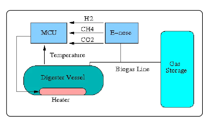
[image:15.595.137.489.368.572.2]

1.3

Methodology

Figure 1.1: Biogas Control System Proposal

1. The monitoring of hydrogen H2, carbon dioxide CO2, and methane CH4 in the

gas economically and effectively in order to provide sufficient data to allow reliable

data concerning the health of the digester.

2. The development of an embedded micro-controller hardware and software using

fuzzy logic to control the system by autonomously maintaining appropriate

(16)

1.3 Methodology 4

3. The microcontroller is to notify personnel of the requirements of the system

through a system of semaphore lights. This information should indicate digester

health/ overload conditions as appropriate.

A simple digram of this proposal is included in Figure 1.1.

To achieve this, the following course of action should lead to the achievement of the

objectives: The system hardware must first be developed to permit monitoring of

the target gasses. The sensors may then be connected to the micro-controller. This

will permit testing of the gas sensors in the presence of pure samples of the target

gas samples and derivation of algorithms to process the readings and estimate gas

composition. Software may then be developed interpret the readings and to and set a

(17)

Chapter 2

Biogas

2.1

Chapter Overview

This chapter describes details concerning the composition and production of biogas. It

then goes into aspects of control of a simple biogas digester system.

2.2

Properties of Biogas

Biogas is also known as dump gas, marsh gas or sewer gas and produced in a common,

naturally occurring decomposition process. It is composed mainly of methane CH4,

carbon dioxide CO2, and hydrogen sulfide H2S. Smaller quantities of hydrogen H2

oxygen O2, nitrogen N, and ammonia NH3 may also be present. The component most

responsible for the flammability of biogas is the methane, which usually makes up to

70%of the composition. Carbon dioxide makes up the majority of the remainder with

smaller quantities of hydrogen sulfide, which gives raw biogas its distinctive rotten

egg smell. This can easily be removed by simple scrubbing techniques. Otherwise the

biogas resembles natural gas in composition, with a slightly lower energy content. AS

4564-2005 table 3.1 imposes limits on the composition of general purpose natural gas,

necessitating additional scrubbing of biogas in most cases for compliance if a biogas

(18)

2.3 Biogas Production 6

2.3

Biogas Production

Biogas is a product of anaerobic decomposition by methanogens, a group of bacteria

characterised by their ability to produce methane. These bacteria flourish only in

the absence of oxygen; 0.01mg/L is enough to completely inhibit growth (Stafford

et al. 1981). They occur naturally in the digestive systems of ruminant animals such as

cattle, in marshes, brackish waters and sewage works, where in addition to laboratories,

much knowledge of them has been gained.

Methanogenic decomposition is a complex series of bio-reactions far beyond the scope of

this dissertation, but the basic mechanism relies on the co-ordinated use of two different

heterogenic groups of bacteria. The first are responsible for the decomposition of lipids,

lignins, proteins ands into H2, CH2 and volatile fatty acids (VFA’s). The second type

are the methanogens, which further decompose the products of the first reactions to

form CO2 and CH4.

Digestion is the creation of an artificial environment to encourage Methanogenic

de-composition, about which considerable research has been published.

Figure 2.1: Types of continuous flow digesters. (Fry 1973).

Most digesters in operation are regularly fed with human, animal, or organic

indus-trial waste and produce biogas and an organic sludge, low in pathogens and high in

(19)

feed. Small scale digesters generally make use of a single reaction vessel, and may be

batch fed and sealed until gas production stops, or continually fed, using an internal

system of pipes and gravity to maintain a constant operating level as shown in Fig. 2.1.

Other types of varying degrees of sophistication are used in larger installations. It is

commonly suggested that feed with a carbon to nitrogen ratio, C:N from 20:1 to 30:1

is desirable, and an operating pH of 7 or just over is optimum for the methanogenic

bacteria (Hobson, Bousfield & Summers 1981).

There are two temperature ranges over which anaerobic digestion is most effective. The

mesophillic, usually from ambient to 42 deg C, and thermophillic from 55 to 70 deg

C. In practice, few digesters operate in the thermophillic zone because of the extra

energy required for heating and less stable micro-biological environment. A

tempera-ture around 35 deg C is common to maximise biogas yield whilst minimising digester

retention time and heating energy demands. The microbes are reportedly sensitive

to changes in operating conditions, so once they have acclimatised to the conditions

of a particular digester, sudden fluctuations in temperature or feed material are not

recommended due to the destabilisation of the reactions.

The digestate material must also be agitated to a degree to promote a homogeneous

mixture, prevent micro-biologically dead zones and reduced the build up of scum, which

is a substrate consisting of lighter fractions and fibrous material such as hair and

feathers. The latter can cause significant problems when it hardens on the surface and

prevents the escape of gas from the slurry. Careful design of vessel parameters such

as operating level, gas outlet position, maintenance and slurry agitation can greatly

reduce or eliminate problems with scum.

An additional problem with anaerobic digesters is instability caused by toxic, organic

or hydraulic overload (Stafford et al. 1981). Toxic overload can be caused by

contami-nation of the feed by substances which inhibit the digestion process. Organic overload

is commonly caused by variations in feed consistency or too short a detention time.

Hydraulic overload occurs when the feed material is low in solids and retention time

is reduced to compensate, flushing out the microbial population. For each of these

conditions, there are indicators which may be monitored to allow anticipation of such

(20)

For the purposes of this research project, overload occurs when the methanogens are

unable to keep pace with the first group of bacteria responsible for breaking down

the more complex compounds. These bacteria tend to be more robust and multiply

more rapidly than the methanogens. When this occurs, the methanogens are unable

to consume the VFA’s as they are produced. This has the effect of lowering the pH

of the substrate below that which the methanogens can survive, which is only between

pH 6.4 to 7.5. This results in the poisoning of the methanogens and digester failure.

Stafford et al (Stafford et al. 1981, p77-78) compiled an inexhaustive list of these

conditions and indicators, and suggest possible remedies as included below. These

correspond to the diagram in Figure 2.2.

• Common Faults

A)Toxic Overload

B)Organic Overload

C)Hydraulic Overload

• Typical warning sign

i)methane production falls

ii)The direction of response curves of several variables when compared with

one another can warn of potential failure; for example, VFA rises as the CH4

production falls

iii)The sign of the second derivative of common variables with respect to time

changes; for example:

A concave upward change in the slope of percentage CO2

A concave upward change in the slope of pH

A concave downward change in slope of rate of CH4 production

(21)

2.4 Digester Control 9

1)Solids recycle

2)Increase frequency of loading

3)Adequate mixing

4)Scrubbing gas to remove CO2 before recycle

5)Addition of a base

6)Recycle micro-organisms

7)Reduce or stop feed

8)Increase initial substrate conditions

9)Add plant effluent to feed

Figure 2.2: Digester indicators, conditions, and remedies. (Stafford et al. 1981).

2.4

Digester Control

More recent research has resulted in something of a trend towards the use of fuzzy logic

control systems to monitor and control digester performance. Such systems have

suc-cessfully been implemented in scale laboratory models of wastewater treatment systems

using fluid bed reactor type digesters by Murnleitner et al and Muller et al.

Stafford (Stafford et al. 1981, p78) suggests the monitoring of methane production,

VFA levels, CH4 production, as well as CO2 and pH levels and their second derivatives

with respect to time as a method of monitoring a model fluid bed reactor.

(22)

2.4 Digester Control 10

monitored parameters using off the shelf type sensors. The monitoring methane and

hydrogen levels, pH gas flow and oxidation-reduction potential and conductivity are

included. The results of their research show that hydrogen and methane levels in the

gas accurately reflect the health of the digester. If gas composition data is unavailable,

pH levels are used. They conclude that methane and hydrogen levels, pH and gas flow

are all that are needed to recognise overload conditions.

Figure 2.3: Methane and hydrogen levels - no control. (Murnleitner et al. 2002).

Figure 2.4: Methane and hydrogen levels - with control. (Murnleitner et al. 2002).

Figure 2.3 shows methane and hydrogen levels leading up to an overload. This data was

gathered without control. Notice distinctive increases in hydrogen and corresponding

drop in methane production. This is due to the inability of methanogens to consume

(23)

2.5 Safety Considerations 11

a corresponding, though delayed increase in VFA’s and reduction in pH. Figure 2.4

shows methane and hydrogen levels with the controller. No such indication of overload

is present.

Muller et al (Muller, Marsili-Libelli, Aivasidis, Lloyd, Kroner & Wandrey 1997) adopt

an even simpler approach using a fluid bed reactor; hydrogen level and biogas

pro-duction are used to distinguish between all three overload conditions using this simple

method. Problems with this system could arise if feeding is irregular, such as with a

batch type digester (Murnleitner et al. 2002).

Whilst these two experiments have made great gains in controlling the digestion

pro-cess, the fluid bed reactors in use rely on the co-ordinated use of two vessels with

sludge recirculation and buffering systems. Further advantage is taken of individual

conditions between the stages of the fermentation processes. These systems are able to

greatly stabilise the microbial environment and are fine models for automated,

large-scale wastewater installations. For the objectives of this project, the laboratory

condi-tions are stable and equipment is considered too complex to implement on small scale

community and farm digesters, which are often more simply constructed and operated

under less than optimal conditions.

2.5

Safety Considerations

Whilst most digesters operate at pressures far below the limits set for pressure vessels

in AS 1210-1997, there is a significant risk of excessive pressure in a digester resulting

in the combustion-less explosion of the vessel. This can be due to a number of possible

fault conditions, such as a blocked gas or sludge outlet, or incorrect valve operation.

Therefore, some kind of safety pressure relief arrangement is commonly recommended,

burst disks being about the simplest and most reliable. Being a once-off solution, these

have the disadvantage of replacement in the event of a breach.

Methane is an odourless gas and mixtures of 5-15% methane in air pose a substantial

risk of explosion resulting in serious injury or death. AS 4654-2005 Table 3.1 imposes

(24)

2.6 Chapter Summary 12

the start-up of a new digester or due to leaks, although the internal pressure of the

system usually means a loss of biogas rather than the entrance of oxygen.

Hydrogen sulphide (H2S) is also extremely toxic to humans and 0.002%is the maximum

allowable concentration for prolonged exposure. Higher concentrations of H2S poses a

significant risk of injury or death.

The likelihood of excessive concentrations of CH4, CO2, H2S or any gas in a confined

space is slight, but may result in serious illness or death.

Safety measures such as regular inspection for leaks, effective ventilation and

elimina-tion of ignielimina-tion sources minimise the risks and shall be followed at all times throughout

the duration of this project. It is also desirable to have an additional device to allow

the release of gas and/ or sludge in case of the presence of oxygen, poor quality gas, or

excessive pressure in the vessel, regardless of the cause.

2.6

Chapter Summary

This chapter has outlined relevant details surrounding composition and production of

biogas, and control of a digester. It concludes with safety precautions which must be

adhered to throughout the duration of this project and when dealing with toxic and/

(25)

Chapter 3

Electronic Hardware

3.1

Chapter Overview

Embedded systems are small computer systems tailored to a particular application,

usually powered by a microcontroller suited to the task. In order to gain useful

infor-mation regarding the physical environment in which the embedded system is to operate,

it must be interfaced to a series of sensors designed to provide such information. As

these sensors are the only means for the system to gain this data, the success or failure

of an embedded controller rests heavily on signals it receives from them. Such data

concerning ambient odours or gas concentrations are often determined in electronic

systems by a gas sensor array known as an electronic nose or e-nose.

This chapter contains detailed information regarding micro-controller, temperature and

gas detection sensors, and e-nose circuits.

3.2

Microcontroller

Choice of microcontroller for the project was made by comparison of features,

pro-gramming environment and cost. Accommodating analogue signals from the e-nose

(26)

3.2 Microcontroller 14

Figure 3.1: Photo of main board with Atmega 8 microcontroller and peripherals.

signals from sensors. Demand for memory space was considered to be modest, whilst

large response time constants of most digester vessels places no extraordinary demands

on the processor speed. Required outputs are simple digital ones or zeros to control

the heater, indicator lights and ancillary equipment. Past experience with several

em-bedded system projects has shown that pulse width modulation (PWM) is often useful

if available, while input/ output (I/O) pins are often running scarce towards the later

stages of an experimental embedded system project, and also carried some weight in

the selection process.

Several microcontrollers were considered for the project, the Motorola HC12 family

and Microchip’s PIC series were also considered. The Motorola chips, despite having

many relevant features and specific fuzzy logic instructions, were considered excessive

for this project. The Microchip PICs were also considered, again having many of the

required features, but do not lend themselves to high language programming, and such

well established development environments are not free.

The Atmega 8 microcontroller was chosen due to its availability, cost, features and

(27)

3.3 E-nose 15

MHz oscillator, 8 kbytes of programmable flash memory for programs and data, 512

bytes of EEPROM memory, USART for serial communication, 3 timers and a total

of 23 programmable pins for miscellaneous I/O, 6 of which may be used as ADC’s.

Additionally, 3 pins are configurable for PWM which, although considered unnecessary

initially for this application, was used to provide the two precision voltages for the H2

sensor and may be useful for proportional heating at a later stage.

Available software development environment was also considered. For the Atmega

8, the C programming environment the development tools comprised of the avr-gcc

compiler, avrlibc, avrdude programmer, and avrsim simulator permit a free software

development environment for anyone using a Unix based PC. An MS Windows

envi-ronment is also available. Significant literature, code snippets, makefiles and tutorials

are freely available with the development tools and dedicated webpages.

The circuit diagram in Figures 3.1 and 3.2 shows the embedded controller circuit

di-agram with peripherals. Notice this main circuit board also provides regulated power

supplies to the e-nose through the nine core shielded cable.

3.3

E-nose

E-noses in general have recently received a lot of interest due to their possible

appli-cation to numerous fields such as process control, air quality monitoring, security and

drug detection.

The e-nose construction comprised of three gas sensors for methane, carbon dioxide

and hydrogen and a resistive type temperature sensor, all connected to an LMC660CN

low power quad channel operational amplifier (op-amp). This arrangement requires

regulated voltages to power the amplifier and a total of about 2 watts (W) of power to

heating elements in the gas sensors. It plugs directly into the main circuit board via

nine core shielded cable in order to receive all power and provide analogue signals to

the analogue to digital converters (ADC’s) of the micro-controller.

(28)

[image:28.595.146.490.102.467.2]

3.3 E-nose 16

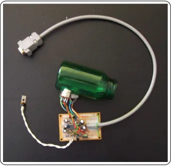
Figure 3.2: Main board with microcontroller, serial line driver and voltage regulators.

a consistant gas composition while samples were taken. To form the sensor chamber,

the three gas sensors were inserted into holes in the side of an empty plastic vitamin

bottle which had been washed with detergent and thoroughly rinsed. Figure 3.3 shows

the completed e-nose assembly.

3.3.1 Amplifier

The LM324 op amp was originally selected for the positioning of individual op-amp

channels within the package, its ability to operate from a single supply rail, and

famil-iarity with the device.

(29)

[image:29.595.148.489.104.436.2]

3.3 E-nose 17

Figure 3.3: E-nose with op-amp, and temperature and gas sensors in chamber.

were connected to the individual strands of 9-core shielded cable via a one kilo ohm

(kΩ) resistor to protect the amplifiers from overloading by limiting the current to

approximately 5 milliamps (mA). This was then grounded via 100 micro fared (µF) capacitors to short AC components from the signal. This can bee seen in each of the

individual sensor circuit diagrams.

Unusually high input impedance demands of the amplifier by the CO2 sensor resulted

in replacement of the LM324 with the LMC660CN op-amp, which is a pin for pin match

with the LM324. The input impedance of over 1 Tera ohm (TΩ) and input bias and

(30)

3.3 E-nose 18

3.3.2 Sensors

Gas sensors were selected on the basis of individual gas sensitivity, cost and availability.

Three sensors were selected:

• The CO2 sensor was the MG811 by Hanwei Electronics.

• The MQ7 for H2, also by Hanwei.

• The TGS2611 by Figaro for CH4.

Manufacturer’s datasheets indicate that all of these sensors return either linear or

logarithmic inputs for logarithmic variations in gas concentrations. Ambiguous data

sheets meant considerable trial and error to obtain acceptable results.

The temperature sensor was a simple linear resistive sensor with a resistance of 50 kΩ

at room temperature. This was placed in series with two other resistors and the voltage

measure by a differential feedback amplifier. The circuit diagram is shown in Figure

[image:30.595.144.490.462.668.2]

3.4.

Figure 3.4: Thermistor connections to LMC660CN op-amp.

Of concern to this project is expected cross-sensitivity of the TGS2611 CH4 sensor

to H2. It is proposed that this be resolved by choosing a hydrogen sensor which is

(31)

3.3 E-nose 19

scalar multiple of the H2 reading from the methane reading. Both Figaro and Hanwei’s

datasheets include information regarding sensitivities to other gases.

Of additional concern is the concentrations at which these sensors can provide valid

readings; composition of biogas is measured as percentages, while these sensors are

generally operated in concentrations of under 10 000 parts per million (ppm) in air.

The simplest method to achieve this is to precisely dilute sampled biogas with air in

order to carry out reliable analysis. This is covered in Chapter 5.

3.3.2.1 MG811 Carbon Dioxide Sensor

As CO2 sensors are the most easily obtained, much development of the e-nose and

software was based on trials with these. Great confusion was caused by ambiguity of

the datasheet, particularly conflicting output voltages and input impedance required of

the signal amplifier. The literature specifies such amplifiers have an input impedance

of 100 to 1000 GΩ, which resulted in the premature failure of two of these sensors and

hours of troubleshooting.

The CO2 sensor requires a precision 6 volt (V) supply and 200 mA for the heater. This

was provided by a 3 terminal regulator on the main controller board. It is an EMF type

sensor, thus producing a voltage inversely proportional to CO2 concentration. Hanwei

states that the maximum sensor output is 300 mV at atmospheric concentrations of

CO2. It is designed to return a linear EMF to logarithmic gas concentrations from 350

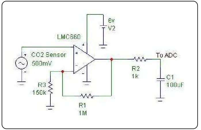
to 10 000 ppm. The CO2 sensor datasheet gives no indication of sensitivity to H2.

The op-amp was placed in non-inverting configuration with a conservative voltage gain

of approximately 7.7. The maximum measured output from the op-amp was about

4.95 V, meaning the sensor was producing 4.9÷ 7.7≈ 0.64 v, more than double that

stated in the datasheet. This results in slight clipping of the signal by the ADC at

atmospheric concentrations of CO2. Fortunately, the signal is inversely proportional to

concentration, so this is of no consequence to this project, as CO2 concentrations will

never be this low. Minimum measured voltage at the output of the op-amp was 0.77

(32)

[image:32.595.145.494.104.329.2]

3.3 E-nose 20

Figure 3.5: MG811 CO2 sensor connections to LMC660CN op-amp.

The National Semiconductor datasheet gives some useful hints for working with low

impedances, one of which was applied here; the output of the MG811 is soldered directly

to the input of the LMC660 instead of the usual practice via the printed circuit board.

This minimises the effect of leakage currents, as air is an excellent insulator. This was

not necessary with any of the other sensors.

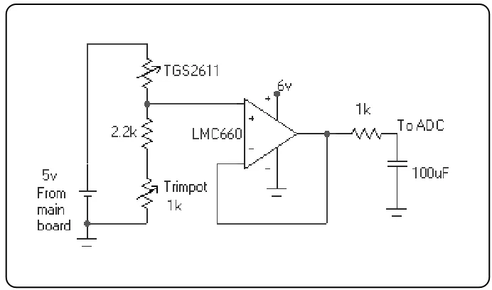
3.3.2.2 TGS2611 Methane Sensor

The TGS 2611 methane/ natural gas sensor varies in resistance logarithmically to

logarithmic gas concentrations between 500 and 10 000 ppm CH4, and is similarly

sensitive to H2. It requires a precision 5 V, 60 mA supply for its heater, again provided

by the main controller board by a separate 3 terminal regulator. The op-amp was

placed in a non-inverting arrangement, with unity gain. Being a resistive sensor, it was

placed in an adjustable voltage divider circuit, whose output was fed into the op-amp.

The resulting output voltage ranged from 0.39 to 2.67 V. The circuit is shown in Figure

(33)

[image:33.595.144.490.103.307.2]

3.4 Testing 21

Figure 3.6: TGS2611 CH4 sensor connections to LMC660CN op-amp.

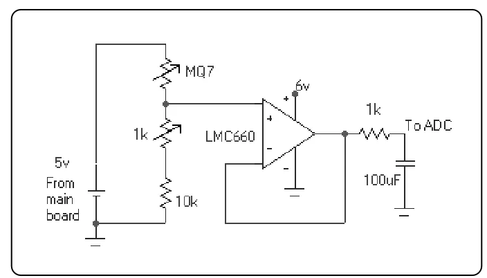
3.3.2.3 MQ7 Hydrogen Sensor

The MQ7 H2 sensor was the most complex to set up. Hanwei specifies a 150 second

heating cycle consisting of two precision heating voltages, the first being 5 V at 150

mA for 60 seconds, and the second 1.4 V at 43 mA for 90 seconds. This ruled out the

convenient use of 3 terminal regulators. Instead, one of the micro-controller’s timers

and PWM channels were used with a power MOSFET on the e-nose circuit board to

provide the required power and timing. The MQ7’s resistance varies logarithmically in

response to logarithmic gas concentrations up to 2000 ppm. The op-amp was set up

in a non-inverting configuration with a gain of 3, which saturated the op-amp during

practical trials detailed in chapter 5 The gain was then reduced to 2, which again led

to saturation. Unity gain finally resulted in an acceptable signal from 0.31 to 4.33 V.

The circuit is shown in Figure 3.7.

3.4

Testing

Trails with this e-nose arrangement consistently showed noisy readings. A sample of

such a signal is shown in Figure 3.8. Investigation with an oscilloscope lead to the

(34)

3.4 Testing 22

Figure 3.7: MQ7 H2 sensor connections to LMC660CN op-amp.

supply due to the switching of the serial communication and pulse-width modulation

(PWM) used to control the heater voltage of the H2 sensor. This is of little surprise as

no special precautions against noise were considered short of standard decoupling

ca-pacitors and minimal length circuit connections. The PWM spikes were approximately

0.03 V, considered acceptable and of little consequence due to compensation in the

micro-controller software described in Chapter 4, and serial communications are really

only necessary during software development, not during normal operation. The 50 Hz

noise was practically eliminated by choosing another power supply, and remaining noise

[image:34.595.140.492.99.300.2]

is considered negligible for the purposes of this project.

(35)

3.5

Chapter Summary

This chapter has detailed the components, and circuits in which they have been used,

as well as management, adjustments and precautions taken to assist effective function

throughout the development and testing phases of the system.

It will be seen in successive chapters how the signals obtained from these circuits are

used to indicate the composition of gas samples for the purpose of controlling digester

(36)

Chapter 4

Software

4.1

Chapter Overview

This chapter demonstrates the steps taken thoughout the software development process.

Three different control algorithms were considered during the initial stages of design.

The first was simple on-off control, commonly known as bang bang control, due to the

simple objectives of this project; to turn on or off a heater. Classical linear control

theory was also briefly considered, but dismissed due to the difficulty in modelling the

system due to the necessary number of inputs and the baffling number of variables

involved in the biological and physical aspects of the system.

Fuzzy logic control was chosen because of its inherent ability to deal with non-linear

systems, multiple inputs and noisy signals, with limited or unclear data available

re-garding the physical system. Prior expert knowledge may also be used as a starting

point to determine the behaviour of the system.

The hardware subroutines were based on examples provided by the avr-libc

documen-tation (Neswold 2006). The structure of the main program is a simple loop, the major

steps of which are illustrated by Figure 4.1. Implementation resulted in the files main.c,

adc.c, uart.c, timer.c and fuzzyfuncs.c, each so named to indicate the relevant device

(37)

ap-4.2 Implementation 25

pendices.

The program firstly reads the temperature and gas sensors, calculates averages to

re-move noise, then determines derivatives which are passed to the functionfuzzify();.

The fuzzified data is then de-fuzzified by the functiondefuzzify();to obtain a crisp

output which in this case, is an ideal target temperature intended to stimulate the

methanogenic bacteria to optimise CH4 production against digester heating

require-ments. This temperature setpoint is then compared to the actual digester temperature,

semaphore lights and heater being activated or de-activated accordingly.

4.2

Implementation

Initial efforts focussed on the reading of the ADC and placing the value in the USART.

This is initiated on the overflow of timer 1 in the micro-controller. Initial sampling time

periods during development were every half-second, but were scaled up to 2.5 minutes

in the working versions to suit the H2 sensor. The USART output consists of 8 bit data

words with 1 stop bit added at 2600 baud, which once converted to RS232 signal levels,

is readable by any serial communications terminal software, Minicom being used here.

The function void uart_put_num(float) was written to convert binary numbers to

ASCII words for sending over the USART for communication with a PC. One

short-coming of this subroutine is its inability to deal with floating point numbers, which

are simply converted to integers. This was used straight from the avr-libc examples

and the benefits not considered worth the time or memory necessary to rectify. The

implications of this will become apparent later in this chapter.

It was decided to use only the first derivatives as inputs to the controller so that rates of

change in gas concentration trigger responses. This eliminates the necessity of accurate

calibration of the equipment with respect to an absolute reference. Despite several

texts recommending the use of second derivatives, it was found that noise passed from

the gas sensors was too similar to the real second derivatives to be reliable.

(38)

4.2 Implementation 26

(39)

4.3 Fuzzy Control Software 27

the latest, as is common practice with computer systems. Cases were noted when

noisy signals resulted in incorrect derivative values over longer periods of time. This

was rectified by using buffer arrays to provide several consecutive readings. An running

average is then taken of the entire buffer and stored in a separate array of 3 consecutive

averages for each gas. While only 2 are necessary, a buffer of 3 allows for the calculation

of a second derivative if deemed useful later. Although this method slows the response

of the controller, it does significantly increase the reliability of detected changes in gas

concentrations over longer periods. It was found that buffer sizes of 6, 5 and 6 elements

provided adequately stable CO2, CH4 and H2 readings respectively, but these sizes can

easily be adjusted in the preprocessor#DEFINE GAS_buffer_sizelines as necessary.

4.3

Fuzzy Control Software

Fuzzy algorithms were based on Mamdani type fuzzy logic controller, originally

de-veloped by Doctor Lofti Zadeh and further dede-veloped by Professor Ebrahim

Mam-dani (Reznik 1997) and (Sowell 2005). The principles of their designs will be detailed

throughout this section. The functions are located in the file fuzzyfuncs.c.

Once readings from the ADC’s were being successfully read and sent to the USART, the

fuzzy logic functions were created to determine an acceptable temperature set point

be-tween the stated 21 and 38 degrees C using the centre of gravity (COG) method. These

were first implemented using MATLAB script and then ported to C. Additional

MAT-LAB script was developed to graphically display memberships and responses, which

greatly simplified the process of matching fuzzy logic parameters to sensors.

4.3.1 Fuzzifying

For the purpose of this system, a detected gas concentration or its derivative may be

regarded as low, medium or high. These are assigned based on prior expert knowledge

of the system and are known as membership functions. This expert knowledge may be

gained from a person familiar with the operating characteristics of the system to be

(40)

and 1 to each membership function, of which there may be as many as necessary to

achieve the desired control characteristics. It is common to have membership to more

than one membership function. This implementation monitors chosen variables and

assigns them a value of membership between zero and one to the membership functions

in the software ‘LOW’, ‘NORM’, and ‘HIGH’.

The exact assignment of a membership value is dependent on geometry built into the

system by the designer. For this implementation, LOWand HIGHare trapezoidal, while

NORM is triangular. These shapes were chosen due to their simplicity of

implemen-tation and simple area centroidal calculations. The positioning and dimensioning of

the geometry lies within the upper and lower expected extremities of the range of the

variable being monitored. This range is known as ‘the universe of discourse’ in fuzzy

terminology. The triangular geometry assigns a value which varies from 0 to 1 and

back to 0 again as an input value varies from the lower limits of what may be

consid-ered normal operating conditions. The trapezoids are suited to outer geometry in this

application, as they are able to assign membership for values of 1 outside the universe

of discourse, therefore maintaining control outside of normal operating ranges, while

gradually reducing membership as an input returns to normal. All geometry is set

by three, three-element arrays, ‘LOW_membs’, ‘NORM_membs’, and ‘HIGH_membs’ in the

program code. The first element of each array corresponds to the lowest point of the

geometry on the universe of discourse, the second element sets the centre point, and

the third element dictates the highest point of the geometry within the universe of

discourse.

These concepts are best illustrated by example. The arrays used in the initial MATLAB

scripts were as follows;

LOW_membs = [-16 -16 -2];

NORM_membs = [-16 0 10];

(41)

providing input membership functions which look like;

Figure 4.2: Controller initial input membership functions used to fuzzify.

with an input equal to zero, as indicated by circles plotted on each of the membership

functions. Here an input of zero returns a membership value of one for NORM, and zero

each for LOW and HIGH. Of importance in this example is the correlation between

the values within each array and the corresponding point along the corresponding

membership function.

Close inspection of the LOW and HIGH membership functions close to zero reveals

that membership to these functions does not occur until an input of -/+2 respectively.

This was done to provide immunity to noise, for reasons which will become clear later

in section 4.3.3.

The first element of theLOW_membs[]and the last of theHIGH_membs[]arrays are not

actually used by the fuzzy algorithms, they are only used in the MATLAB scripts to

determine the range of plots.

The code mechanisms used to arrive at a membership value are simply ‘if()’ tests

followed by statements consisting of linear equations of the formy=mx+c, or assign-ments of one or zero.

4.3.2 De-Fuzzify

The determined membership valuesLOW,NORMandHIGHare then used as the height in a

(42)

appro-4.3 Fuzzy Control Software 30

priate responses such as ‘increase temperature’, ‘maintain temperature’, or ‘decrease

temperature’. Obviously this has a direct impact on the magnitude and distribution

of area, and therefore the position of the centroid, which is how the temperature set

point is calculated. This is the principle of Mamdani’s fuzzy controller. The centroid

is calculated using equation 4.1 where An is nth area, zn is the centroid of the nth

area, and cn is a scalar weighting constant of the nth input. This allows a designer

to emphasise the influence of a particular input over the others. It may be observed

that the formula lends itself well to expansion to include multiple response areas. This

allows simple monitoring of multiple inputs to determine a single output.

Z = Pn

n=1cnAnzn

Pn

n=1cnAn

(4.1)

The Mamdani fuzzy logic process is not easy to visualise through literature. Plots in

Figures 4.3 to 4.7 below show the fuzzification and defuzzification and thus response of

the controller to several progressive values of the first derivative of CO2.

As is the case with the input membership functions, the response geometry is set in the

arrays ‘DN_TEMP_membs’, ‘AB_RITE_membs’ and ‘UP_TEMP_membs’, which are included

below as implemented in MATLAB script. The upper plot in each of these figures

illustrates the membership value for each input function and is plotted as a small

circle, consistant with Figure 4.2. The lower plots show the response functions and the

temperature set point. Note that the height of each response area is dependent on the

value of the membership value of the corresponding input membership function. It is

the sum of these areas for which the centroid determines the set point.

CO2 input: CO2 output:

CO2_LOW_membs = [-16 -16 -2]; CO2_DN_TEMP_membs = [15 15 35];

CO2_NORM_membs = [-16 0 10]; CO2_AB_RITE_membs = [25 30 37];

CO_2HIGH_membs = [ 2 10 16]; CO2_UP_TEMP_membs = [29 39 45];

Figure 4.3 shows the controller’s response to an input outside the universe of discourse.

Notice that the temperature setpoint will never recede below the the COG of the

(43)

−200 −15 −10 −5 0 5 10 15 20 0.2

0.4 0.6 0.8 1

Input Membership Functions

LOW NORM HIGH d GAS/ dt

15 20 25 30 35 40 45

0 0.5 1

Response

Temperature Set Point

dn temp ab rite up temp centroid

Figure 4.3: Controller response to an input of -20.

−200 −15 −10 −5 0 5 10 15 20 0.2

0.4 0.6 0.8 1

15 20 25 30 35 40 45

0 0.2 0.4 0.6 0.8 Response

Figure 4.4: Controller response to an input of -10.

Figure 4.4 depicts the input value rising to -10. Notice that the input has now been

assigned membership to two functions, LOW and NORM. These determine the height of

the DN_TEMP and AB_RITE triangles, the areas of which are summed and the COG

(44)

−200 −15 −10 −5 0 5 10 15 20 0.2

0.4 0.6 0.8 1

15 20 25 30 35 40 45

0 0.5 1

Response

Figure 4.5: Controller response to an input of 0.

Figure 4.5 exhibits the selected ideal operating point of the digester. Small fluctuations

of up to±2 in input will not affect the setpoint, as theDN_TEMPandUP_TEMP response

triangles have a height of 0.

−200 −15 −10 −5 0 5 10 15 20 0.2

0.4 0.6 0.8 1

Input Membership Functions LOW

NORM HIGH d GAS/ dt

15 20 25 30 35 40 45

0 0.1 0.2 0.3 0.4 Response

Temperature Set Point dn temp

ab rite up temp centroid

(45)

The response of the controller to an input of +5 is shown in Figure 4.6. Membership

to input function NORMand HIGHdetermine height of AB_RITE and UP_TEMP response

triangles.

Figure 4.7 depicts the response of the controller to an input exceeding the universe of

discourse. Again, temperature setpoint cannot exceed the upper limit of the COG of

theUP_TEMP response triangle.

−200 −15 −10 −5 0 5 10 15 20 0.2

0.4 0.6 0.8 1

Input Membership Functions LOW

NORM HIGH d GAS/ dt

15 20 25 30 35 40 45

0 0.5 1

Response

Temperature Set Point dn temp

ab rite up temp centroid

Figure 4.7: Controller response to an input of +20.

4.3.3 Tuning Fuzzy Parameters

Mentioned in the previous section is the point that expert knowledge of a physical

system may be used to set the fuzzy parameters. These parameters are present in the

*_membs[]arrays declared in the main file. Six of these must be declared for each gas,

three each for input and output. The program requires values which form trapezoids for

two outer membership functions and triangles for those in the centre. The temperature

set point for the range of expected inputs or universe of discourse, in this case the first

(46)

−200 −15 −10 −5 0 5 10 15 20 0.2

0.4 0.6 0.8 1

1st Derivative CO2

LOW NORM HIGH

−20 −15 −10 −5 0 5 10 15 20 20

25 30 35 40

Response

1st Derivative CO2

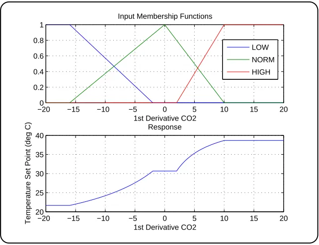
[image:46.595.158.479.104.351.2]

Temperature Set Point (deg C)

Figure 4.8: Temperature set point for expected d(CO₂)/dt levels.

Of interest are the slopes either side of the above-mentioned dead zone either side of

inputs of zero, for two reasons, which will now be discussed.

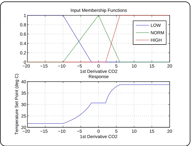
4.3.4 Slope

The first reason for interest in these two slopes may have already been noticed; the

gradient influences the magnitude of the response, which in this case, is the magnitude

of the change in temperature setpoint for a given change in input. Figure 4.9 shows an

experiment with this relationship using the following input membership arrays:

LOW_membs = [-16 -10 -2];

NORM_membs = [-10 0 6];

HIGH_membs = [2 6 16];

Comparing Figure 4.9 with 4.8, it may be appreciated while steeper gradient has the

effect of increasing the magnitude of the response over small fluctuations in input, it also

(47)

−200 −15 −10 −5 0 5 10 15 20 0.2

0.4 0.6 0.8 1

1st Derivative CO2

LOW NORM HIGH

−20 −15 −10 −5 0 5 10 15 20 20

25 30 35 40

Response

1st Derivative CO2

[image:47.595.158.481.103.349.2]

Figure 4.9: Modified Temperature set point for expected d(CO₂)/dt levels.

4.3.5 Concavity

Secondly, while the profile of Figure 4.8 could well result in a functional controller, the

concavity of these two curves means that temperature set point adjustments are smaller

close to the upper and lower limits of the operating temperature range. Conversely,

responses are more dramatic close to the centre flat spot. This situation means that

for small inputs outside the dead zone, more dramatic adjustments are made.

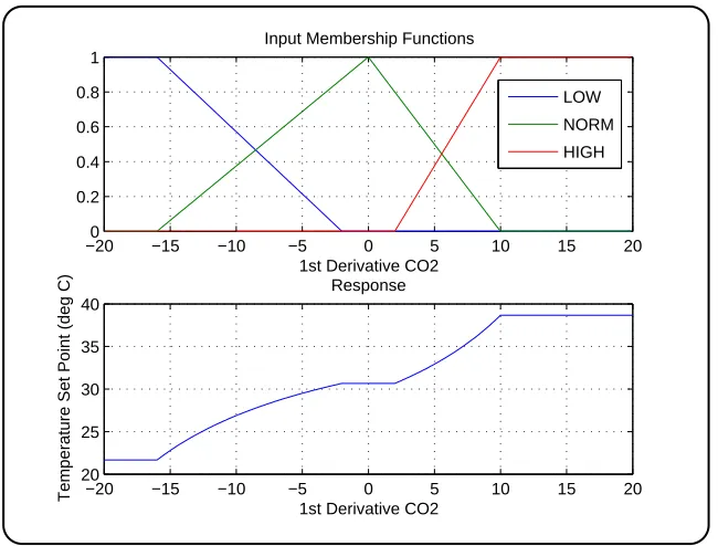
Great advantage may be taken of this characteristic. As it is more likely that readings

close to zero may be caused by noise, an alternative was investigated by altering

pa-rameters in the*_membsarrays to reverse the concavity of these two areas as in Figure

4.10. This has the effect of triggering smaller adjustments in set point close to zero,

which are likely to be noise, while readings further from this region will trigger more

dramatic responses, where they are more necessary.

Figure 4.10 was created by widening the base of theAB_RITE response triangle by

ini-tialising array AB_RITE_mems = [10 30 52]. Further adjustments to input functions

(48)

4.4 Micro-controller Implementation 36

−200 −15 −10 −5 0 5 10 15 20 0.2

0.4 0.6 0.8 1

1st Derivative CO2

LOW NORM HIGH

−20 −15 −10 −5 0 5 10 15 20 20

25 30 35 40

Response

1st Derivative CO2

[image:48.595.157.482.103.350.2]

Figure 4.10: Modified temperature set point for expected d(CO₂)/dt levels.

Further exploration into the effects of various membership function shapes are thought

to be of limited additional benefit to this project and so are left as specific areas worthy

of curiosity and nothing more.

4.4

Micro-controller Implementation

Once the MATLAB routines were ported to C, experimentation with the micro-controller

could begin. Minicom was used to capture ASCII text in data files which were then

(49)

4.4 Micro-controller Implementation 37

0 5 10 15 20 25 30 35 40

−30 −20 −10 0 10 20 30

CO2: 1st Derivative

Sample No

d(CO2/dt)

−20 −15 −10 −5 0 5 10 15 20 20

30 40

d(CO2)/dt vs Temp Setpoint

Temp SP (deg C)

[image:49.595.159.481.103.348.2]

d(CO2)/dt

Figure 4.11: Captured temperature set point for expected d(CO₂)/dt levels.

0 5 10 15 20 25 30 35 40

−30 −20 −10 0 10 20 30

CO2: 1st Derivative

Sample No

d(CO2/dt)

−20 −15 −10 −5 0 5 10 15 20 20

30 40

d(CO2)/dt vs Temp Setpoint

Temp SP (deg C)

d(CO2)/dt

Figure 4.12: Captured modified temperature set point for expected d(CO2)/dt levels.

It is here that the limitations of the simple function void uart_put_num(float)

be-come apparent. However a clear correlation between the plots in Figures 4.11 and 4.8,

[image:49.595.159.479.393.636.2]

(50)

4.5

Chapter Summary

This chapter has detailed the process of software development for the fuzzy logic

con-troller for a biogas system. The process has been illustrated using examples from the

first derivative of CO2 readings. Changes to the gradient of the controller’s response

and the ease with which parameters may be adjusted to suit sensor response

character-istics leads to the conclusion that this procedure may be followed to develop suitable

(51)

Chapter 5

Laboratory Gas Tests

5.1

Chapter Overview

This section explains the equipment and process used to test the response of the sensors

to expected gas concentrations and levels. The data is required to tune fuzzy parameters

to individual sensors. It concludes with comments regarding the suitability of the

signals for use with thefuzzify()and defuzzify()functions.

5.2

Test Equipment

The necessary function of the sampling equipment is to precisely dilute a gas sample

to a known concentration and expose the sensors to a consistant concentration for a

period long enough to allow the sensors to respond.

Hypodermic syringes of 6 and 3 mL volume were used to take accurately measured gas

samples. Considering the implications of 1mL variation in volumes of the sample gas

and air with which to dilute the samples, accurate measuring of air was not considered

so crucial as precision. A plastic 600 ml bottle was cleaned and pierced on the bottom

to provide a snug fit for the syringes, one of which was then inverted and inserted

(52)

5.3 Sampling Procedure 40

consitant volumes, gas samples could be diluted with sufficient precision to a desired

concentration for analysis.

A sketch of the essential components of the apparatus is shown in Figure 5.1. Arrows

[image:52.595.230.407.205.524.2]

indicate the direction of applied force during a dilution operation.

Figure 5.1: Dilution equipment used throughout laboratory tests.

Pure test gas samples of CO2 and H2 were provided by the USQ Faculty of Sciences,

but CH4 was not available and so was substituted with town gas. Australian

Stan-dard 4564-2000 is somewhat arbitrary with constituent components of natural gas, the

implications of which become clear in later in Section 5.4.

5.3

Sampling Procedure

Having two known volumes allowed gas concentration to be determined using the

(53)

5.3 Sampling Procedure 41

V OLU M Esyringe=

V OLU M Ebottle×CON CEN T RAT ION(ppm)

106 (5.1)

Where V OLU M Ebottle = 600 mL, and CON CEN T RAT ION is the concentration

desired.

To sample a gas, a syringe was placed on the outlet of the gas regulator without the

plunger and thoroughly purged. The plunger was then replaced and inserted to give

the calculated volume,V OLU M Esyringe at a positive pressure.

The syringe was then quickly inserted into the hole in the base of the 600 mL bottle

which was raised slightly to give a negative pressure. The syringe plunger was then

depressed into the bottle until empty and the bottle raised to its maximum height in the

water. The breach was then covered and great care was taken to ensure the mouth of

the bottle remained below the waters surface at a consistant level. The gas sample may

then be considered diluted to the greatest precision available under the circumstances.

To test the sample, the inverted pill bottle and sensors were placed above the hole and

the 600 mL bottle pushed gently and consistently downward so that the diluted gas

entered the sensor chamber. The cap was then promptly replaced and the equipment

allowed to sit for analysis.

5.3.1 Microcontroller Configuration

As mentioned in Chapter 3, the MQ7 H2sensor requires a 150 second heating cycle. The

timer interrupt subroutine was altered to provide the necessary sensor heating states

over the required time period. Buffers were implemented as described in Chapter 4.

Raw readings, averages and first derivatives were sent via the serial port and captured

(54)

5.4 Testing 42

5.4

Testing

Unfortunately time constraints permitted only 3 useful tests, each of a single sample.

The details of these are listed below.

• Trial 1: 10 000 ppm CO2

• Trial 2: 1 000 ppm H2

• Trial 3: 10 000 ppm town gas

From these it was expected that an algorithm based on 3 linear equations could be

derived to extract individual gas concentrations, which could then be sent to the fuzzy

functions to derive a temperature setpoint.

Plots in Figures 5.2 to 5.10 show the data captured in the trails. The horizontal

axis represents the sample number, or time in increments of 150 s, while the vertical

axes represent the voltage captured by the micro-controller’s ADC’s. Apparent lags in

averages and derivatives are a result of updates in buffer arrays. Captured data files

are included in Appendix C.

5.4.1 Trial 1

Figures 5.2 to 5.4 show data captured in trial 1.

Inspection of these plots show a dramatic response from the CO2 sensor, with only

a slight, but noisy response from the CH4 sensor, and what may be interpreted as

background noise from the H2 sensor. Having replaced the noisy power supply, the

source of this noise is unknown, it is thought that it may be a characteristic of the

sensors’ cross-sensitivity, or fluctuations in air quality in the laboratory, as USQ staff

were cleaning and preparing equipment on the day. This aside, the result was very

encouraging, as it appears that CO2 levels affect the other sensors minimally. It can be

seen in the centre plots that the averaging algorithms remove the spikes to an acceptable

(55)

5.4 Testing 43

0 5 10 15 20 25 30 35 40

0 100 200

CO2

0 5 10 15 20 25 30 35 40

0 100 200

CO2 averaged

0 5 10 15 20 25 30 35 40

−50 0 50

[image:55.595.159.480.104.347.2]

CO2: 1st Derivative

Figure 5.2: Captured data from CO₂ sensor; trial 1.

0 5 10 15 20 25 30 35 40

60 80 100

CH4

0 5 10 15 20 25 30 35 40

70 80 90

CH4 averaged

0 5 10 15 20 25 30 35 40

−5 0 5

CH4: 1st Derivative

Figure 5.3: Captured data from CH4 sensor; trial 1.

5.4.2 Trial 2

Trial 2 as defined here did not run as smoothly as expected due to excessive gain in

[image:55.595.159.479.390.636.2]

(56)

5.4 Testing 44

0 5 10 15 20 25 30 35 40

150 200 250

H2

0 5 10 15 20 25 30 35 40

150 200 250

H2 averaged

0 5 10 15 20 25 30 35 40

−10 0 10

[image:56.595.159.481.104.350.2]

H2: 1st Derivative

Figure 5.4: Captured data from H₂sensor; trial 1.

as anticipated, yielding the plots 5.5 to 5.7.

0 5 10 15 20 25

0 50 100

CO2

0 5 10 15 20 25

0 20 40

CO2 averaged

0 5 10 15 20 25

−20 0 20

CO2: 1st Derivative

Comparing Figures 5.5 and 5.7, it appears from trial 2 plots that H2 appears to affect

the CO2 sensor noticeably, but not excessively. This is unexpected as the MG811

[image:56.595.160.479.426.671.2]

(57)

5.4 Testing 45

0 5 10 15 20 25

0 200 400

CH4

0 5 10 15 20 25

0 100 200

CH4 averaged

0 5 10 15 20 25

−50 0 50

[image:57.595.159.480.104.348.2]

CH4: 1st Derivative

Figure 5.6: Captured data from CH₄ sensor; trial 2.

0 5 10 15 20 25

0 500 1000

H2

0 5 10 15 20 25

0 500 1000

H2 averaged

0 5 10 15 20 25

−200 0 200

H2: 1st Derivative

Figure 5.7: Captured data from H2sensor; trial 2.

also significantly affected, and this is noted in the TGS2611 datasheet. Looking at

the derivative plots, both of these signals are clearly unable to be concealed by simple

noise allowance techniques covered in Chapter 4, indicating some kind of compensation

[image:57.595.159.479.391.636.2]

(58)

5.4 Testing 46

5.4.3 Trial 3

Trial 3 also suffered from complications, but this time the major source is uncertainty

in town gas composition.

Plots are shown in Figures 5.8 to 5.10.

0 5 10 15 20 25 30 35 40

0 20 40

CO2

0 5 10 15 20 25 30 35 40

0 20 40

CO2 averaged

0 5 10 15 20 25 30 35 40

−10 0 10

[image:58.595.159.481.228.470.2]

CO2: 1st Derivative

It is clear that all 3 sensors have again reacted to town gas, but is unclear at this point

as to exactly why. It appears the CO2 sensor’s response closely resembles that in trial

2. The CH4 sensor has also reacted strongly, as should be expected due to the high

percentage of CH4 in town gas. The H2 sensor has also reacted strongly.

Unfortunately no gas spectrum analyser was available, so it is unclear to exactly what

these responses may be attributed, and to what degree it/ these affect each sensor. The

Australian Government (Roarty 1998) suggests that natural gas may contain propane,

C3H8 and butane C4H10, which are the major constituents of liquefied petroleum gas

(LPG). Australian Standard 4564-2000 does not impose limits on the composition of

natural gas for consumption; only a minimum calorific combustion value known as the

Wobbe Index of between 46 and 52 MJ/m3

. Hanwei inform that the MQ7 H2 sensor is

(59)

5.4 Testing 47

0 5 10 15 20 25 30 35 40

0 500 1000

CH4

0 5 10 15 20 25 30 35 40

0 500 1000

CH4 averaged

0 5 10 15 20 25 30 35 40

−100 0 100

[image:59.595.159.481.105.349.2]

CH4: 1st Derivative

Figure 5.9: Captured data from CH₄ sensor; trial 3.

0 5 10 15 20 25 30 35 40

0 500 1000

H2

0 5 10 15 20 25 30 35 40

0 500

H2 averaged

0 5 10 15 20 25 30 35 40

−100 0 100

H2: 1st Derivative

Figure 5.10: Captured data from H2 sensor; trial 3.

Additionally, it may be expected that in the presence of such a confused array of

hydrocarbon gases, the MQ7 may also be affected by other gases present, one of which

could well be free H2. In the absence of any information, excluding the datasheet, it is

[image:59.595.159.479.390.634.2]

(60)

5.5 Chapter Conclusion 48

The significance of this assumption will become clear in Chapter 6.

Similar conclusions may be drawn regarding the response of the CO2 sensor. It is

known that town gas does contain CO2, but it is uncertain in what quantity, and it is

also unknown to what degree the sensor is affected by other gases.

5.5

Chapter Conclusion

This chapter has detailed and commented on the equipment and procedure to test the

responses of the sensors to expected gas composition.

On cursory inspection, it may appear that the unravelling of this data to provide

useful information concerning individual gas concentrations, as proposed earlier in this

dissertation, means that significant further work is necessary in this area, and this is

indeed the subject of a great deal of recent research.

For the purpose of this project, two points must be highlighted. The first is that the

method used to gather this data is highly inconsistent in nature due to the sudden

expos

Embedded control system for biogas digesters

University of Southern Queensland

Certification of Dissertation

Acknowledgments

Contents

List of Figures

Chapter 1

Objectives

Methodology

Chapter 2

Biogas Production

Digester Control

Safety Considerations

Chapter Summary

Electronic Hardware

Microcontroller

E-nose

Testing

Chapter Summary

Chapter 4

Implementation

Fuzzy Control Software

LOW NORM HIGH

LOW NORM HIGH

LOW NORM HIGH

Micro-controller Implementation

Chapter Summary

Chapter 5

Test Equipment

Sampling Procedure

Testing

Chapter Conclusion