Analytical study on the influence of distributed beam vertical loading on seismic response of frame structures

City, University of London Institutional Repository

Citation

:

This is the accepted version of the paper.

This version of the publication may differ from the final published

version.

Permanent repository link:

Link to published version

:

Copyright and reuse:

City Research Online aims to make research

outputs of City, University of London available to a wider audience.

Copyright and Moral Rights remain with the author(s) and/or copyright

holders. URLs from City Research Online may be freely distributed and

linked to.

City Research Online: http://openaccess.city.ac.uk/ [email protected]

Analytical study on the influence of distributed beam

vertical loading on seismic response of frame structures

P.E. Mergos*1a _{and A.J. Kappos}1b

1_{City University London, School of Engineering and Mathematical Sciences, Department of Civil Engineering,}

London EC1V 0HB, United Kingdom

Abstract. Typically, beams that form part of structural systems are subjected to vertical distributed loading along their length. Distributed loading affects moment and shear distribution, and consequently spread of inelasticity, along the beam length. However, the finite element models developed so far for seismic analysis of frame structures either ignore the effect of vertical distributed loading on spread of inelasticity or consider it in an approximate manner. In this paper, a beam-type finite element is developed, which is capable of considering accurately the effect of uniform distributed loading on spreading of inelastic deformations along the beam length. The proposed model consists of two gradual spread inelasticity sub-elements accounting explicitly for inelastic flexural and shear response. Following this approach, the effect of distributed loading on spreading of inelastic flexural and shear deformations is properly taken into account. The finite element is implemented in the seismic analysis of reinforced concrete (R/C) frame structures with beam members controlled either by flexure or shear. It is shown that to obtain accurate results the influence of distributed beam loading on spreading of inelastic deformations should be taken into account in the inelastic seismic analysis of frame structures.

Keywords: seismic analysis; finite element; distributed inelasticity; beam members; distributed loading.

1. Introduction

In recent years, nonlinear analysis procedures, although more complex and computationally demanding, have gained favour over the conventional linear elastic methods for the seismic analysis of structures. This is the case because they model realistically structural response and provide reliable and accurate analytical predictions. Nevertheless, the inherent assumptions of these procedures may, in some cases, jeopardize their credibility and drive the analysis to erroneous results.

It is well known that beam members are subjected to distributed vertical loading along their length. Beam distributed loading arises from the supported slab area distributed loads, the overlying infill walls, and beam self-weight. Distributed loading generates nonlinear bending moment diagrams and variation of the acting shear forces along the member length.

In the vast majority of inelastic seismic analyses, beam distributed loading is either ignored or treated in an approximate manner. Typically, end-moments arising from distributed loading are added to the seismic end-moments, but the moment diagram is assumed to be linear and the acting shear force constant along the beam length. This approach originates from the assumption that under a strong earthquake, distributed

loading moments and shears represent a negligible fraction of the respective seismic demand. However, this is not the actual situation in a number of cases arising in real structures. This is particularly the case in buildings with long-span beams and/or heavy slabs and infill walls, and in all buildings subjected to low seismic actions, especially in their upper floors. The significance of accurately modelling the effect of distributed beam loading on spreading of inelastic flexural and shear deformations increases if one considers the fact that capacity design principles, adopted by all modern seismic design guidelines, dictate development of plastic hinges at the beam ends, so that a beam-sway mechanism develops and a soft-storey mechanism is prevented.

The above remarks point to the need for a finite element capable of consistently modelling distributed beam loading effects in inelastic seismic analysis of structures. A large number of finite element models of the beam-column type have been proposed for inelastic seismic analysis of frame structures. The most common and widely used ones are the concentrated (lumped) plasticity models (Clough and Johnston 1966; Giberson 1967). These models, while computationally attractive, may yield inaccurate predictions because the assumed inelastic zone length is in reality a function of the boundary conditions and member moment distribution (Anagnostopoulos 1981).

In recent years, flexural force-based distributed finite elements (Spacone et al. 1996; Neuenhofer and Filippou 1997) have gained favour, because this approach provides fairly accurate prediction of inelastic response with a single element discretization of the structural member. Moreover, a number of these elements have been enhanced to account for shear flexibility (Ceresa et al. 2007). Nevertheless, distributed inelasticity elements using Gauss or Gauss-Lobatto integration techniques are not computationally efficient for members with inelastic deformations only at their ends (Lee and Filippou 2009), as the case typically is with seismic loading. In this case, the aforementioned finite elements behave like an element with an inelastic zone of fixed length at each end, if only the integration point closest to the end of the member experiences yielding (Lee and Filippou 2009). The length of the inelastic zone equals the integration weight of the end monitoring section. Increasing the number of integration points is computationally inefficient, unless the element is subdivided into an inelastic region at each end and an intermediate elastic region (Addessi and Ciampi 2007). Even so, it is possible that only the integration point closest to the end experiences plastic deformations, particularly for small strain hardening ratios (Lee and Filippou 2009).

Lee and Filippou (2009) compared the performance of conventional distributed inelasticity force-based elements applying the Gauss-Lobatto integration technique and that of a new finite element with variable inelastic end-zones (named SIZE model) proposed in their study. They found that under double curvature conditions (typical case under seismic loading), the distributed inelasticity element with 5 fixed integration points may lead to significant deviations from the exact solution. On the other hand, the SIZE model was found to provide very good convergence with less computational cost. To achieve the same level of accuracy, 10 equal-length finite elements with 5 Gauss-Lobatto integration points were applied by these researchers for the structural member under investigation.

present, the bending moment diagram decreases from the support to the mid-span more rapidly in the hogging moment region and less rapidly in the sagging moment region, compared to the case that there is no distributed loading (which is never true for beams). Hence, for the same end moments (controlled by the member’s flexural capacity), the length of the inelastic end zone becomes smaller for hogging moments and larger for sagging moments with respect to the zero distributed loading case. As a result, the possibility that only the integration point closest to the end experiences plastic deformations increases for the end with hogging moment and decreases for the

end with sagging moment. Both these effects of distributed vertical loading are

further explained in the remainder of the paper.

Furthermore, for these conventional distributed inelasticity elements incorporating shear flexibility, the lengths of the flexural and shear inelastic end regions are restricted to be identical and equal to the integration weight of the monitoring section. Hence, the possibility that the inelastic flexural and shear deformations expand along different lengths due to the different moment and shear force variation along the structural member cannot be modelled explicitly by these elements.

To capture the gradual spreading of inelastic deformations, a spread inelasticity formulation with variable length inelastic zones is needed. Several research studies have introduced such flexural inelasticity elements. Meyer et al. (1983), Reinhorn et al. (2009), Lee and Filippou (2009) and Roh et al. (2012) proposed flexural gradual spread inelasticity models, which ignore influence of distributed loading. Soleimani et al. (1979) and Filippou and Issa (1988) suggested similar flexural spread inelasticity beam models, where distributed loading is taken into account approximately by assuming constant shear force in the plastic hinge regions. Kyakula and Wilkinson (2004) proposed a flexural spread plasticity model, where the inelastic zones ends are determined by linear interpolation between fixed monitoring sections, where differences between acting and yielding moments change sign. This approach may take into account the influence of distributed loading. Nevertheless, it is an approximate method and it may require a significant number of monitoring sections. None of the aforementioned gradual spread inelasticity elements, apart from the model of Roh et al. (2012), considers variation of shear flexibility along beam members.

Mergos and Kappos (2009, 2012) developed a shear spread inelasticity model to capture shear-flexure interaction effect for R/C members with constant shear force. The model assumes inelastic shear end zones with variable length defined by the respective zones of the flexural sub-element. A similar approach has been adopted by Roh et al. (2012).

Furthermore, in an earlier work (Mergos and Kappos 2008), the authors introduced the concept of a shear spread plasticity model which captures variation of shear flexibility, when distributed loading is present and acting shear varies along the member length. However, since this analytical work focussed on shear-flexure interaction of single R/C column members, the complete formulation of the proposed model to account for the beam distributed loading effect on spreading of both inelastic flexural and shear deformations was not developed. Moreover, the analytical model was not applied in seismic analysis of beam members with distributed loading.

extended to cope with different types of vertical loading. The analytical model formulation is described in detail, together with its inherent assumptions. Finally, the analytical model is implemented in a computer code for inelastic static and dynamic analysis and applied to plane frames with different configurations. Useful conclusions are drawn regarding the influence of beam vertical loading on seismic response of R/C frame structures.

2. Finite Element Model Formulation

2.1 General description

The proposed, member-type, finite element is based on the flexibility approach (force-based element) and belongs to the class of phenomenological models. It consists of two sub-elements representing flexural and shear element response (see Fig. 1). The total flexibility matrix [F] is calculated as the sum of the flexibilities of its sub-elements and can be inverted to produce the element stiffness matrix [K]; hence:

 

    (1)

where, [F], [Ffl], [Fsh] are the basic total, flexural, and shear, respectively, tangent flexibility matrices. [K] is the basic tangent stiffness matrix of the element, relating incremental moments ΔΜΑ, ΔΜΒ and rotations ΔθΑ, ΔθΒ at the ends A and B of the

flexible part of the element (Fig. 1).

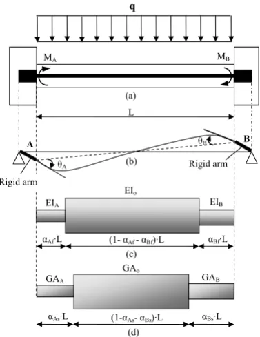
The flexural sub-element is used for modelling flexural behaviour of the beam member subjected to cyclic loading before, as well as after, flexural yielding. It

consists of a set of rules governing the hysteretic moment-curvature (M-φ) behaviour

of the member end sections, and the flexural spread plasticity model. The flexural spread plasticity model is composed of the model for flexural stiffness distribution and the model for determination of the variable length of the inelastic flexural end-zones.

The shear sub-element is defined in the same way as its flexural counterpart. It is determined by a set of rules governing the hysteretic shear force vs. shear distortion

(V-γ) behaviour of the member end sections and the shear spread plasticity model; the

latter is composed of the model for shear stiffness distribution and the model for defining the variable length of the inelastic shear end-zones.

Due to their similarity, the individual components of the flexural and shear sub-elements are developed in parallel in the following sections. Analytical model assumptions and limitations are also discussed.

Figure 1: Proposed finite element model: a) geometry of R/C beam member with distributed vertical loading; b) beam finite element with rigid offsets; c) flexural sub-element; d) shear sub-element

2.2 End-section hysteretic relationships

An appropriate M-φ and V-γ hysteretic model is applied to determine the hysteretic

response of end-sections of the flexural and shear sub-element, respectively. These hysteretic models are described by the primary (skeleton) curve and the rules determining section response under cyclic loading.

In this study, it is assumed that envelope M-φ and V-γ responses can be adequately

approximated by a bilinear skeleton curve (Fig. 2). This skeleton curve consists of an elastic and a post-elastic linear branch separated at the level of flexural My or shear

yielding Vy. Furthermore, it is assumed herein that shear yielding is independent of

flexural yielding and vice versa. The latter assumption may not be accurate for some classes of structural members like for example shear-flexure critical RC members (Mergos and Kappos 2012). Nevertheless, for the vast majority of structural members, especially those designed according to modern seismic design principles, shear-flexure interaction maybe disregarded with reasonable accuracy (Lehman and Moehle 1998; Beyer et al. 2011).

Figure 2: M-φ (V-γ) sub-element end-section hysteretic models

ΜA ΜΒ

θA

θΒ

L

ΕΙΑ

ΕΙο

ΕΙΒ

GAΑ

GAo

GAB (a)

(b)

(c)

A

Rigid arm

Rigid arm

B

q

αΑf·L (1- αΑf - αBf)·L αBf·L

(d)

αΑs·L (1-αΑs- αBs)·L αBs·L

φ (γ) M (V)

1 2,8 9,17

18

My+(V y+)

3

4 6

14,16

13 10 12

11

My-(V y-)

7 15 0

The multi-linear, ‘yield-oriented’ with slip, hysteretic model of Sivaselvan and

Reinhorn (2000) is adopted herein for describing M-φ and V-γ cyclic behaviour. This

model accounts for stiffness degradation, strength deterioration, pinching effect and non-symmetric response. However, its original formulation is based on a trilinear envelope curve. Hence, its hysteretic rules were appropriately modified by the authors (Mergos and Kappos 2008) to make them compatible with a bilinear skeleton curve. In general, different hysteretic parameters are applied to describe hysteretic flexural and shear response.

2.3 Stiffness distribution

To capture the current distribution of section flexural and shear stiffness along the beam, a gradual flexural and shear, respectively, spread inelasticity model is assigned (Soleimani et al. 1979; Mergos and Kappos 2008, 2012). Following this model, each sub-element is divided into two inelastic end-regions and one elastic intermediate zone.

Inelastic end-zones determine the part of the flexural or shear sub-element where flexural or shear yielding, respectively, have occurred. The length of these inelastic zones generally varies throughout member response and the way it is defined at each analysis step is described in the following sections.

Stiffness along the intermediate zone is assumed to be constant and equal to the

elastic stiffness EIo of the end-section M-φ envelope curve for the flexural

sub-element and GAo of the end-section V-γ envelope curve for the shear sub-element. If

the elastic stiffnesses of the two end-sections are different, then an average value is assigned to the intermediate zone (Eq. 2) as also suggested by Reinhorn et al. (2009),

where EIoA, EIoB, GAoA, GAoB are the elastic stiffnesses at the ends A and B

respectively.

2 _{oA oB}

o

oA oB

EI EI

EI

EI EI

 



 ;

2 _{oA oB}

o

oA oB

GA GA

GA

GA GA

 



 (2)

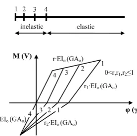
Stiffness distribution within the inelastic zones depends on the loading state of the end section hysteretic response. In particular, Fig. 3 illustrates hysteretic response of four cross-sections located inside one region of the flexural (shear) sub-element. It can be seen that when all sections remain on the strain hardening branch (loading state),

flexural (shear) stiffness remains constant in the inelastic zone and equal to r·EIo

(r·GAo) (0<r<1).

However, when the end sections are in the unloading and reloading state, stiffness varies from a minimum value r1·EIo (r1·GAo) and r2·EIo (r2·GAo) (0<r1,r2<1)

corresponding to the end section, to a maximum value, which is equal to EIo (GAo).

Hence, under the general assumption that the loading state of all sections of the

yielded region remains the same, it can be considered that when M-φ (V-γ) end

section hysteretic response is on the strain hardening branch, stiffness distribution

remains uniform in the inelastic zone. In the case where end-section M-φ (V-γ)

Figure 3. M-φ (V-γ) hysteretic response of cross-sections inside a plastic hinge

In line with the previous observations, stiffness distribution along the member may be assumed to have one of the shapes shown in Fig. 4, where L is the length of the

member; EIo (GAo) is the stiffness in the intermediate part of the element and EIA

(GAA) and EIB (GAB) are the current tangent flexural (shear) rigidities of the sections

at the ends A and B respectively. The flexural (shear) rigidities EIA (GAA) and EIB

(GAB) are determined by the M-φ (V-γ) hysteretic relationships of the corresponding

end sections. Similar assumptions are made by Soleimani et al. (1979) and Roh et al. (2012).

Nevertheless, it should be kept in mind that these assumptions remain a compromise between the need for low computational cost, as assured by the use of only two monitoring end-sections, and the need for accurate representation of the stiffness distribution along the member length. The validity of these assumptions increases as the length of the inelastic zones decreases (Soleimani et al. 1979). Hence, for the typical cases of seismic response, where the lengths of the inelastic zones remain relatively small, the aforementioned assumptions are deemed as adequate.

Figure. 4. Element stiffness distribution: (a) when ends A and B are in the loading state; (b) when ends A and B are both in the unloading or reloading state; (c) when end A is in the loading and end B is in the unloading or reloading state; (d) when end A is in the unloading or reloading state and end B is in the loading state

inelastic 2

1 3 4

1

4 3 2 1 φ (γ)

Μ (V)

EIo (GAo)

r1·EIo (GAo)

r2·EIo (GAo) r·EIo (GAo)

0<r,r1,r2≤1 4 3 2

elastic

Α

Β EIo (GAo)

EIA (GAA) EIB (GAB)

αAL (1-αA- αΒ)L αΒL

αAL (1-αA- αΒ)L αΒL a)

b)

αAL (1-αA- αΒ)L

αAL (1-αA- αΒ)L

L

c)

d)

αΒL

αΒL

Α Β

Β Α

Α Β

EIA (GAA)

EIA (GAA)

EIA (GAA)

EIB (GAB) EIB (GAB)

EIB (GAB) EIo (GAo)

EIo (GAo)

2.4 Inelastic end-zone lengths

In Fig. 4, αA and αB are the inelastic zone coefficients. The inelastic zone coefficients

specify the proportion of the member that has yielded either in flexure (αAf and αBf) or

in shear (αAs and αBs). By definition, αAf and αBf represent the part of the flexural

sub-element, where acting moment exceeds section yield moment and αAs and αBs

represent the part of the shear sub-element, where acting shear exceeds shear yielding capacity.

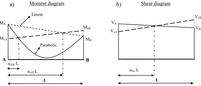
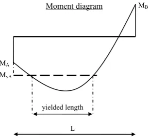
It is known that due to the presence of uniform distributed loading, the moment diagram becomes parabolic, while shear force varies linearly along the beam length. Fig. 5 illustrates the determination of moment and shear inelastic zone lengths for a beam member subjected to uniform distributed loading, when end-moments (shears) have opposite signs. It is noted that the moment and shear force distributions shown in this figure do not correspond to the same loading condition of the beam member; they are grouped together herein simply because the same methodology can be applied for the determination of their corresponding inelastic zone coefficients. In Fig. 5a, it can be seen that for sagging moments the actual inelastic zone lengths may be significantly underestimated and for hogging moments they may be seriously

overestimated, when parabolic moment distribution is not taken into account.

Figure 5. Determination of inelastic end-zone lengths when end-moments (shears) have different signs: (a) flexural sub-element; (b) shear sub-element

When end-moments (shears) have different signs, inelastic zone lengths may be determined by the location of the moment (shear) distribution, where acting moment

(shear) becomes equal to the respective end-section yield moments (MyA, MyB) or

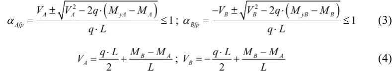
shears (VyA, VyB). Hence, the flexural yielding penetration coefficients αAfp and αBfp,

which take into consideration nonlinear moment distribution, are given by Eq. (3), where q>0 is the value of the uniform distributed loading and shear forces VA and VB

are given by Eq. (4).





2 ₂

1

A A yA A

Afp

V V q M M

q L         ;





B B yB B

Bfp

V V q M M

q L

      

 (3)

2 B A A M M q L V L     ; 2 B A B M M q L V L  

   (4)

It is noted that, when end-moments have opposite signs (Fig. 5a), Eq. (3) provides always a unique solution in the range [0, 1], when end-moments exceed the respective end-section yield moments.

ΜΒ

ΜΑ

ΜyΒ

L L

αBfp·L

αBfl·L

Linear

Parabolic ΜyΑ

αAfp·L

αAfl·L

αAs·L

VΑ

VyΑ

αBs·L

VB

VyB

a) Moment diagram b) Shear diagram

A B

It is also worth noting that, in some cases (e.g. variation of longitudinal reinforcement along R/C beam members), the yielding moments in the interior of the structural member may be different from the respective values at its end sections. This issue can be easily resolved by solving Eq. (3) for the different yield moment values and selecting the unique solution of the inelastic zone coefficient, which lies in the range of the respective yield moment.

For the calculation of the shear yielding coefficients αAs and αBs, Eq. (5) holds. It is

worth noting that the same equation provides the solution for the flexural yielding coefficients αAfl and αBfl, when linear distribution is assumed, if the shear forces are

substituted by the respective bending moments. Eqs. (3) and (5) are valid for both sagging and hogging moments as long as the absolute values of the acting moments (shears) are greater than their yielding counterparts. In these equations, the yield moments (shears) must be introduced with the same signs as the respective acting values.

A Ay As

A B

V V

V V

  

 ;

B By Bs

B A

V V

V V

  

 (5)

Fig. 6 illustrates the determination of moment and shear inelastic zone lengths for a beam member subjected to uniform distributed loading, when end-moments (shears) have the same sign; the figure presents the case, where only one member end (end A) yields.

It is noted that Fig. 6a does not represent the typical scenario for bending moments under seismic loading, but it is addressed herein since it is required for the generality of the analytical solution. Again, it can be seen that for hogging moments the actual inelastic zone lengths may be significantly overestimated when parabolic moment distribution is not taken into account.

Figure 6. Determination of inelastic end-zone lengths when end-moments (shears) have same signs: (a) flexural sub-element; (b) shear sub-element.

When end-moments (shears) have same signs, inelastic zone lengths may reach high values (Fig. 6b). Hence, it is proposed herein that they are determined by the location of the moment (shear) distribution, where acting moment (shear) meets the line connecting end-section yield moments, as shown in Fig. 6. Under this assumption, the flexural inelastic zone coefficients αAfp and αBfp are given by Eq. (6), where values

VA,eq and VB,eq are given by Eq. (7). It is noted that Eq. (6) applies only to the member

ends, where acting moments exceed the corresponding yield moments.

ΜyB

ΜΑ

ΜΒ

L

Linear

Parabolic ΜyΑ

αAfl·L

αAfp·L

a) Moment diagram b) Shear diagram

B A

VyB

VΑ

VΒ

L

VyΑ





, , 2

A eq A eq yA A

Afp

V V q M M

q L

     

 ;





2

, , 2

B eq B eq yB B

Bfp

V V q M M

q L

     

 (6)

,

yB yA A eq A

M M V V L    ; , yB yA B eq B

M M

V V

L



  ; (7)

Similarly, for the shear yielding coefficients αAs and αBs, Eq. (8) holds, which

provides also the solution for the flexural yielding coefficients αAfl and αBfl, by

substituting shear forces with the corresponding bending moments.

A yA As

A yA yB B

V V

V V V V

  

   ;

B yB Bs

B yB yA A

V V

V V V V

  

   (8)

When one acting end-moment (shear) is higher than the respective value at yield while the other is not, then Eqs. (6 to 8) provide unique solutions in the range [0, 1]. Furthermore, for the case of sagging parabolic moments and linearly distributed shear forces, if both end-moments (shears) are higher than their yield counterparts, then the entire moment (shear) diagram exceeds the line connecting the yield values of the member ends. Consequently, the entire beam member can be considered to be ‘yielded’. For these cases, following the suggestions of Reinhorn et al. (2009), it is assumed that

0.5 Af

  ; Bf 0.5;As0.5; Bs 0.5;

2 _{A B}

o A B EI EI EI EI EI     ;

2 _{A B}

o A B GA GA GA GA GA   

 (9)

For hogging parabolic moments, if both end-moments are higher than their yield values, then two cases may arise: Eq. (6) has either two or no solutions in the range [0, 1]. In the first case, the solution providing the lower value of the inelastic zone

lengths αAfp and αBfp is adopted. In the second case, the complete member is

considered as having yielded and Eq. (9) is applied.

In all cases, inelastic zone coefficients are first calculated for the current moment (shear) distribution. Then, they are compared with their previous maximum values; inelastic zone coefficients cannot be smaller than their previous maxima (Soleimani et al. 1979; Reinhorn et al. 2009). Moreover, special measures are taken to adjust flexibility distribution of members, when the sum of the two inelastic zone coefficients at the member ends exceeds unity (αA + αB>1). In such cases, the elastic

stiffness EIo (GAo) is properly modified to capture actual flexibility distribution

(Reinhorn et al. 2009).

cases where internal hinges are expected, e.g. in analysis considering the vertical component of the earthquake, it is proposed herein that the beam member is divided into a sufficient number of finite elements. In most cases this can be omitted, since these members are not the critical ones in the assessment of the structure.

Figure. 7. Development of internal inelastic zone

2.5 Flexibility coefficients

Having established the flexural and shear stiffness distributions along the beam member at each step of the analysis, the coefficients of the flexibility matrix of the flexural and shear sub-element can be derived by applying the principle of virtual work.

For the flexural flexibility coefficients, the general Equation (10) holds, where mi(x)

and mj(x) are the moment distributions due to a virtual unit end moment at end A and

B respectively, and EI(x) is the tangent flexural stiffness distribution along the beam member.

 

 

 

m x m x

f dx

EI x







For the stiffness distributions shown in Fig. 4, Eq. (10) yields the closed-form solution of Eq. (11), where the parameters co, cA, cB are defined in Table 1.





12 12

fl fl

ij o A A B B ij

o o

L L

f c c c

EI   EI 

       ; o 1

A A

EI EI

   ; o 1

B B

EI EI

   (11)

For the shear flexibility coefficients, the general Eq. (12) holds, where vi(x) and vj(x)

are the shear distributions due to a virtual unit end moment at end A and B respectively, and GA(x) is the tangent shear stiffness distribution along the beam member.

   

 

v x v x

f dx

GA x





_

It can be shown that for the stiffness distributions shown in Fig. 4, Eq. (12) yields the closed-form solution of Eq. (13), where the parameters do, dA, dB are defined in Table

1.





1 1

sh sh

ij o A A B B ij

o o

f d d d

GA L   GA L 

      

  ; 1

o A

A

GA GA

   ; o 1

B B

GA GA

   (13)

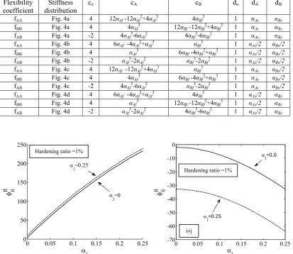
Fig. 8 illustrates the variation of the normalized flexural flexibility coefficients φflii ΜΒ

ΜΑ

L ΜyΑ

yielded length

values developed under seismic loading 0≤αi, αj≤0.25 (Filippou and Issa 1988). It is

assumed that the stiffness distribution is uniform in the inelastic zones and that the ratio of the post elastic to the elastic flexural stiffness is equal to 1%. Two limit cases are examined. In the first case, the yielding penetration coefficient of the j section is equal to zero and in the second case it is equal to 0.25. The strong dependence of the flexibility matrix coefficients from the inelastic zone coefficients is evident. This observation emphasizes the need for accurate simulation of the spread of inelasticity.

Table 1. Determination of flexural and shear flexibility matrix coefficient parameters

Flexibility coefficient

Stiffness distribution

co cA cB do dA dB

fAA Fig. 4a 4 12αΑf -12αΑf2+4αΑf3 4αΒf3 1 αΑs αBs

fBB Fig. 4a 4 4αΑf3 12αΒf -12αΒf2+4αΒf3 1 αΑs αBs

fAB Fig. 4a -2 4αΑf3-6αΑf2 4αΒf3-6αΒf2 1 αΑs αBs

fAA Fig. 4b 4 6αΑf -4αΑf2+αΑf3 αΒf3 1 αΑs/2 αBs/2

fBB Fig. 4b 4 αΑf3 6αΒf -4αΒf2+αΒf3 1 αΑs/2 αBs/2

fAB Fig. 4b -2 αΑf3-2αΑf2 αΒf3-2αΒf2 1 αΑs/2 αBs/2

fAA Fig. 4c 4 12αΑf -12αΑf2+4αΑf3 αΒf3 1 αΑs αBs/2

fBB Fig. 4c 4 4αΑf3 6αΒf -4αΒf2+αΒf3 1 αΑs αBs/2

fAB Fig. 4c -2 4αΑf3-6αΑf2 αΒf3-2αΒf2 1 αΑs αBs/2

fAA Fig. 4d 4 6αΑf -4αΑf2+αΑf3 4αΒf3 1 αΑs/2 αBs

fBB Fig. 4d 4 αΑf3 12αΒf -12αΒf2+4αΒf3 1 αΑs/2 αBs

fAB Fig. 4d -2 αΑf3-2αΑf2 4αΒf3-6αΒf2 1 αΑs/2 αBs

0 0.05 0.1 0.15 0.2 0.25

-70 -60 -50 -40 -30 -20 -10 0

_i



fl ij



j=0.0



j=0.25

Figure 8. Variation of the normalized flexural flexibility matrix coefficients with the yielding penetration coefficients for hardening ratio 1% and uniform stiffness distribution in the inelastic zones.

3. Numerical model validation

In this section, the proposed numerical model is validated against the analytical solutions provided in Anagnostopoulos (1981) for prismatic beam members whose

cross section response can be adequately represented by a bilinear M-φ curve (with

hardening ratio r) in monotonic loading (Fig. 2). Shear flexibility is ignored in both the numerical and the analytical solutions.

0 0.05 0.1 0.15 0.2 0.25

0 50 100 150 200 250

_i



fl ii

 j=0.25

_j=0

Hardening ratio =1%

i≠j

In the analytical study by Anagnostopoulos (1981), beam loading consists of two end

rotation increments (Fig. 1) ΔθΑ and ΔθΒ (differences between maximum and yield

rotations) with ratio ΔθΑ/ΔθΒ=n. It is also assumed that before these rotations are

applied, the member is bent by two end moments MA and MB where MA=c·My and

MB=My. My is the common yield moment of both end sections, assumed the same in

positive and negative bending. The imposed end rotations are assumed to act with or without the presence of a uniform distributed loading q, superimposing a bending moment MG=q·L2/8 in the middle of the beam member.

The analytical solutions provide the post-yield secant stiffness ratios Si (i=A,B) as a

function of the imposed rotation ductility demands μθi for both member ends. The

post-yield secant stiffness ratios are defined as

i

i i

i

S

K 

   _ 

 

 (14)

where ΔΜi is the moment increment at end i (difference between maximum and yield

moment) and Ki is the elastic stiffness, which is equal to 6EIo/L for n=1

(antisymmetric bending).

In the following, the analytical solutions will be compared with the results of the proposed numerical model for the following conditions: n=1, c=1, r=0.05. Regarding

beam distributed loading q, two separate cases are examined: MG=0 (i.e. q=0) and

MG=0.5My.

To simulate the above conditions, a symmetric beam member with properties EIo=104kNm2, My=103kNm, φy=10-1m-1, L=10m, r=0.05 and q=0 or q=40kN/m, was

subjected to pushover analysis using the proposed finite element model.

Fig. 9 compares the predicted Si values as a function of the imposed μθi by the

proposed numerical model and the analytical solutions by Anagnostopoulos (1981). Circles represent some discrete results of the analytical solutions (obtained by the use of special software for digitizing graphical data) and the continuous lines the predictions of the proposed numerical model. It is seen that the matching between the two solutions is excellent.

0.0 0.1 0.2 0.3 0.4 0.5

1 4 7 10

Si

μ_θi

MG=0.5My& Mi<0

MG=0.5My& Mi>0

M_G=0

Analytical solution Proposed model

It is important to note that post-yield secant stiffness decreases faster with μθi for

sagging moments (Mi>0) than for hogging moments, when distributed beam loading

q is present. This occurs because the length of the inelastic zone is greater for the

member end with the sagging moment for the same value of ΔΜi. The solution

without distributed loading lies between the solutions for sagging and hogging moments, when distributed loading is applied. All curves tend to Si=1 for μθi=1.

4. Numerical model implementation

The proposed member-type model is implemented in a computer program (IDARC2D) for the nonlinear dynamic analysis of R/C structures (Reinhorn et al. 2009). It is then used for the inelastic static and dynamic analyses of plane frame structures with beam members dominated either by flexure or shear. In these analyses, the column members are modelled by the existing column element of IDARC2D, which accounts for axial flexibility and it is accurate for linear moment diagrams. In addition to the above, parametric analyses are conducted in order to investigate the influence of beam gravity loading on inelastic seismic response of frame structures.

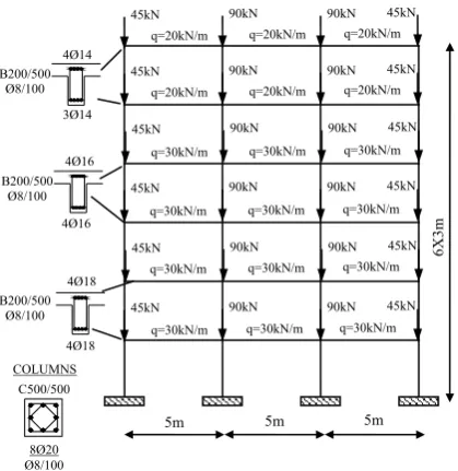
4.1 R/C Frame structure with flexure dominated beam members

The six-storey frame examined herein is part of an R/C building designed according to EC8 for a ground acceleration of 0.36g. The materials used in the structure are C25/30 (characteristic cylinder strength of 25 MPa) concrete and B500c steel (characteristic yield strength of 500 MPa). The total dead and live loads on the floor slabs are assumed to be 6.5kN/m2 and 2.0kN/m2, respectively. In addition, infill walls represented by linear distributed loads 10kN/m are present on the first four storeys of the frame. Frame layout, vertical loads for the seismic combination and cross-section details are presented in Fig. 10. It is noted that due to the application of capacity design principles, only flexural yielding is expected to be developed for the beam members of the frame.

To investigate the importance of distributed loading, three different models are set up for the inelastic seismic analysis of this frame. Model 1 assumes a constant hinge length equal to 0.08Ls, where Ls is the member shear span; Ls is taken equal to L/2 for

Figure 10. R/C frame layout with flexure-dominated beam members

Fig. 11 illustrates pushover curves derived using the three analytical models for the examined frame. It can be seen that the three models yield insignificant differences in terms of lateral stiffness. However, noticeable variations are observed for the maximum displacement capacities assumed to coincide with the first exceedance of curvature capacity in a base column. Top displacement capacity over building height is predicted as 3.7%, 4.1% and 4.6% by analytical models 1, 2 and 3, respectively.

0 0.05 0.1 0.15 0.2

0 1 2 3 4 5

Vbas

e

/ W

Δ_top/ H (%)

Model 1 Model 2 Model 3

Figure 11. Pushover curves derived using the three different analytical models

Fig. 12a presents column maximum curvature ductility (μφ) demands at 3% top

drift, which can be considered as a conventional limit for lateral failure (Kappos 1991). These demands are almost identical except for the base columns, where model 1 slightly overestimates μφdemand.

In addition, Fig. 12b shows variation of beam maximum μφ demands, also at 3%

top drift. In contrast with column demands, predicted beam μφ demands differ

substantially. Higher μφdemands are calculated by the proposed analytical model of

the present study. Hence, ignoring beam distributed loading may drive the analysis to serious underestimation of end-section curvature demands. The common assumption

of linear moment distribution underestimates μ demands at the beam ends subjected

q=20kN/m

5m 5m 5m

6X

3m

C500/500

8Ø20 Ø8/100 COLUMNS B200/500

Ø8/100

4Ø18 4Ø18 4Ø14

3Ø14 B200/500

Ø8/100

B200/500 Ø8/100

4Ø16 4Ø16

q=30kN/m q=30kN/m q=30kN/m q=30kN/m q=30kN/m q=30kN/m

q=30kN/m q=30kN/m q=30kN/m q=30kN/m q=30kN/m q=30kN/m q=20kN/m q=20kN/m

q=20kN/m q=20kN/m q=20kN/m

45kN 90kN 90kN 45kN

45kN 90kN 90kN 45kN

45kN 90kN 90kN 45kN

45kN 90kN 90kN 45kN

45kN 90kN 90kN 45kN

to hogging moments. At these ends, inelastic zone lengths are over-predicted (Fig. 5) and similar rotations are calculated for lower μφ demands.

Figure 12. Maximum curvature ductility demands at 3% top drift: (a) columns; (b) beams

This can be seen also in Fig. 13, which illustrates the expansion of flexural inelastic zone coefficient in relation to end section curvature demand for the first story middle beam. Results up to 3% top drift are presented for all applied analytical models. Fig. 13a refers to the beam end subjected to sagging moments and Fig. 13b to the member end developing hogging moments. It is clear that the assumption of linear moment distribution overestimates inelastic zone coefficient and underestimates curvature demand for hogging moments; the opposites hold for sagging moments.

Figure 13. Variation of inelastic zone coefficients with end-section curvature demand for the middle 1st _{storey beam: (a) sagging; (b) hogging moments}

In the following, the response of the R/C frame of Fig. 10 under the near-field ground motion recorded at JMA Kobe Observatory (NS component) with PGA=0.59g is investigated. In particular, Fig. 14a illustrates top displacement history responses derived by the three analytical models. Differences are small, albeit not negligible. Deviations become more significant, when comparing maximum story drifts, shown in Fig. 14b. Model 1 overestimates drift at the lower storeys and underestimates them at the high storeys. Models 2 and 3 predict similar drifts at the first story level, but yield significant deviations at the top two storeys.

0 1 2 3 4 5 6

0 5 10 15 20

St

or

ey

μ_φ

Model 1 Model 2 Model 3

0 1 2 3 4 5 6

0 5 10 15 20 25 30 35

St

ore

y

μ_φ

Model 1 Model 2 Model 3

0.00 0.02 0.04 0.06 0.08 0.10

-0.05 0.00 0.05 0.10 0.15 0.20

Inelastic zone

coef

ficient

Curvature (rad/m)

Model 1 Model 2 Model 3

0.00 0.02 0.04 0.06 0.08 0.10

-0.30 -0.20 -0.10 0.00

In

ela

stic zone

coef

fi

ci

ent

Curvature (rad/m) Model 1

Model 2 Model 3

a) b)

Figure 14. R/C frame responses under JMA Kobe NS component ground motion: (a) top displacement; (b) maximum story drifts

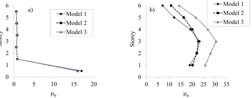
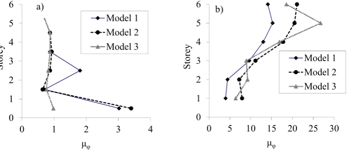
Finally, Fig. 15 shows maximum μφ demands derived using the three analytical

models for the specific ground motion. It is clear that significant discrepancies are observed for the three analytical models. This points to the need of properly modelling the effect of distributed loading on gradual spreading of inelastic flexural deformations, in the inelastic response history analysis of frame structures.

Figure 15. Maximum μφ demand predictions under JMA Kobe NS component ground motion:

(a) columns; (b) beams

4.2 Portal frame with shear-dominated beam member

The following example, taken from the IDARC2D report (Reinhorn et al. 2009), is a theoretical example intended to demonstrate the program’s capability for modelling frame structures with beams yielding in shear. It is a portal frame composed of two columns with similar sectional characteristics and one beam (Fig. 16).

For the two columns, shear deformations can be neglected without loss of accuracy. However, this is not the case for the connecting beam member, which is characterized

by low initial shear stiffness GA and limited shear yield capacity Vy. Furthermore,

unlike the example included in the IDARC report, the beam member of the frame examined herein is subjected to a uniformly distributed vertical loading q=2kN/m. Hence, the total weight of the frame becomes 48.4kN.

Pushover analysis of this frame is conducted up to the point where curvature demand

reaches column curvature capacity φ . The beam member does not yield in flexure.

-400 -200 0 200 400

0 5 10 15

Di

spl

ace

m

en

t (mm

)

Time (sec)

Model 1 Model 2 Model 3

0 1 2 3 4 5 6

0 1 2 3 4 5

Stor

ey

Drift (%)

Model 1 Model 2 Model 3

0 1 2 3 4 5 6

0 1 2 3 4

St

or

ey

μφ

Model 1 Model 2 Model 3

0 1 2 3 4 5 6

0 5 10 15 20 25 30

Storey

μ_φ

Model 1 Model 2 Model 3

a) b)

Nevertheless, the beam does yield in shear at its right end. The same is not observed for the left and middle sections of the beam, which remain in the elastic range. The reason for this behaviour becomes evident in Fig. 17a. In this figure, it can be seen that, due to the existence of the distributed loading, shear forces vary along the beam member. In particular, as analysis progresses, shear forces at the three different sections increase in a proportional manner. The constant differences between these lines represent the influence of the distributed loading. In the same figure, it is clear that right section shear force exceeds yield shear at analysis step 530. At the same step, the value of the right shear yielding penetration coefficient (Fig. 17b) begins to increase from zero to 0.46 at the end of the analysis. The latter value agrees well with the middle line of Fig. 17a, which shows that the middle beam section is very close to yielding in shear.

Fig. 18 illustrates pushover curves obtained by three different analytical models for the frame. Model 1 neglects beam shear flexibility. Model 2 accounts for beam shear flexibility. However, distributed loading effect is ignored and shear force is assumed to be constant along the beam member and equal to the actual shear force at the middle section (uniform distributed loading yields zero shear in the middle of the beam). Finally, model 3 is the one proposed in this study.

It is evident that ignoring shear flexibility leads the pushover analysis to serious overestimation of frame lateral stiffness and strength and significant underestimation of displacement capacity. Furthermore, comparing models 2 and 3, it can be seen that the proposed model deviates from model 2, when yielding of the beam right end section occurs. Neglecting gradual spread of inelastic shear deformations by model 2, drives the analysis to considerable overestimation of lateral stiffness and strength and under-prediction of displacement capacity.

Figure 16. Frame with shear-dominated beam member

50m

m

1500m

m

2000mm Rigid arms

EI=262kNm2

My=17kNm

r=1%

φu=1.0rad/m

EI=262kNm2 _{, M}

y=17kNm, r=1%

GA=500kN, Vy=7kN, r=1%

q=2kN/m

EI=262kNm2

My=17kNm

r=1%

φu=1.0rad/m

Figure 17. Beam member response: (a) progression of shear forces at different sections; (b) gradual increase of the shear-yielding penetration coefficient

0 0.2 0.4 0.6 0.8 1 1.2

0 2 4 6 8 10

Vba

se

/ W

Drift (%) Model 1 Model 2 Model 3

Figure 18. Pushover analysis curves derived by three different analytical models

5. Conclusions

A new gradual spread inelasticity finite element was developed for seismic analysis of beam members with uniform distributed loading. Unlike common inelastic beam elements, the proposed model is able to account consistently for the effect of distributed loading on the variation of flexural and shear stiffness along the beam members throughout their inelastic response. The finite element is accurate for beam members subjected typically to uniaxial bending without axial loading, as well as computationally efficient since it requires monitoring hysteretic response only at the member end sections.

The numerical model was implemented in a general inelastic dynamic analysis finite element code and was used for the analysis of R/C plane frames with beam members dominated either by flexure or shear. It was shown that distributed beam loading effect should be properly and accurately taken into account in the inelastic static and dynamic analysis of frame structures.

0 0.1 0.2 0.3 0.4 0.5

0 500 1000

In

ela

stic

zo

ne

c

oef

ficien

t

Analysis step -4

-2 0 2 4 6 8 10

0 500 1000

Sh

ea

r (k

N)

Analysis step

Left end Middle Right end

Yielding shear

References

Anagnostopoulos, S. (1981), "Inelastic beams for seismic analysis of structures",

Journal of Structural Engineering, 107(7), 1297-1311.

Addessi, D. and Ciampi, V. (2007), "A regularized force-based beam element with a

damage-plastic section constitutive law", International Journal of Numerical

Methods in Engineering, 70(5), 610-629.

Beyer, K., Dazio, A. and Priestley, M.J.N. (2011), "Shear deformations of slender R/C walls under seismic loading", ACI Structural Journal, 108(2), 167-177.

Ceresa, P., Petrini, L. and Pinho, R. (2007), "Flexure-shear fibre beam-column elements for modeling frame structures under seismic loading. State of the art",

Journal of Earthquake Engineering, 11(1), 46-88.

Clough, R. and Johnston, S. (1966), "Effect of stiffness degradation on earthquake

ductility requirements", Transactions of Japan Earthquake Engineering

Symposium, Tokyo, 195-198.

Filippou, F. and Issa, A. (1988), Nonlinear analysis of R/C frames under cyclic load

reversals, Report EERC-88/12, Univ. of California Berkeley.

Giberson, M. F. (1967), The response of nonlinear multi-story structures subjected to

earthquake excitation, Ph.D. thesis, Cal. Tech., Pasadena, California.

Kappos, A.J. (1991), "Analytical Prediction of the Collapse Earthquake for R/C

Buildings: Suggested Methodology", Earthquake Engineering & Structural

Dynamics, 20 (2), 167-176.

Kyakula, M. and Wilkinson, S. (2004), "An improved spread plasticity model for inelastic analysis of R/C frames subjected to seismic loading", Proc. of the 13th World Conf. Earthquake Engineering, Vancouver, B.C., Canada.

Lee, C. L. and Filippou, F. (2009), "Efficient beam-column element with variable inelastic end zones", Journal of Structural Engineering, 135(11), 1310-1319.

Lehman, D. and Moehle, J.P. (1998), Seismic Performance of Well Confined Concrete

Bridge Columns, PEER Report 1998/01, Univ. of California, Berkeley.

Mergos, P.E., and Kappos, A.J. (2008), "A distributed shear and flexural flexibility model with shear-flexure interaction for R/C members subjected to seismic

loading", Journal of Earthquake Engineering and Structural Dynamics, 37(12),

1349-1370.

Mergos, P.E., and Kappos, A.J. (2009), "Modelling gradual spread of inelastic flexural, shear and bond-slip deformations and their interaction in plastic hinge

regions of R/C members", Proc. of 2nd COMPDYN Conference, Rhodes, Greece.

Mergos, P.E. and Kappos, A.J. (2012) "A gradual spread inelasticity model for R/C

beam-columns, accounting for flexure, shear and anchorage slip", Engineering

Structures, 44, 94-106.

Meyer, C., Roufaiel, S.L. and Arzoumanidis, S.G. (1983), "Analysis of damaged

concrete frames for cyclic loads", Journal of Earthquake Engineering and

Structural Dynamics, 11(2), 207-222.

Neuenhofer, A. and Filippou, F.C. (1997), "Evaluation of nonlinear frame finite-element models", Journal of Structural Engineering, 123(7), 958-966.

Reinhorn, A.M., Roh, H., Sivaselvan, M., Kunnath, S.K., Valles, R.E., Madan, E., Li,

C., Robo, L., and Park, Y.J. (2009), IDARC2D version 7.0: A program for the

Roh, H., Reinhorn, A.M. and Lee, J.S. (2012), "Power spread plasticity model for inelastic analysis of reinforced concrete structures", Engineering Structures, 39, 148-161.

Sivaselvan, M.V. and Reinhorn, A.M. (2000), "Hysteretic models for deteriorating inelastic structures", Journal of Engineering Mechanics, 126(6), 633-640.

Soleimani, D., Popov, E.P. and Bertero, V.V. (1979), "Nonlinear beam model for R/C frame analysis", Proc. of 7th Conf. on Electronic Computation, Struct. Div. ASCE, Washington, 483-509.

Spacone, E., Filippou, F.C. and Taucer, F.F. (1996), "Fiber beam-column model for

nonlinear analysis of R/C structures: Formulation", Journal of Earthquake