MLPG_R method for modelling 2D flows of two immiscible fluids

City, University of London Institutional Repository

Citation:

10.1002/fld.4353

This is the accepted version of the paper.

This version of the publication may differ from the final published

version.

Permanent repository link:

Link to published version:

Copyright and reuse: City Research Online aims to make research

outputs of City, University of London available to a wider audience.

Copyright and Moral Rights remain with the author(s) and/or copyright

holders. URLs from City Research Online may be freely distributed and

linked to.

City Research Online: http://openaccess.city.ac.uk/ [email protected]

This article has been accepted for publication and undergone full peer review but has not been through the copyediting, typesetting, pagination and proofreading process which may lead to differences between this version and the Version of Record. Please cite this article as

MLPG_R method for modelling 2D flows of two immiscible fluids

Yan Zhou, Q.W. Ma* and S. Yan

School of Mathematics, Computer Science and Engineering, City University London *Corresponding author email: [email protected]

Abstract

This is a first attempt to develop the Meshless Local Petrov-Galerkin method with Rankine source solution (MLPG_R method) to simulate multiphase flows. In this paper, we do not only further develop the MLPG_R method to model two-phase flows but also propose two new techniques to tackle the associated challenges. The first technique is to form an equation for pressure on the explicitly identified interface between different phases by considering the continuity of the pressure and the discontinuity of the pressure gradient (i.e., the ratio of pressure gradient to fluid density), the latter reflecting the fact that the normal velocity is continuous across the interface. The second technique is about solving the algebraic equation for pressure, which gives reasonable solution not only for the cases with low density ratio but also for the cases with very high density ratio, such as more than 1000. The numerical tests show that the results of the newly developed two-phase MLPG_R method agree well with analytical solutions and experimental data in the cases studied. The numerical results also demonstrate that the newly developed method has a second-order convergent rate in the cases for sloshing motion with small amplitudes.

Key Words: Meshless method, multiphase flow, high density ratio, MLPG_R method, sloshing.

1.

Introduction

Multiphase flows are found in both natural environment and industry applications consisting of different fluid phases immiscible to each other. Examples include the sloshing motion in the LNG (Liquefied Natural Gas) tanks, internal waves in ocean and water impact on structures in marine engineering. In these cases, the density ratio can approach 1 for stratified fluid flows and can reach more than 1000 for the water-air flows. In addition, surface tension effects can be ignored and the viscous effects play relatively less important role compared to the inertial effects in these cases.

solve the two-phase flow equations can be either mesh-based or meshless. There is a large volume of publications related to the mesh-based methods. As it is not our focus to review them in this paper, only brief discussions are given here. In the mesh-based methods, different fluid phases are often treated as ‘one-fluid’ and the changing of fluid properties across the interface, such as density and viscosity field, is taken into account by a marker function. Several approaches have been developed such as volume of fluid (VOF) [1, 2], level-set [3]–[5] and coupled VOF and level-set [6]–[9] methods. They are usually implemented together with fixed grids or meshes. In this kind of methods, the density and viscosity are determined by the marker function through the interface over several cells, that is, the marker function, together with all other physical quantities, are smoothed within a layer. In addition, these methods need to deal with the convection which can cause artificial numerical diffusion, and need to find the solution for the extra marker function, which requires extra computational time.

There are also a number of attempts to adopt meshless methods, including Smooth Particle Hydrodynamics (SPH) and Moving Particle Semi-implicit (MPS) methods. Unlike mesh-based methods, the interface in meshless methods is traced by Lagrange moving particles without use of any marker functions, and the convection terms do not need to be dealt with. It is now well known that there are largely two kinds of formulations in the meshless methods. One is based on the projection scheme, in which Poisson’s equation needs to be solved. The other is based on the equation of state to determine the relationship between the pressure and density. The latter does not need to solve the boundary value problem but relies on the use of very small time steps, perhaps 10 times smaller than the steps to be used by the former [10]. Multiphase MPS was first introduced by [11] for solid-liquid flow. Recently a weakly compressible MPS [12] was developed which introduced the equation of state to original MPS method. In [12] a smoothing scheme based on the spatial averaging of density and a harmonic mean for viscosity on interfaces was adopted. However, as pointed out by [13], the zero order smoothing may downgrade the accuracy in capturing the sharp variation of density at the interface and subsequently lead to unphysical dispersions of particles near the interface. Khayyer, et al. [13] considered two phases as one fluid and adopted the projection scheme. They also proposed a first order density smoothing based on Taylor series expansion. Despite that the density was still spatially averaged, this higher order smoothing technique significantly enhanced the accuracy of density reconstruction near the interface. Together with improved gradient estimation, the multiphase MPS in the cited paper is able to model flows with a high density ratio of 1000.

of cases with high density ratios. However, additional techniques such as density re-initialization based on first order moving least square (MLS) method, artificial viscosity, velocity correction and cohesion force were required to prevent pressure oscillation and unphysical particle inter-penetration at the interface. To overcome the problems, Hu and Adams [17] proposed an evolution equation for the particle density and a particle-averaged spatial derivative by introducing a particle approximation function involving the volume of neighbouring particles rather than the density as in other SPH modelling. Adoption of an artificial repulsive force between two fluids is an alternative compensation to avoid interface fragmentation and to achieve stable simulations for density ratios as high as 1000 [18,20]. Hu and Adams [21,22] developed a multiphase ISPH model by using a smoothing function which naturally handled density discontinuity across the interface. The interface conditions of continuous pressure and specific pressure gradient (hereafter specific pressure gradient referring to the ratio of pressure gradient to fluid density) were implemented by introducing an inter-particle-averaged directional derivative when solving Poisson’s equation. The implementation assumes that the interface is at the middle of each pair of neighbouring particles with different densities and the normal of the interface is in the direction of the connection line between that pair of particles. As such approximation required many pairs of particles in the range of an influencing domain of a concerned point, the interface so determined was actually a layer with a thickness in an order of the influencing domain size, about double distance of two particles. Shao [23] presented both coupled and decoupled ISPH two-phase flow models. The coupled model actually considered the two phases as one fluid and estimated the density by using standard SPH approach smearing it across the interface and solved the one pressure Poisson’s equation for the whole domain, while the decoupled model considered the two fluids separately but were coupled at interface, in which the pressure continuity condition was explicitly imposed without considering the specific pressure gradient. They found that the decoupled model performed better than the coupled model for the flow with a higher density ratio of 1.3. A hybrid model combining the ISPH for water phase with CSPH for air phase was recently proposed in [24], which achieved successful simulation of cases with a high density ratio (e.g., dam breaking) with the predicted pressure agreeing well with experimental data. At the interface, pressure and velocity were provided for each other phase. When they solved Poisson’s equation for water, the pressure at the interface is estimated by using the pressure from the previous time step at all particles of both phases.

In the projection-based modelling, a major task is to solve Poisson’s equation. In most publications related to MPS and ISPH so far, the second derivatives are directly approximated by using various schemes, see for example, [25] and [26]. According to the investigations by [27] and [25], the convergent rate of methods based on this approach may be low (much less than 2nd order) when the disorderliness of particle distribution is high. The disorderliness may be reduced by introducing the Fickian shifting algorithm [28] to move particles from regions of high concentration to regions of low concentration, leading to better results. More details can be found in the recent review paper by Ma, et al. [29].

The meshless local Petrov-Galerkin method based on Rankine source (MLPG_R method) proposed by [30] offers an alternative. Similar to the ISPH and MPS methods, the MLPG_R method is also a meshless particle method based on the projection scheme. However, the MLPG_R method distinguishes from the ISPH and MPS methods in the following two aspects at least. Firstly, in this method, Poisson’s equation is transferred into a weak form that does not contain any derivatives of the pressure or unknown quantities to be solved and therefore the numerical approximation of the first and second derivatives of the pressure or unknown quantities is completely removed when solving Poisson’s equation. This is compared with the approach adopted in the ISPH and MPS methods that seeks to directly approximate or discretise the second derivatives involved in the Poisson’s equation as indicated above. Secondly, the MLPG_R method is equipped with an efficient semi-analytical integration method [30] to evaluate the integrals involved in the weak form, which is not involved in the ISPH and MPS methods. Zheng, et al. [27] demonstrated that the method based on the approach of the MLPG_R can achieve 2nd order convergent rate by studying the sloshing waves with small amplitudes. The robustness of the MLPG_R method have also been demonstrated by applying it to solve a wide range of wave-structure interaction problems, such as violent waves [31] and their interactions with both rigid structures [31] and elastic structures [32].

Figure 1: Particle representation of the two-phase flow with phase ( ) and ( ) being separated by interface particles ( )( ). Also shown are the integral domain and the support domain with a diameter of .

2.

Formulation of two-phase MLPG_R method

As illustrated in Figure 1, the problem discussed in this paper is about flows containing two immiscible and incompressible phases of and . These two phases are separated by a continuous interface consisting of interface particles. The applications of our method are mainly to marine engineering, where the waves formed on the interface are assumed to be quite long and associated Reynolds number is quite large. As a result, the surface tension may not be considered and the viscous effects are relatively weak compared to inertial effects as indicated by Lind, et al. [24].

2.1.

Governing equations

The motion of inner particles (i.e. particles located neither at the rigid boundaries nor interfaces) is governed by the incompressible Navier-Stokes equations without considering surface tension and the continuity equation which can be written as

(1)

(2)

where is the gravitational acceleration, is the fluid velocity vector, is the pressure, is the fluid density and is the fluid viscosity. The subscript presents the phase that particles belong to, for which . The motion of particles in either phase is driven by gravity, pressure gradient and viscous force as in other Lagrangian multiphase approaches (e.g., [12], [19]).

At a rigid wall boundary, the normal component of the fluid velocity equals to that of the boundary velocity

(3)

Considering the normal components of both sides of Eq. (1) and substituting Eq. (3), the pressure satisfies the following condition on the rigid boundaries as in single phase MLPG_R method [31]:

(4)

where and are the velocity and the acceleration of the rigid boundary respectively, assumed to be specified in this paper.

(5)

As Fedkiw, et al. [33] pointed out that the tangential velocity on the interface may be continuous or discontinuous depending on whether the no-slip condition is imposed. They particularly indicated that the tangential velocity should be considered to be discontinuous for a shear wave. This paper mainly concerns multiphase flow in marine engineering, where the dynamic viscosity of fluids, such as water and air, is very small ( ) and plays a less important role as discussed by [20] and [34]. In addition, the results for wind-wave interaction in [35] and for water-air sloshing in [36] demonstrate that the tangential velocity near interface can change from one direction to another in a thin layer, typical shear flow phenomenon. Based on these facts, the tangential velocity is not constrained to be continuous, i.e., ‘slip’ condition may be applied on the interface like on a rigid boundary. The stress condition at the interface can be simplified to be pressure continuity by neglecting the viscous stress and interface tension as in [34] and [24] and many other papers, i.e.

(6)

The model is numerically solved by a time marching procedure consisting of prediction and correction steps. The details of the procedure can be found in [31] for single phase flow and here only a brief summary will be given below. Suppose that variables of pressure, velocity and location of each particle are known at the n-th time step ( ) and those will be updated at n+1-th time step according to the following prediction and correction steps.

(a) Prediction step

The intermediate velocity ( ) and position ( ) are calculated by

(7)

(8)

(b) Correction step

Pressure is solved using the following Poisson’s equation

(9)

(10)

The velocity and position of n+1-th step are updated by

(11)

(12)

3.

Numerical formulation of pressure equation

The numerical formulation of pressure equation will be different for inner, wall boundary and interface particles. At the inner and wall boundary particles, the pressure is treated using the same technique as in the single phase MLPG_R method while the pressure at the interface particles is determined by enforcing the interface conditions discussed above.

3.1. Inner particles

For inner particles, pressure is solved in a weak form (Eq. (13)) of the Poisson’s equation (Eq. (9)). The details of the formulation are similar to those in [30] and only the final expression is presented here:

(13)

where is the unit vector normal to integration sub-domain and pointing outside,

is the solution of the Rankine source in an unbounded 2D domain with and

being the distance away from the centre of the sub-domain and the radius of the integration domain, respectively. Without the need of approximating the second order derivative of the unknown pressure as in MPS [37] and ISPH [10] methods, this weak formulation is discretised by interpolating unknown pressure using the moving least square (MLS) method, and numerically integrating the right hand side of Eq. (13) by a semi -analytical technique [30]. This feature potentially improves the accuracy in solving pressure equation and detailed comparisons may be found in [27].

3.2. Interface particles

Two conditions should be applied at the particles on the fluid-fluid interface, i.e., the continuity of pressure and the velocity when solving Poisson’s equation for pressure. As discussed in the Introduction section, there are largely three types of ways to implement the conditions in meshless methods in literature: (1) treating multiphase as one fluid without explicitly imposing interface conditions, e.g., [12], [13] and [23]; (2) explicitly enforcing the continuity of pressure (not pressure gradient), e.g., [23]; (3) explicitly enforcing the continuity of pressure and specific pressure gradient, e.g.[21], [22].

In this paper, the two conditions will be imposed explicitly and instantaneously when solving Poisson’s equation for pressure. For this purpose, the normal velocity continuity should be equivalently expressed in terms of pressure and Eq. (1) is first used to give

Use of Eq. (5) yields

Following the approach in [38] and [18], the viscous term on the interface is approximated by the average one, , and so , which gives

(14)

In addition, the fact that the pressure is continuous across the interface (i.e. Eq. (6)) implies that the tangential derivative of the pressure at the interface is also continuous, i.e.,

(15)

where denotes the tangential direction of the interface.

Combining Eq. (14) and (15), the jump of at the interface can be expressed as

(16)

where and are the unit vector in normal and tangential direction respectively. For convenience, the term of , i.e., the ratio of pressure gradient to fluid density, will be named as specific pressure gradient in this paper. Eq. (16) is a new formulation being consistent with the assumption that the tangential velocity is not necessarily continuous, and is also the main difference from [22] in which the specific pressure gradient is assumed to be continuous. It can be seen that for small density ratio of two-phase fluids or slow variation of pressure on the interface, the right hand side of Eq. (16) is near zero; on the other hand, the jump of can be significant for flows with high density ratio or significant pressure variation.

To implement the condition given by Eq. (6) and Eq. (16) in the two-phase MLPG_R method, the pressure near the interface denoted by is firstly expanded into a Taylor series separately within each phase:

(17)

(18)

Utilizing Eq. (6) and (16), Eq. (17) and (18) can be written to

(20)

where ,

and

denote the continuous quantities at the interface.

Secondly, discretizing Eqs. (19) and (20) in the support domain within each phase yields

(21) (22)

where the shape function is obtained by the moving least square (MLS) algorithm in a support domain containing both phases [30], and are total particle numbers within the support domain in phase and phase respectively.

Thirdly, adding up Eqs. (21) and (22) gives

(23)

The first two terms of the right hand side (RHS) of Eq. (23) could approach zero when sufficient particles are involved. Even though the discretisation of the last term is taken only within one phase (partial support domain), can also become close to

distribution related to the central particle. However, to consider general particle distributions, RHS of Eq. (23) will be retained and is abbreviated to . Rearranging Eq. (23) yields

(24)

Eq. (24) provides a simple and explicit pressure expression on the interface which is obtained by imposing the two conditions of Eq. (6) and Eq. (16). If we would impose the boundary condition ensuring only pressure continuity at the interface [23], the expression of Eq. (24) would be replaced by the following equation

(25)

where the subscript of represents the interface condition of pressure continuity. It can be seen that Eq. (24) could be simplified to Eq. (25) only if , (i.e. the two phases have similar densities) and which can normally be satisfied when the number of particles is sufficiently large. Therefore, it can be deduced that applying the pressure continuity alone without Eq. (16) is possible only for fluids with low density ratios.

To implement the interface condition, the interface particles need to be explicitly identified especially for the case with large deformations or breakings. The technique based on absolute density gradient developed in [39] is adopted here with the criterion of for interface particles. If the ratio is less than 0.3, the particles are justified as inner particles while those with the ratio larger than 1.5 are judged as isolated particles. In the cited paper [39], the values near the lower boundary ranging from 0.2 to 0.4 have been tested, which showed that the results are correct and not sensitive to the selection between 0.2-0.4 for the lower boundary. The tests have also been carried out for different values near the upper boundary, i.e., from 1.4 to 1.6. Again, almost all the particles can be correctly identified no matter which value between 1.4–1.6 is selected. The parameters are calculated by

, , where and are density derivatives in horizontal and vertical

directions respectively, and is the initial particle distance. More details of the technique for identifying the interface particles can be found in [39].

4.

Numerical approaches for solving pressure equation

4.1. Algorithms

The final pressure equation can be written as by combining the discretised version of Eq. (13) and Eq. (24). Specifically, it is expressed by

where and denotes the terms for the interface particles. It is noted that the elements on the up-right and the lower-left corners are zero due to the fact that Eq. (13) is not applied across the interface. is a unit matrix. and represent terms corresponding to particles within each phase. According to the discretisation of Eq. (13) and (4) as detailed in [30] and [31], their elements can be expressed by

For inner particles

For solid particles

For inner particles

For solid particles

where , and denote a particle concerned and its neighbouring particles in the support domain, respectively. The elements of and are also given by the above expressions and reflect the influence of the interface particles on inner particles through Eq. (13).

It is noted that the matrix and reflect the influence of inner particles on interface particles through Eq. (24). For this reason, generally (and ). The elements within these two matrix could be expressed as

and, and

In order to solve Eq. (26), two possible approaches would be considered. One approach is that the pressure is found by solving Eq. (26) as one set of equations, similar to the approach adopted by [22] and [13]. This is named as Integrated-1 approach in this paper for convenience. The other approach is that Eq. (26) is split into two sets of equations as below,

(27)

(28)

Within each time step, iterations may be performed, starting with . After each iteration, will be re-evaluated using the updated pressure. This approach is named as Coupled-2 approach.

4.2. Performance of Integrated-1 and Coupled-2 approaches

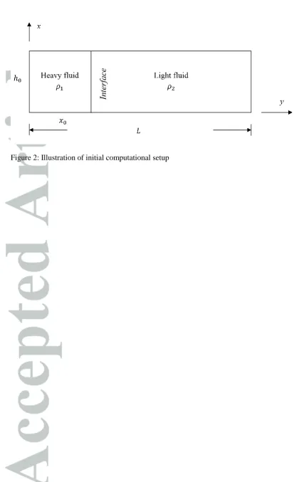
Comparisons between the Integrated-1 and Coupled-2 approaches will be made in terms of accuracy and CPU time. For the Coupled-2 approach, the effects of iterations between Eq. (27) and Eq. (28) within each time step will be first tested for different time steps. The case considered for this purpose is a gravity current formed by suddenly removing the partition between two static fluids, so that the heavier fluid flows into the lighter fluid under the effect of gravity. Figure 2 shows a schematic setup.

Figure 2: Illustration of initial computational setup

The parameters are set as , and . The density ratio

can be specified to different values. The iteration in the Coupled-2 approach is firstly tested, for which 1.01. The numbers of particles used along the depth and length are 40 and 320, respectively, thus the initial distance between particles is 0.025m. Within each time step, the error between the results at two successive iterations is calculated by

_{, where N is the total number of particles, and the criterion for}

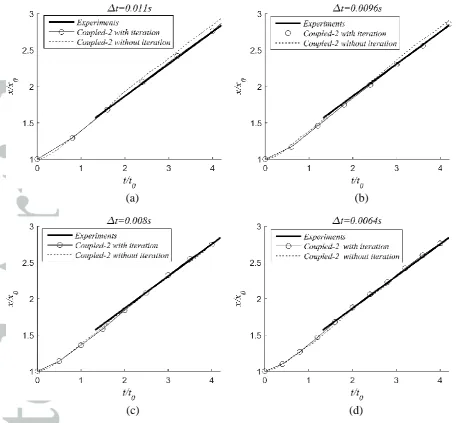
stopping the iteration is set as . Time histories of the heavier fluid front position obtained with and without the iteration are compared with the linear fitted experiment results by [40] in Figure 3, where is the initial front position and , with

. Figure 3 (a) to (d) illustrate the front propagating with decreasing time step length of 0.011s, 0.0096s, 0.008s and 0.0064s, respectively. It can be observed that the results obtained by using iterations with all the time steps agree very well with the experiments. However, without the iteration, the results for the larger time steps can be significantly different from the experimental ones (Figure 3(a)), but the differences can be much reduced when the time step used is sufficiently small (Figure 3(d)).

Figure 3: Comparison of the front time histories of the heavier fluid obtained by using the Coupled-2 approach with or without iteration at time step length of 0.011s, 0.0096s, 0.008s and 0.0064s. ( is

initial front position and )

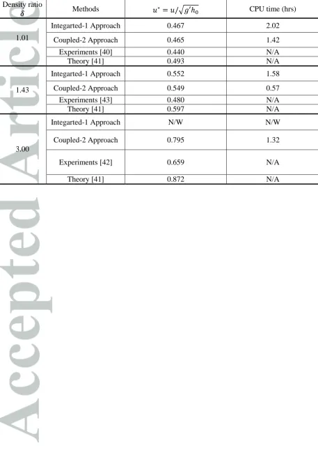
More features of Coupled-2 approach will be demonstrated next by comparing its results with those of Intergated-1 approach. For this purpose, the same case as shown in Figure 2 will be simulated but with different density ratios of 1.01, 1.43 and 3.0 and a fixed time step of 0.0064s. Table 1 presents the calculated dimensionless mean front velocity defined by

reasonably well with the experiments [40]. It is also found that the numerical results lie between the experimental and theoretical values. Although both approaches give similar results for the cases, the Cooupled-2 approach costs less CPU time with the trend that more CPU time may be saved for the higher density ratio. As the density ratio increases to 3.0, the Integarted-1 approach fails to give convergent results whereas the Coupled-2 approach keeps working well and yields the front velocity that is consistent with the experiment [42] and the theory. These tests clearly show that Integarted-1 Approach can only work for fairly low density ratio (close to 1) and fails to deal with high density ratio. The Coupled-2 approach works well for both low and high density ratios. When both approaches work, the Coupled-2 approach is computationally more efficient. Based on this, Coupled-2 approach is preferred.

5.

Validation and numerical results

In this section, several cases will be considered to validate the two-phase MLPG_R method and to investigate the convergence properties of the method. The density ratio will vary from 1.01 to 1000. The Coupled-2 approach will be employed.

5.1. Gravity current flow

The schematic setup for this case is similar to that in Figure 2. In this section, the parameters are selected based on an experiment in [40], in which , and

_{, with a density ratio of 1.048 (the heavier to the lighter), and .}

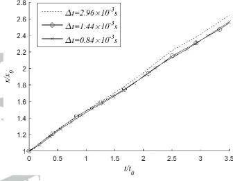
Convergence tests of time step are first carried out. For this purpose, the time step length is chosen as , and with a fixed particle distance of in both directions. Figure 4 illustrates the comparison of the leading front of the heavier fluid obtained by using different time steps. It can be seen that little difference is observed between the results of and , which corresponds to Courant Numbers ( ) of 0.038 and 0.066, respectively.

Figure 4: Comparison of the leading front time histories of the heavier fluid obtained by using different time steps.

In order to investigate how the results vary with different initial particle distances, the cases with a fixed Courant Number of 0.038 but different number of particles are also considered with , , and corresponding to , ,

Figure 5: Comparison of the leading front time histories of the heavier fluid obtained by using different initial particle distances.

Figure 6: Pressure fields at t=10.7s. The density ratio is 1.048 and the setup follows one experiment in [40]. The length scale is non-dimensionalised by the filling depth.

It has been reported in [40,42,43] that, despite changing the initial setup (e.g. ), the non-dimensional velocity ( ) of the heavier fluid front largely keeps constant and the constant does not significantly vary with the density ratio if it is not larger than 1.4 [43]. This character is demonstrated by more tests with different density ratios (1.048, 1.1 and 1.3) carried out with a new setup of and . To simulate these cases, the initial particle distance is selected as 0.01m with the courant number chosen as 0.05 to determine the time step. Figure 7 illustrates the time histories of dimensionless leading front of the heavier fluid obtained by the experiments [40] for the cases with slightly different density ratios (1.01, 1.02 and 1.04), and by two-phase MLPG_R method proposed in this paper for the cases with density ratios of 1.01, 1.048, 1.1 and 1.3. One can find that the front time histories of the experiments and the two-phase MLPG_R method are almost a straight line implying a constant non-dimensional velocity. One can also find that they are correlated very well with each other. This is consistent with the conclusion of [43] that the non-dimensional velocity does not vary significantly when the ratio is less than 1.4.

Figure 7: The time histories of the dimensionless leading front of the heavier fluid obtained by the experiment [40], and by two-phase MLPG_R method for the cases with density ratio of 1.01 1.048, 1.1 and 1.3.

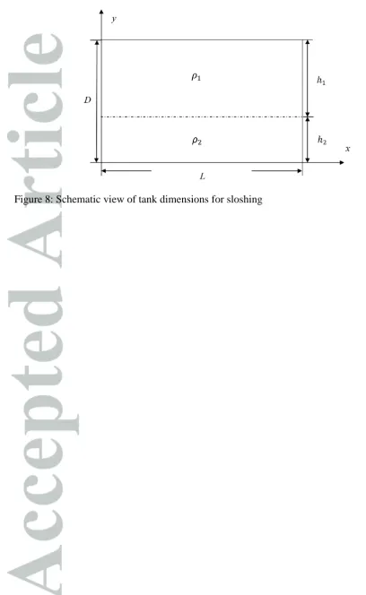
Figure 8: Schematic view of tank dimensions for sloshing

5.2. Sloshing with small amplitudes

through the interface and continuous velocity normal to the interface. The velocity potentials ( ) and interface elevation ( ) in their solution are given by

₍₂₉₎ where (30) (31) where

, and

and

(32)

The pressure in the two liquid domains is derived by means of the linearized Bernoulli equation and is expressed as

(33)

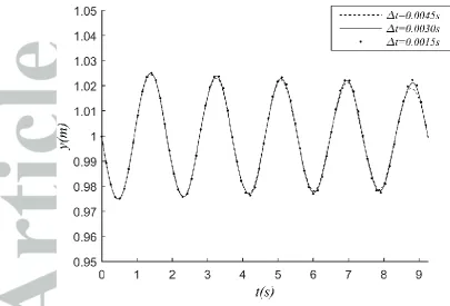
In numerical tests, an initial velocity potential is given at the time when across the tank. Then the fluids start to move. The dimensions of the tank are chosen as , , the filling rate of the fluids is and the density ratio varies. The amplitude is set to be . Time step tests are first carried out with an initial particle distance

corresponding to 55 particles distributed along the depth of with . Time steps of and , corresponding to the courant numbers of 0.027, 0.018 and 0.009, respectively, are used. The maximum velocity in calculating courant number is obtained from Eq. (29), which is . The interface elevations calculated at are shown in Figure 9. It is clear that

_{giving a Courant Number of 0.018 is sufficient to obtain convergent results.}

obtained by different particle numbers (only the results of 0.04m, 0.018m and 0.013m are presented for clarity) and analytical solutions [44]. It indicates that the numerical results converge and have little visible difference from the analytical solutions when . In order to investigate the convergent properties, the error of numerical results is estimated by , where is the analytical solution of wave elevation at at i-th time step, is the corresponding numerical results and is the total number of time steps during the simulation time. Figure 11 shows the variation of the errors with the initial distances between particles for two filling ratios, which are 0.5 in Figure 11(a) and 0.3 in Figure 11 (b), with the different density ratio ranging from 10 to 1000. One can see that the convergent rates in all the cases are close to 2, which is similar to that presented by Zheng, et al. [23] for single phase sloshing.

Figure 9: Interface elevation at x=0.3m calculated using different time steps for a fixed particle number. ( )

Figure 10: Interface elevations at x=0.3m calculated using MLPG_R method and analytical solutions with the analytical solution from [44] ( ).

Figure 11: Numerical errors for density ratios of 10, 50, 200 and 1000 with different particle distances for filling ratio of 0.5(a) and 0.3(b).

Figure 12: Snapshots of pressure distribution at the first quarter ( ) (a) and the third quarter ( ) (b) of the first period with interfaces shown in black.

Figure 13: Pressure distributions along the depth at x=0.3m (a) and x=1.7m (b) at for the case with density ratio of 10. The inset the results near the interface. The analytical solution is from [44].

Figure 14: Pressure specific derivatives in x- and y- directions at x=0.75m (a) and 1.75m (b) at the

time instant of at = 0.75 with the analytical solution from [44]

Figure 15: Natural periods for filling ratios 0.1, 0.12, 0.2, 0.3, 0.5, 0.7 and 0.9, and density ratios of 10 and 1000 with the analytical solution from [44].

To demonstrate the performance of the newly developed method in different ways, Figure 15 shows the comparison of natural periods between numerical and analytical solutions for the cases with the density ratio = 10 and 1000. The agreement between them can be considered as excellent, not only for small density ratio but also for large density ratios.

It is noted that if Eq. (25) that just imposes the pressure continuity would have been used, the acceptable agreement with analytical solution could only be achieved for small density ratio, and the behaviour of the pressure specific derivatives is very different from the analytical solution even when the density ratio is just 1.25 according to our tests.

5.3. Water-air sloshing with strong nonlinearity

Here the two-phase MLPG_R method is further validated using air-water sloshing in the cases with strong nonlinearity. The tank is the similar to that illustrated in Figure 8 with the density ratio of (approximately the ratio of water to air) and with the other parameters set as the same as in [36], i.e., , and . The tank is excited by a periodic horizontal motion of , where the amplitude is

and the frequency is (corresponding to the period of 1.3s). In the simulation, the coordinate system is fixed on the moving tank with the inertial force added in the equation.

Time step lengths of , and (corresponding to courant number of 0.03, 0.06 and 0.09) are tested with a fixed initial particle distance of 0.004m. Water-air interface snapshots at and obtained by different time steps are compared in Figure 16, with insets at the water jets. The interface differences become invisible by keeping the time step shorter than . Based on the maximum velocity estimated by , the courant numbers corresponding to

Figure 16: Snapshots of interfaces obtained using the time steps of , and

_{at (a) and (b).}

By adopting the courant number of 0.03, initial particle distances of /10, /20 and /30 (corresponding to , and ) are tested. The interface profiles at different time instants are displayed on the right column in Figure 17 and no significant difference between the results is observed, even when the water surface overturns and collapses. The left column of Figure 17 shows the comparison between the images taken during experiments [36] and numerical results of . The images from the experiment are for 0.1T, 0.2T, 0.3T and 0.4T (where T is the wave period), for which the exact time instants are not available. The simulation results given are picked out from the second period of the numerical simulation, in which the sloshing wave becomes strongly nonlinear. During wave breakings, complex topological evolutions of the interface occur when water jets splashes out, which is quite well captured by the method as can be seen from the figure. Reasonable agreement of wave surfaces between the experiment and the simulation can also be observed. Pressure time histories at on the right wall for different initial particle distances are compared with the experiment and shown in Figure 18. As can be seen, the numerical pressure time history is quite smooth without notable spurious fluctuations and correlated well with the experimental data. The convergent rate with respect to the measured pressure is around 1.3, which is lower than that obtained in the case of small amplitude sloshing given above. One of the reasons is that for the sloshing case with a small amplitude, the error is calculated relative to the analytical solution while it is relative to the experimental data here. There are also other reasons that may explain this degradation in the convergent rate, when violent waves and impacts are involved, such as neglecting turbulence, lack of accounting for air compressibility and the roughness of the tank wall during the numerical simulation. Apart from the numerical issues, the experimental measurement of impact pressure is highly variable and the large scattering in the measured data were observed as described in [36]. The influences of above numerical and experimental factors are more significant on the peak pressure, as shown in Fig. 18. The another reason for the deviation in the peak pressure perhaps due to the fact that the pressure measured in experiments by pressure sensor is actually over a small area while the computed value is taken from a point as we did not make any average or smoothing. It is just noted that other methods, such as ISPH and MPS may achieve only a convergent rate less than 1 even for cases without breaking, as reviewed in [29].

Figure 17: Comparison of water-air interface profiles at t=1.43s, 1.56s, 1.69s and 1.82s from (a) to (d). Left column gives experiment photos [36] compared with the simulation of 0.004m. The right column gives MLPG_R results for 0.012m, 0.006m and 0.004m(snapshots in the shape of circle, triangle and square respectively).

Figure 18: Comparison of pressure at on the right vertical wall between the experiments and the numerical simulation of MLPG_R method

particularly with the lighter isolated particles in the heavier fluid. As this paper is focused on presenting main elements associated with the development of the two-phase MLPG_R method, the cases related to isolated particles are left to be discussed in future work.

6.

Conclusion

This paper presents the new development of a two-phase MLPG_R method to simulate 2D flow of two immiscible fluids with small viscosity and negligible interface tension. A novel coupling approach has been proposed to ensure the continuity of pressure and the normal velocity and maintain the true discontinuity of fluids properties across the interface when solving Poisson’s equation for pressure. The coupling between two phases is achieved by a newly formulated pressure equation for interface particles, which forms the algebraic equations for pressure together with discretised Poisson’s equation at inner and rigid wall particles. To solve the algebraic equations, two approaches are proposed and tested. One approach (Integrated-1 Approach) is to solve the pressure equations for different fluids as one system, while the other (Coupled-2 Approach) is to split the whole set equation into two coupled sets and to find the solution by iteration between the two sets. The results showed that both approaches can work well for the cases with low density ratios, where the 2 Approach is more computationally efficient. When the density ratio is high, only Coupled-2 Approach can give right results. Based on this, the Coupled-Coupled-2 Approach is recommended in general cases.

The newly developed two-phase MLPG_R method has been validated by comparing its numerical results with the analytical solution of sloshing for layered fluids, and the experimental data of gravity current and excited water-air sloshing. In the layered sloshing cases, the computational results for wave elevations, natural periods, pressure and specific pressure gradient all agree well with the analytical solutions. In addition, the second order convergent rate is achieved with the density ratio from 1 to 1000 in these cases. In the cases for gravity current, the numerical results are compared with experimental data, and found to be well correlated with the data. In the case for water-air sloshing with strong nonlinearity, the numerical interface profiles and pressure time histories are also in reasonable agreement with experimental ones.

It is however recognised that the assumption on the continuity of pressure at the interface with small viscosity and negligible interface tension may not be sufficient for some applications where both the surface tension and viscosity plays a significant role, which is currently under investigation. Although the result in Figure. 17 has demonstrated that the developed method can potentially be applied to model violent flow with fragmentation, more tests are required to confirm its capacity of modelling such flow.

Acknowledgement:

References

[1] C. W. Hirt and B. D. Nichols, ‘Volume of fluid (VOF) method for the dynamics of free boundaries’, J. Comput. Phys., vol. 39, no. 1, pp. 201–225, 1981.

[2] M. Rudman, ‘Volume-Tracking Methods for Interfacial Flow Calculations’, Int. J. Numer. Methods Fluids, vol. 24, no. 7, pp. 671–691, 1997.

[3] M. Sussman, P. Smereka, and S. Osher, ‘A Level Set Approach for Computing Solutions to Incompressible Two-Phase Flow’, J. Comput. Phys., vol. 114, pp. 146– 159, 1994.

[4] J. A. Sethian and P. Smereka, ‘Level Set Methods for Fluid Interfaces’, Annu. Rev. Fluid Mech., vol. 35, no. 1, pp. 341–372, 2003.

[5] P. Gomez, J. Hernandez, and J. Lopez, ‘On the reinitialization procedure in a narrow-band locally refined level set method for interfacial flows’, Int. J. Numer. Methods Eng., vol. 63, no. 10, pp. 1478–1512, 2005.

[6] M. Sussman and E. G. Puckett, ‘A Coupled Level Set and Volume-of-Fluid Method for Computing 3D and Axisymmetric Incompressible Two-Phase Flows’, J. Comput. Phys., vol. 162, no. 2, pp. 301–337, 2000.

[7] M. Sussman, K. M. Smith, M. Y. Hussaini, M. Ohta, and R. Zhi-Wei, ‘A sharp

interface method for incompressible two-phase flows’, J. Comput. Phys., vol. 221, no. 2, pp. 469–505, 2007.

[8] X. Lv, Q. Zou, Y. Zhao, and D. Reeve, ‘A novel coupled level set and volume of fluid method for sharp interface capturing on 3D tetrahedral grids’, J. Comput. Phys., vol. 229, no. 7, pp. 2573–2604, 2010.

[9] T. Ménard, S. Tanguy, and A. Berlemont, ‘Coupling level set/VOF/ghost fluid methods: Validation and application to 3D simulation of the primary break-up of a liquid jet’, Int. J. Multiph. Flow, vol. 33, no. 5, pp. 510–524, 2007.

[10] E. S. Lee, C. Moulinec, R. Xu, D. Violeau, D. Laurence, and P. Stansby, ‘Comparisons of weakly compressible and truly incompressible algorithms for the SPH mesh free particle method’, J. Comput. Phys., vol. 227, no. 18, pp. 8417–8436, 2008.

[12] A. Shakibaeinia and Y. Jin, ‘MPS mesh-free particle method for multiphase flows’,

Comput. Methods Appl. Mech. Eng., vol. 229–232, pp. 13–26, 2012.

[13] A. Khayyer and H. Gotoh, ‘Enhancement of performance and stability of MPS mesh-free particle method for multiphase flows characterized by high density ratios’, J. Comput. Phys., vol. 242, pp. 211–233, 2013.

[14] J. J. Monaghan and a. Kocharyan, ‘SPH simulation of multi-phase flow’, Comput. Phys. Commun., vol. 87, no. 1–2, pp. 225–235, 1995.

[15] J. Kwon and J. J. Monaghan, ‘Sedimentation in homogeneous and inhomogeneous fluids using SPH’, Int. J. Multiph. Flow, vol. 72, pp. 155–164, 2015.

[16] A. Colagrossi and M. Landrini, ‘Numerical simulation of interfacial flows by smoothed particle hydrodynamics’, J. Comput. Phys., vol. 191, no. 2, pp. 448–475, 2003.

[17] X. Y. Hu and N. a. Adams, ‘A multi-phase SPH method for macroscopic and mesoscopic flows’, J. Comput. Phys., vol. 213, no. 2, pp. 844–861, 2006.

[18] N. Grenier, M. Antuono, a. Colagrossi, D. Le Touzé, and B. Alessandrini, ‘An Hamiltonian interface SPH formulation for multi-fluid and free surface flows’, J. Comput. Phys., vol. 228, no. 22, pp. 8380–8393, 2009.

[19] J. J. Monaghan and A. Rafiee, ‘A simple SPH algorithm for multi-fluid flow with high density ratios’, Int. J. Numer. Methods Fluids, vol. 71, pp. 537–561, 2013.

[20] K. Szewc, J. Pozorski, and J. P. Minier, ‘Spurious interface fragmentation in multiphase SPH’, Int. J. Numer. Methods Eng., vol. 103, no. 9, pp. 625–649, 2015.

[21] X. Y. Hu and N. A. Adams, ‘An incompressible multi-phase SPH method’, J. Comput. Phys., vol. 227, no. 1, pp. 264–278, 2007.

[22] X. Y. Hu and N. A. Adams, ‘A constant-density approach for incompressible multi-phase SPH’, J. Comput. Phys., vol. 228, no. 6, pp. 2082–2091, 2009.

[23] S. D. Shao, ‘Incompressible smoothed particle hydrodynamics simulation of multifluid flows’, Int. J. Numer. Methods Fluids, vol. 69, pp. 1715–1735, 2012.

Comput. Phys., vol. 309, pp. 129–147, 2016.

[25] H. Ikari, A. Khayyer, and H. Gotoh, ‘Corrected higher order Laplacian for enhancement of pressure calculation by projection-based particle methods with applications in ocean engineering’, J. Ocean Eng. Mar. Energy, vol. 1, no. 2013, pp. 361–376, 2015.

[26] H. F. Schwaiger, ‘An implicit corrected SPH formulation for thermal diffusion with linear free surface boundary conditions’, Int. J. Numer. Methods Eng., vol. 75, no. 6, pp. 647–671, 2008.

[27] X. Zheng, Q. W. Ma, and W. Y. Duan, ‘Incompressible SPH method based on Rankine source solution for violent water wave simulation’, J. Comput. Phys., vol. 276, pp. 291–314, 2014.

[28] S. J. Lind, R. Xu, P. K. Stansby, and B. D. Rogers, ‘Incompressible smoothed particle hydrodynamics for free: surface flows: A generalised diffusion-based algorithm for stability and validations for impulsive flows and propagating waves’, J. Comput. Phys., vol. 231, no. 4, pp. 1499–1523, 2012.

[29] Q. W. Ma, Y. Zhou, and S. Yan, ‘A review on approaches to solving Poisson’s

equation in projection-based meshless methods for modelling strongly nonlinear water waves’, J. Ocean Eng. Mar. Energy, vol. 2, no. 3, pp. 279–299, 2016.

[30] Q. W. Ma, ‘MLPG Method Based on Rankine Source Solution for Simulating Nonlinear Water Waves’, C. - Comput. Model. Eng. Sci., vol. 9, no. 2, pp. 193–209, 2005.

[31] Q. W. Ma and J. T. Zhou, ‘MLPG_R Method for Numerical Simulation of 2D BreakingWaves’, C. - Comput. Model. Eng. Sci., vol. 43, no. 3, pp. 277–303, 2009.

[32] V. Sriram and Q. W. Ma, ‘Improved MLPG_R method for simulating 2D interaction between violent waves and elastic structures’, J. Comput. Phys., vol. 231, no. 22, pp. 7650–7670, 2012.

[33] R. P. Fedkiw, T. Aslam, B. Merriman, and S. Osher, ‘A Non-oscillatory Eulerian Approach to Interfaces in Multimaterial Flows (the Ghost Fluid Method)’, J. Comput. Phys., vol. 152, no. 2, pp. 457–492, 1999.

[34] S. J. Lind, P. K. Stansby, B. D. Rogers, and P. M. Lloyd, ‘Numerical predictions of water–air wave slam using incompressible–compressible smoothed particle

[35] S. Yan and Q. W. Ma, ‘Numerical simulation of interaction between wind and 2D freak waves’, Eur. J. Mech. B/Fluids, vol. 29, no. 1, pp. 18–31, 2010.

[36] Z. R. Kishev, C. Hu, and M. Kashiwagi, ‘Numerical simulation of violent sloshing by a CIP-based method’, J. Mar. Sci. Technol., vol. 11, no. 2, pp. 111–122, 2006.

[37] S. Koshizuka and Y. Oka, ‘Moving-particle semi-implicit method for fragmentation of incompressible fluid’, Nuclear science and engineering, vol. 123, no. 3. pp. 421–434, 1996.

[38] E. G. Flekkoy, P. V. Coveney, and G. De Fabritiis, ‘Foundations of dissipative particle dynamics’, Phys. Rev. E. Stat. Phys. Plasmas. Fluids. Relat. Interdiscip. Topics, vol. 62, no. 2, p. 2140, 2000.

[39] Y. Zhou and Q. W. Ma, ‘A New Interface Identification Technique Based on Absolute Density Gradient for Violent Flows’, C. - Comput. Model. Eng. Sci., 2016. In print

[40] J. W. Rottman and J. E. Simpson, ‘Gravity currents produced by instantaneous releases of a heavy fluid in a rectangular channel’, J. Fluid Mech., vol. 135, pp. 95–110, 1983.

[41] J. J. Keller and Y. P. Chyou, ‘On the hydraulic lock-exchange problem’, J. Math. Phys., vol. 42, no. November, pp. 874–910, 1991.

[42] H. P. Grobelbauer, T. K. Fannelop, and R. E. Britter, ‘The progradation of intrusion fronts of high density ratios’, J. Fluid Mech., vol. 250, pp. 669–687, 1993.

[43] R. J. Lowe, J. W. Rottman, and P. F. Linden, ‘The non-Boussinesq lock-exchange problem. Part 1. Theory and experiments’, J. Fluid Mech., vol. 537, pp. 101–124, 2005.

Table 1: Comparison of the mean velocity of the heavy fluid front and CPU time using different methods with density ratio of , 1.43 and 3.0. (N/A: Not available; N/W: Not working) Density ratio

Methods CPU time (hrs)

1.01

Integarted-1 Approach 0.467 2.02

Coupled-2 Approach 0.465 1.42

Experiments [40] 0.440 N/A

Theory [41] 0.493 N/A

1.43

Integarted-1 Approach 0.552 1.58

Coupled-2 Approach 0.549 0.57

Experiments [43] 0.480 N/A

Theory [41] 0.597 N/A

3.00

Integarted-1 Approach N/W N/W

Coupled-2 Approach 0.795 1.32

Experiments [42] 0.659 N/A

(a) (b)

(c) (d)

Figure 3: Comparison of the front time histories of the heavier fluid obtained by using the Coupled-2 approach with or without iteration at time step length of 0.011s, 0.0096s, 0.008s and 0.0064s. ( is

(a) (b)

(a) (b)

(a) (b)

(a)

(b)

Figure 14: Pressure specific derivatives in x- and y- directions at x=0.75m (a) and 1.75m (b) at the

(a) (b)

Figure 16: Snapshots of interfaces obtained using the time steps of , and

(b)

(c)

(d)

Figure 17: Comparison of water-air interface profiles at t=1.43s, 1.56s and 1.69s from (a) to (c). Left column gives experiment photos [33] compared with the simulation of 0.004m. The right

MLPG_R method for modelling 2D flows of two immiscible fluids

Yan Zhou, Q.W. Ma* and S. Yan