City, University of London Institutional Repository
Citation
:
Glock, C.H. & Ries, J.M. (2013). Reducing lead time risk through multiple sourcing: the case of stochastic demand and variable lead time. International Journal of Production Research, 51(1), pp. 43-56. doi: 10.1080/00207543.2011.644817This is the accepted version of the paper.
This version of the publication may differ from the final published
version.
Permanent repository link:
http://openaccess.city.ac.uk/17126/Link to published version
:
http://dx.doi.org/10.1080/00207543.2011.644817Copyright and reuse:
City Research Online aims to make research
outputs of City, University of London available to a wider audience.
Copyright and Moral Rights remain with the author(s) and/or copyright
holders. URLs from City Research Online may be freely distributed and
linked to.
City Research Online: http://openaccess.city.ac.uk/ [email protected]
1
Reducing lead time risk through multiple sourcing: The case of stochastic demand and variable lead time
Christoph H. Glock
Chair of Business Management and Industrial Management, University of Wuerzburg ([email protected])
Jörg M. Ries
Chair of Business Management and Industrial Management, University of Wuerzburg ([email protected])
Abstract: This paper studies a buyer sourcing a product from multiple suppliers under stochas-tic demand. The buyer uses a (Q,s) continuous review, reorder point, order quantity inventory control system to determine the size and timing of orders. Lead time is assumed to be deter-ministic and to vary linearly with the lot size, wherefore lead time and the associated stockout risk may be influenced both by varying the lot size and the number of contracted suppliers. This paper presents mathematical models for a multiple supplier single buyer integrated inven-tory problem with stochastic demand and variable lead time and studies the impact of the de-livery structure on the risk of incurring a stockout during lead time.
Keywords: Variable lead time; Supply chain coordination; Supplier selection; Multiple sourc-ing; Delivery structure; Integrated inventory
Introduction
The management of risks in supply chains has received increased attention among both practi-tioners and researchers in recent years. Reasons for the growing importance of risk manage-ment are manifold and originate from various trends that enhance the exposure of supply chains to risks. Business concepts, such as outsourcing initiatives, global sourcing, reduced supplier bases and inventory buffers aim to improve the performance of the supply chain in a stable environment, but also increase its vulnerability to potential disruptions (see, e.g., Norman and Jansson, 2004; Hendricks and Singhal, 2005a). Empirical studies indicate that companies suf-fering from supply chain disruptions experience significant declines in operating performance (Hendricks and Singhal, 2005b) as well as lower stock returns and higher equity risks relative to their industry benchmarks (Hendricks and Singhal, 2005a), which illustrates the importance of controlling risks in the supply chain. To mitigate the impact of disruptions associated with various types of risks, it is necessary to coordinate the material flows in the network of organ-isations and to collaborate with upstream and downstream members of the supply chain to improve operations and to ensure continuity (Tang, 2006). A continuous flow of materials thereby depends on the sourcing structure, i.e. on the composition of the supplier base and the coordination of deliveries, as well as on the allocation of inventories along the supply chain.
2 Various publications addressed the determination of safety stocks in cases where customer de-mand and/or lead times are uncertain. In this context, many authors studied multiple sourcing as a means to reduce supply risks and showed that in case of stochastic lead times, contracting multiple suppliers is an appropriate measure to reduce the risk of a stockout in the period be-tween the issue and receipt of an order. Sculli and Wu (1981), for instance, considered a con-tinuous review inventory model with two suppliers under normally distributed lead times and assumed that the replenishment quantity is split into two portions, which are ordered simulta-neously at the suppliers. In this case, the effective lead time is the minimum of the set of random variables representing the lead time of each supplier, which helps to reduce stockout risk and consequently expected total costs. Hayya et al. (1987) conducted a simulation study to estimate the effects of splitting orders between two suppliers on stockout risk and average inventory. Sculli and Shum (1990) extended the model to include multiple suppliers, and Kelle and Silver (1990a,b) considered the case of splitting replenishment orders among two or more suppliers with identical lead times following a Weibull distribution. Ramasesh et al. (1991, 1993) pro-vided further extensions to the model and studied uniform and exponential lead times as well as identical and nonidentical suppliers. The case where demand and lead times are both sto-chastic was analysed by Lau and Zhao (1993), who studied the impact of order splitting among two suppliers on reducing stockout risk. The authors showed that order splitting lowers cycle inventory and that contracting a second supplier with a larger mean lead time than the first supplier may not necessarily increase expected total costs. Chiang and Benton (1994) provided a comparative analysis of single and dual sourcing practices under normally distributed demand and shifted-exponential lead times. Numerical studies indicated that dual sourcing provides a higher service level and results in higher order quantities than single sourcing. A study of order splitting from an inventory perspective under a generic lead time distribution can be found in Hill (1996), who showed that multiple sourcing reduces average stock levels. Ganeshan et al. (1999) investigated the benefits of splitting orders between a reliable and an unreliable supplier that offers a purchase price discount. Cost comparisons were used to derive the discount rates the unreliable supplier needs to provide to make splitting worthwhile for different order allo-cations. Order splitting between two suppliers with different lead time characteristics was also studied by Kelle and Miller (2001), who investigated its effects on stockout risk. They showed that dual sourcing can provide lower stockout risks even for a second supplier with an inferior delivery performance, and that an optimal order split leads to lower stockout risks in the case of different lead time characteristics, as compared to an equal split. Ryu and Lee (2003) con-sidered dual sourcing models with lead time expedition cost functions and showed that these investments lead to significant savings. Sajadieh and Eshghi (2009) extended dual sourcing models and introduced order quantity-dependant lead times and unit purchase prices. Numeri-cal results indicated that purchase quantity discounts decrease savings obtained from order splitting and result in unequal splits even if suppliers are identical. Furthermore, order splitting seems to be favourable when delivery characteristics are similar. A comprehensive overview of different alternatives of splitting orders between multiple suppliers can further be found in Thomas and Tyworth (2006).
3 quantity as decision variables and studied the cases of a linear and an exponential lead time crashing cost-function. Ouyang et al. (1996) introduced another extension and include short-ages in the model. They assumed that a certain fraction of the demand during the stockout period is backordered and that the remaining fraction results in lost sales. Chandra and Grabis (2008) assumed that reduced lead time is accompanied by increased procurement costs due to premium charges imposed by the supplier or higher transportation costs, and studied the inter-dependencies between a reduction in stockout risk and an increase in procurement costs. Jha and Shanker (2009) formulated an integrated inventory model with controllable lead time for items with a constant decay rate and optimised order quantity, lead time and the number of shipments under a service level constraint. Other authors studied lead time reduction in inven-tory models with stochastic demand and permitted further model parameters to be varied as well, such as setup costs or product quality. Examples are the models of Ouyang and Chang (2002), Ben-Daya and Hariga (2003), Zequeira et al. (2005), and Pan and Lo (2008). A contin-uous review model with variable, lot size-dependent lead time can finally be found in Ben-Daya and Hariga (2004) and Glock (2009, In Press a). The authors assumed that lead time varies linearly with the lot size and studied the impact of a variation in the lot size on the safety stock and the expected total costs of the system.
A closer look at the literature reviewed above reveals that previous research has mainly focused on analysing multiple sourcing in cases where lead time is stochastic, but that the case where lead time is deterministic and varying with the lot size has thus far not been studied in a setting with multiple suppliers. This is insufficient inasmuch as many real world scenarios exist where stochastic influences on the replenishment lead time are negligible (for example if buyer and supplier are located in close geographic proximity), but where the length of the lead time is primarily influenced by the quantity ordered (for example in serial production processes). If demand during lead time is assumed to be stochastic in such a setting, the buyer may influence stockout risk by splitting the replenishment order on multiple suppliers and by thus reducing the length of the individual lead times, as well as by varying order quantities and replenishment policies. To close this gap, a single item integrated inventory system consisting of multiple suppliers and a single buyer who faces stochastic demand and splits the replenishment orders among the suppliers is studied in this paper. Our work focuses explicitly on the total costs of the supply chain under study (for reviews of so-called integrated inventory models see Goyal and Gupta, 1989; Ben-Daya et al., 2008; Glock, In Press b) to examine how supply chain op-erations and the management of risks can be improved through coordination and collaboration among the supply chain partners (Tang, 2006; Cao et al., 2010). This also enables us to assess the impact of individual decisions on the risk and performance of the supply chain partners and helps to develop strategies that improve the competitive position of the supply chain as a whole.
The remainder of the paper is organised as follows: In the next section, the article outlines the assumptions and definitions which are used in the paper. Accordingly, Section 3 develops for-mal models which consider stochastic demand and variable lead time in a system with multiple suppliers. Section 4 contains a numerical study and Section 5 concludes the article.
Problem description
4 subsequent stage or the customer after its completion (note that this scenario is studied in many papers, see e.g. Kim and Benton, 1995; Ben-Daya and Hariga, 2004; Hsiao 2008; Glock 2009, In Press a, among others). However, we note that other production processes might be associ-ated with different functional forms, such as a step-wise lead time-function for example, which could be representative for production processes where each batch needs a certain production time regardless of the number of units in the batch, for instance in case products are heated in an oven or treated in an immersion bath. The replenishment quantity is split evenly among the suppliers, who initiate production upon receipt of the order and deliver the production quantity to the buyer after the lead time L has elapsed. To reduce the complexity of our model, we assume that the suppliers are homogeneous, i.e. that all problem parameters are identical for the suppliers (note that this assumption is not uncommon in the literature, cf. for example Kelle and Silver, 1990b; Ramasesh et al.,1991; Chiang and Benton, 1994; Hill, 1996; Ganeshan, 1999). This scenario is representative for a variety of industries, for example for industries that produce standard mechanical components for automotive manufacturers or for commodity markets (see for example Oladi and Gilbert, 2009; Smith and Thanassoulis, 2008). Further, we consider two alternative delivery structures which are discussed in Rosenblatt et al. (1998), Park et al. (2006), Kim and Goyal (2009), Kheljani et al. (2009), and Glock (2011a, 2011b), among others, and which are illustrated exemplarily in Figure 1. In the first case (cf. part a) of Figure 1), which we term simultaneous deliveries in the following, the suppliers deliver at the same time to the buyer. In the second case (cf. part b) of Figure 1), which we term sequential deliveries, the suppliers deliver alternately, such that a shipment reaches the buyer exactly when the shipment of the supplier who has delivered previously is expected to have been used up (note that the dashed line in Figure 1 represent inventory build-up with a lower production rate).
--- Figure 1 ---
Apart from the assumptions already stated, we assume the following hereafter:
1. Demand per unit of time follows a normal distribution with mean D and standard deviation
σ. Thus, demand during lead time, x, has the probability density function f(x) with mean
DL(Q,n) and standard deviation 𝜎√𝐿(𝑄, 𝑛).
2. Lead time is proportional to the lot size produced by the supplier and consists of processing time and a fixed delay due to transportation or nonproductive time (see Ben-Daya and Hariga, 2004). Lead time may thus be calculated as L(Q,n) = Q/(nP)+b.
3. Unsatisfied demand at the buyer is backordered.
4. The focus is on the total costs of the system, since we assume that the suppliers will pass on savings or increases in cost to the buyer. Transfer payments between the suppliers and the buyer are not considered.
5 In addition, the following terminology is used:
A = ordering costs per order
a = cost parameter of the supplier handling cost function
b = fixed delay factor
C(n) = supplier handling and material receiving costs
D = demand rate in units per unit time
hb = unit inventory carrying charges per unit of time at the buyer
hv = unit inventory carrying charges per unit of time at the suppliers
K = setup and transportation costs per production lot at the supplier
L = lead time
n = number of suppliers
nmin = minimum number of suppliers the buyer needs to contract 𝑛̂ = nmin– 1
k = safety factor
p = inverse production rate, i.e. p = 1/P P = production rate in units per unit time
π = backorder costs per unit backordered
Q = order quantity
q = production quantity of supplier i r = reorder point
S = safety stock
t = cost parameter of the supplier handling cost function
σ = standard deviation of demand
x = lead time demand
Y = receiving costs per delivery
Definitions
[ε] denotes rounding a non-integer value ε to the nearest integer
ε denotes rounding a non-integer value ε up to the next integer |ε| the absolute value of ε, i.e. 2
SEQ model that considers sequential deliveries from the suppliers SIM model that considers simultaneous deliveries from the suppliers
Model development
Simultaneous deliveries
First, we consider the case where the buyer places orders simultaneously at the suppliers. In this case, it can be easily shown that it is optimal to order an equal quantity at each of the suppliers. If q denotes the production quantity of supplier i and n the number of suppliers, it follows that q(Q,n)= Q/n. As can be seen in Figure 1, the suppliers initiate production with a delay of b time units after receipt of the order and deliver a batch of size Q/n to the buyer as soon as the batch has been finished. Inventory per lot at supplier i may thus be calculated as
Q2/(2Pn2). The total costs of supplier i are consequently given as:
(1)
Q KD Pn
QDhv 2
2
6 may be expressed as Q/2 + S. The backorder costs per cycle may be derived by calculating the expected shortage, which is:
(2)
r x r f x dx
n Q L r
s , ,
The sum of inventory carrying costs, ordering costs, supplier handling and material receiving costs and backorder costs per unit time amounts to:
(3)
s
r L
Q n
Q D S Q h Q D n C Ab , ,
2
The system’s expected total costs per unit of time may now be calculated as the sum of (1) and (3), whereby (1) has to be summed up over all suppliers:
(4)
s
r L
Q n
Q D Sh Pn Dh h Q Q D n C nK A ETC b v
b , ,
2
Before deriving a solution for the model, it is beneficial to substitute the reorder point r in (4) by the safety factor k. This can be done by transforming the normal probability density function in (2) into a standard normal probability density function and by substituting r by k√L(Q,n)
+ , with being the expected demand during lead time, DL(Q,n). The safety stock, in turn, equals the difference between the reorder point and the expected demand during lead time, r –
DL(Q,n). Using the expression introduced above leads to:
(5) Sk L
Q,n
k pq
Q,n
bIt follows that:
(6)
pq
Q n b
kQ D h b n Q pq k Pn Dh h Q Q D n C nK A
ETC v b
b
, , 2
where ψ(k)=∫ (k∞ z – k)f(z)dz and f(z) is the standard normal probability density function. To simplify notation, let G(n) = A + nK + C(n) and H(n) = hb +
Dhv
Pn. Consequently, the expected
total costs can be rewritten as:
(7)
pq
Q n b
kQ D h b n Q pq k n H Q Q D n G
ETC , b ,
2
When searching for optimal values for Q, k and n, it has to be considered that the delivery quantity needs to be large enough to exceed the reorder point reduced by the safety stock, i.e.
7 planned shortages may occur, since the suppliers are assumed to deliver after the buyer is ex-pected to have run out of material. As the production time of supplier i depends on both Q and
n, and the expected consumption time of the buyer is dependent on Q, it is obvious that the condition formulated above has to be considered when finding values for Q and n.
Hadley and Whitin (1963) and Ben-Daya and Hariga (2004) suggested that an optimal solution to their models can be found by calculating partial derivatives of the respective objective func-tions with respect to Q and k. However, since the values of Q and n are restricted in the present case, it would be necessary to derive the Karush-Kuhn-Tucker (KKT) conditions to guarantee optimality (see e.g. Hillier and Lieberman, 2001). Since the objective function (7) is too com-plex to derive the KKT conditions and since convexity of (7) in Q cannot be proved, we used the NMinimize-Function of the software package Mathematica 7.0 (Wolfram Research, Inc.) to derive a solution for the problem. The NMinimize-function contains several methods for solving constrained and unconstrained global optimisation problems, such as genetic algo-rithms, simulated annealing or the simplex method. Using a standard software package has several advantages, especially for practitioners. On the one hand, results may be easily obtained and reproduced without the need to develop sophisticated solution mechanisms, and further the user may benefit from advances in optimisation theory which may be included in future release versions of the software package. Numerical results for the problem are presented in Section 4.
Sequential deliveries
As can be inferred from Figure 1, for a given lot size and a given number of suppliers, the total costs of supplier i are identical for both the cases of simultaneous and sequential deliveries. Consequently, the total costs of supplier i equal those given in (1). However, two major aspects are different in this model as compared to the case of simultaneous deliveries. First, for given values of Q, n, and k, the average inventory at the buyer is reduced to Q/(2n) + S due to the fact that the buyer does not receive deliveries of size Q, but more frequent deliveries of size Q/n, which reduces the expected maximum inventory in the system. Second, the expected shortage and total shortage costs may have to be calculated differently in this case, depending on the values of P, D,n and b. First, consider the case where Q/(nD) Q/(nP)+b. In this case, as can be seen in part b) of Figure 1 (cf. the bold lines), an order is placed at one of the suppliers as soon as the inventory level reaches the reorder point. The supplier initiates production after a delay time b and delivers the order once the production lot q has been completed. As soon as the inventory level reaches the reorder point again, an order is placed at one of the other sup-pliers. It is obvious that in this case, both safety stock and expected shortages may be calculated as in expression (7). Thereby the expected shortage, which occurs in every delivery cycle, has to be multiplied with n. However, in case Q/(nD) < Q/(nP)+b (cf. the dotted lines in part b) of Figure 1), the problem arises that the time to produce a lot of size q at one of the suppliers exceeds the average consumption time of this lot. To avoid excessive shortages, it is necessary to place an order at the suppliers in an earlier consumption cycle, which results in overlapping production phases. The major problem with this practice is that the model of Hadley and Whitin (1963) requires in its original form that there is never more than one order outstanding at a time, wherefore further assumptions are necessary to assure that the formulation introduced above may still be used in this case. As was shown by Hadley and Whitin (1963), their approx-imation is applicable for any number of orders outstanding if the probability of the lead time demand exceeding r + (nmin–1)Q/n is low, which implies that after the arrival of a shipment,
8 point. Further, it is required that the backorder costs are independent of the length of the stock-out period and that the contribution of the expected number of backorders to the inventory carrying charge is negligible. To assure that the approximation introduced above may still be used in case Q/(nD) < Q/(nP)+b, we assume in the following that these prerequisites are met.
The following example illustrates how the expected number of backorders may be calculated. Assume that the buyer orders a lot of size q at supplier i at time 0. Supplier i initiates production after the delay time b and finishes the lot at time pq + b. However, due to q/D < q/P+b, it is necessary that the buyer receives further shipments during the lead time L to avoid planned shortages. The number of deliveries the buyer needs to receive during the lead time L to avoid planned shortages may be calculated as n̂ =nmin− 1, whereby nmin is the minimal number of
suppliers the buyer needs to contract. nmin, in turn, may be calculated by considering that the
production quantity of supplier i needs to be large enough to exceed the reorder point reduced by the safety stock, i.e. R – S < Q/n. It follows that:
(8)
Q nb P D nmin 1
The actual nmin is the smallest integer number for which inequation (8) is satisfied. The expected
shortage may now be determined by calculating the expected demand during lead time exceed-ing the reorder point r and the number of shipments the buyer receives during the lead time:
(9)
Z
r x Z r f x dx
n Q L r
s , , where Z = q(Q,n)𝑛̂
Note that in case Q/(nD) ≥ Q/(nP)+b, n̂ equals 0 and expression (9) reduces to (2). The safety stock now equals the sum of the reorder point and the delivery quantity Z, reduced by the expected demand during lead time, i.e. S = r + Z – DL(Q,n). Considering that r = k√𝐿(𝑄, 𝑛)
+ – Z, it becomes obvious that the safety stock equals the one given in (5).
The system’s expected total costs for both the cases Q/(nD) ≥ Q/(nP)+b and Q/(nD) <
Q/(nP)+b may now be calculated as follows:
(10)
pq
Q n b
kQ nD h b n Q pq k Pn Dh n h Q Q D n C nK A
ETC b v b
, , 2
Substituting G(n) = (A + nK + C(n)) and H(n) = (ℎ𝑛𝑏+Dhv
nP), the expected total costs can be
rewritten as:
(11)
pq
Q n b
kQ nD h b n Q pq k n H Q Q D n G
ETC , b ,
2
To find a solution for Q, k and n that minimises the expected total costs, we again used the NMinimize-function of the software package Mathematica 7.0 and assumed that the condition
9
Effects of the decision variables on the safety stock and risk
In the models developed in this paper, two of the buyer’s decision variables directly influence lead time and thus the risk of incurring a stockout, which also affects safety stock: the order quantity Q and the number of suppliers n. Furthermore, the buyer has to decide on the desired service level, which is determined by the safety factor and the alternative delivery structures, and which, in turn, affects available stocks and stockout risk. The effect of the variables on the safety stock of the system and the risk of incurring a stockout during lead time will be discussed in the following:
The impact of a variation of Q on the level of safety stock kept at the buyer for the case of a lot size-dependent lead time has been analysed by Kim and Benton (1995). The authors differen-tiated between an order frequency effect and a lead time effect: The order frequency effect refers to the fact that a reduction in Q leads to an increase in the order frequency D/Q, which in turn exposes the system to the risk of stockouts more often. Consequently, for a fixed lead time, a reduction in the lot size increases the safety stock S to control the occurrence of stock-outs, and vice versa. The lead time effect, in contrast, describes a negative correlation between the length of the lead time and the uncertainty in demand during lead time. Thus, with a de-creasing lot size, lead time is shortened, which leads to a lower demand uncertainty and a lower safety stock for a given order frequency. The interrelations described by Kim and Benton (1995) are also valid for the model developed in this paper.
Taking a closer look at the number of suppliers, an increase in n entails a smaller production lot size q at supplier i if Q remains constant. This, in turn, leads to a similar lead time effect than the one described above. In case of model SIM, the order frequency effect is not directly influenced by a variation in the number of suppliers if the order quantity Q remains constant. In model SEQ, however, an increase in the number of suppliers reduces the order cycle, which leads to a higher order frequency and the order frequency effect described above. Moreover, since an increase in n reduces inventory at the suppliers and at the buyer in case of a sequential delivery, we may assume that the order quantity Q is increased, which again leads to the order frequency effect.
The safety factor k, in turn, also influences safety stock and the risk of running out of stock. If the system aims on reducing the probability of incurring a stockout during lead time, a higher safety stock needs to be kept, which increases k. Ceteris paribus, this leads to higher inventory in the system, and thus induces the order frequency and lead time effect.
Finally, it is obvious that also the delivery structure influences the inventory position of the buyer. For a given lead time, a given safety factor and a given number of suppliers, sequential deliveries lead to lower inventory carrying costs at the buyer. This in turn favours higher order quantities, which may indirectly bring about the order frequency and lead time effects.
10
Simulation study
An analysis of equations (6) and (10) indicates that sequential deliveries result in lower costs for cycle inventory, at the expense of potentially higher shortage costs as compared to simul-taneous deliveries, which may have a significant impact on sourcing decisions and the associ-ated stockout risk. Before analysing the effects of the problem parameters and the inventory structure on the expected total cost and the risk in detail, a simple example illustrates the be-haviour of the models developed in this paper. Consider a two-stage supply chain with the input parameters given in Table 1. Computing order quantities, numbers of contracted suppliers, ser-vice levels and expected total costs for both supply modes, sequential deliveries lead to higher order quantities as well as a higher number of suppliers. Further, sequential deliveries result in lower costs and a higher service level as compared to simultaneous deliveries (cf. Table 2).
--- Table 1 ---
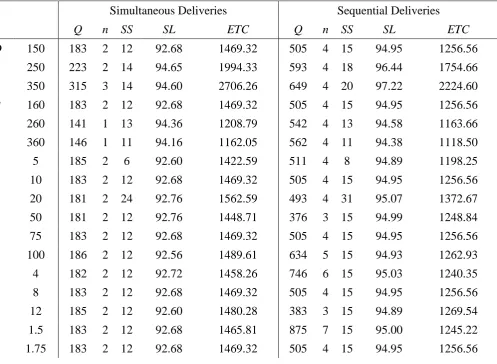
The effects of varying the different input parameters on the order quantity, the number of sup-pliers, the service levels and the expected total costs for both supply modes are illustrated in Table 2. Higher demand rates result in increasing order quantities, safety stocks and service levels for both supply modes which is associated with higher expected total costs. Higher pro-duction rates, in contrast to demand rates, lead to lower costs, especially for simultaneous de-liveries, but have mixed effects on the other parameters. For sequential dede-liveries, the order quantity increases, whereas safety stock and service level decrease. In the case of simultaneous deliveries, similar effects can be observed for a constant number of suppliers. A higher standard deviation of demand induces higher safety stocks and higher total costs. An increase in the ordering costs leads to increasing order quantities and higher total costs especially for simulta-neous deliveries and an increasing number of suppliers for sequential deliveries. The results for various parameters of supplier handling costs show that cost increases have only little in-fluence on simultaneous deliveries, but that they result in smaller order quantities and a de-creasing number of suppliers for sequential deliveries where usually more suppliers are used and consequently supplier handling costs are more important. Higher receiving costs also have little influences on simultaneous deliveries where all partial deliveries are stored at the same time, but lead to higher order quantities and costs in the case of sequential deliveries.
--- Table 2 ---
Lower setup and transportation costs for suppliers lead to smaller lot sizes and lower expected total costs for both delivery modes. Increasing inventory holding costs induce lower order quantities, lower safety stocks and higher expected total costs. Service levels, however, decline if the buyer’s inventory holding costs increase and rise if the suppliers’ inventory holding costs increase. Higher backorder costs lead to slightly lower order quantities and higher safety stocks, service levels and costs. Increasing delay time induces higher cycle and safety inventories as well as increases in expected total costs.
11 suppliers deliver simultaneously to the buyer (model SIM) in 99.9% of the problem instances we studied, and that sequential deliveries led to 16.94% lower expected total costs on average as compared to the other delivery structure. However, as Table 4 illustrates, model SIM may also lead to better results than model SEQ. The backorder quantity, which we use as a measure for the risk incurred in the system (for alternative measures to assess risk in logistic systems, the reader is referred to Chopra and Meindl (2007)), was higher for model SIM for 71.93% of the cases studied. On average, the backorder quantity was 4.38% lower in case of model SEQ as compared to model SIM. Finally, the number of suppliers was higher for the case of sequen-tial deliveries in 96.20% of all problem instances and equal for all remaining data sets.
--- Table 3 ---
--- Table 4 ---
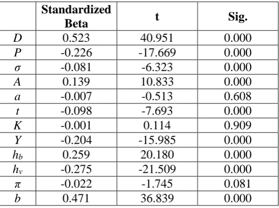
In a second step, we analysed the influence of the problem parameters on the relative advantage of the two delivery structures proposed in this paper. For this purpose, we conducted a regres-sion analysis between the problem parameters and the ratio of the expected total costs of both structures as given by the quotient of (7) and (11). The results of the regression analysis with the problem parameters as independent variables and the ratio of the expected total costs as the dependent variable are given in Table 5. As can be seen, a statistically relevant relationship (with Sig. < 0.05) could be found between all problem parameters and the ratio of the expected total costs, with the exception of K, a and π.
--- Table 5 ---
The results may be interpreted as follows: A higher demand rate or a lower production rate leads to a higher value for the ratio of (7) to (11) and consequently lower relative expected total costs for the case of sequential deliveries. This may be explained by the fact that both an in-crease in D and a decrease in P, ceteris paribus, lead to a higher value of nmin, i.e. a higher
minimum number of suppliers the buyer needs to contract. In case the suppliers deliver sequen-tially to the buyer, an increase in the number of suppliers reduces inventory carrying costs both at the buyer and at the suppliers, whereas in case of simultaneous deliveries, inventory is only reduced at the suppliers. As a consequence, a higher value for nmin results in an increase in the
supplier handling costs for both delivery structures, but in a higher reduction in inventory in case suppliers deliver sequentially. This explains why the relative advantage of model SEQ increases in nmin.
12 deliveries since simultaneous deliveries lead to scale effects in the receiving department. The ordering costs obviously have an opposite effect.
The impact of hb on the relative advantage of both delivery structures may be explained by the
fact that in case of sequential deliveries, inventory is reduced at the buyer, wherefore this de-livery structure is especially beneficial in case inventory carrying costs at the buyer are high. In contrast, since more suppliers are contracted in case of model SEQ as compared to model SIM, more inventory has to be kept at the suppliers. Consequently, as hv increases, the relative
advantage of model SEQ is reduced.
A last effect that could be identified is that an increase in b increases the relative advantage of model SEQ. This result is caused by the fact that in case of sequential deliveries, the buyer incurs a smaller stockout risk per delivery, but faces this stockout risk more often. Obviously, higher values for b reduce the overall risk stronger in case of model SEQ as compared to model SIM, which necessitates a lower adjustment of the other model parameters and consequently increases the advantage of this delivery structure.
To assess the risk behaviour of both models, we conducted a second regression analysis with the problem parameters as independent variables and the ratio of the backorder quantities as the dependent variable. The results are presented in Table 6.
--- Table 6 ---
The results illustrate that P, Y, hb, hv, π and b had a significant influence on the ratio of the
backorder quantities, while the influence of the other parameters was very small or statistically insignificant. As can be seen, an increase in P leads to a relatively higher amount of backorders in the case of simultaneous deliveries. Again, this may be explained by the influence of P on
nmin, which may reduce the number of suppliers and entail that the buyer incurs a higher
stock-out risk per delivery which he/she faces less often. As indicated above, this may reduce the overall stockout risk.
A second aspect that could be identified is that a reduction in Y leads to a relatively higher amount of backorders in the case of simultaneous deliveries. This may again be explained by the order frequency effect: If Y adopts a high value, the number of suppliers is restricted stronger in model SEQ, which results in higher production quantities, longer lead times and consequently higher backorder quantities. Obviously, this is a result of the scale effects the company realises in model SIM, where deliveries are received at the same time and where the workload in the receiving department can be reduced. The influence of hb and hv may be
ex-plained analogous. An increase in the backorder costs also has a stronger impact on the backorder quantity in the case of sequential deliveries. This is due to the fact that lead time was on average slightly higher in model SEQ than in model SIM, wherefore an increase in π neces-sitated a larger reduction of lead time in this case. Further, backorders occur n times per lot in case of model SEQ, which intensifies this effect. The influence of b on the backorder quantities of both models finally has already been explained above.
Conclusion
13 The contribution of the paper is twofold: First, it extends prior works on integrated inventory models to consider multiple suppliers and the supplier selection decision in a setting with sto-chastic demand and variable lead time, and second it studies how multiple sourcing influences the risk of incurring a stockout in case of a deterministic lead time and stochastic demand. Both aspects have not been analysed in the literature before.
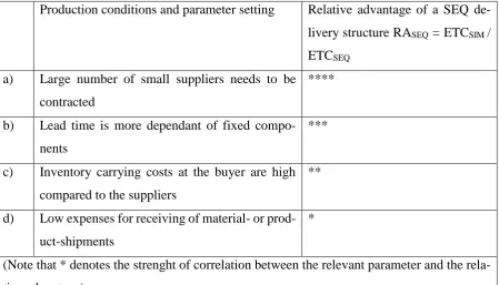
The results of the paper indicate that a delivery structure with sequential deliveries outperforms the case where suppliers deliver simultaneously to the buyer in most cases, although the risk of incurring a stockout is not necessarily lower in case of sequential deliveries. Based on our simulation study, we conclude that sequential deliveries are especially beneficial in case a) the buyer faces small suppliers and consequently needs to receive products from a large number of sources to satisfy demand, b) receiving efforts for the considered products or materials and associated expenditures at the buyer are low, c) fixed lead time components are high as com-pared to order quantity-dependant lead time components and d) inventory carrying costs at the buyer are high whereas inventory carrying costs at the suppliers are low. Table 7 summarises factors that influence the relative advantage of delivery structure SEQ.
--- Table 7 ---
If one or more of these conditions are not met, the relative advantage of sequential deliveries decreases, although this delivery structure may still lead to lower expected total costs than the case of simultaneous deliveries. The question which delivery structure is better in a certain scenario depends on the problem parameters, although we were able to identify cost tendencies. The implications for practitioners clearly are that in case the conditions mentioned above are met, a sequential delivery structure should be implemented to reduce the total costs of ordering and receiving the product. In cases where some or all of these conditions are not met, choosing a delivery structure with simultaneous deliveries results in a lower increase in expected total costs. In addition, if we assume that situations may arise where companies try to minimise the number of shipments they receive, for example because limited resources are available in the receiving area of the company (for further examples, the reader is refereed to Gardner and Dannenbring, 1979; Schneider and Rinks, 1989; Ellram and Siferd, 1993), it may be beneficial to implement simultaneous deliveries. Cases with limited receiving resources may be inter-preted as a restriction on the number of shipments a company is able to receive. In such a situation, a company may search for cost-optimal solutions without investing in new resources. Thus, it may be beneficial to implement a simultaneous delivery strategy with an optimal pa-rameter setting as compared to a sequential strategy with a non-optimal papa-rameter setting caused by this restriction. Further, the costs of receiving shipments may be difficult to estimate in practical situations. In such a case, if the costs of model SIM and model SEQ are close to each other, the company may decide to implement model SIM to reduce work in the receiving department without explicitly estimating receiving costs (which, in turn, may also be associated with costs). We conclude that there are situations where a company may want to implement a SIM policy although it leads to (slightly) higher total costs than model SEQ.
14 influence the question of how many and which suppliers to select. A heuristic method for se-lecting suppliers in an integrated inventory model, which, however, is only applicable to cases where demand is deterministic, can be found in Glock (2011a). Further extensions may include the study of batch shipments, which have also been shown to reduce stockout risk (see e.g. Ben-Daya and Hariga, 2004), or other types of risks, such as uncertain lead times or product quality.
Acknowledgement
The authors are grateful to the anonymous referees for their valuable comments and sugges-tions on an earlier version of this paper.
References
Ben-Daya, M., Darwish, M., Ertogral, K., 2008. The joint economic lot sizing problem: Review and extensions. European Journal of Operational Research, 185, 726-742.
Ben-Daya, M., Hariga, M., 2003. Lead-time reduction in a stochastic inventory system with learning consideration. International Journal of Production Research, 41, 571-579.
Ben-Daya, M., Hariga, M., 2004. Integrated single vendor single buyer model with stochastic demand and variable lead time. International Journal of Production Economics, 92, 75-80. Ben-Daya, M., Raouf, A., 1994. Inventory Models Involving Lead Time as a Decision
Varia-ble. Journal of the Operational Research Society, 45, 579-582.
Cao, M., Vonderembse, M. A., Zhang, Q., Ragu-Nathan, T. S., 2010. Supply chain collabora-tion: conceptualisation and instrument development. International Journal of Production Re-search, 48, 6613-6635.
Chandra, C., Grabis, J., 2008. Inventory management with variable lead-time dependent pro-curement cost. Omega, 36, 877-887.
Chiang, C., Benton, W. C., 1994. Sole Sourcing versus Dual Sourcing under Stochastic De-mands and Lead Times. Naval Research Logistics, 41, 609-624.
Chopra, S., Meindl, P., 2007. Supply Chain Management. 3rd ed. Upper Saddle River: Pearson Prentice Hall.
Ellram, L.-M., Siferd, S.P., 1993. Purchasing: The cornerstone of the total cost of ownership concept. Journal of Business Logistics,14, 163-184.
Ganeshan, R., 1999. Managing supply chain inventories: A multiple retailer, one warehouse, multiple supplier model. International Journal of Production Economics, 59, 341-354. Ganeshan, R., Tyworth, J.E., Guo, Y., 1999. Dual sourced supply chains: the discount supplier
option. Transportation Research Part E, 35, 11-23.
Gardner, E.S., Dannenbring, D.G., 1979. Using optimal policy surfaces to analyze aggregate inventory tradeoffs. Management Science,25, 709-720.
Glock, C.H., 2009. A Comment: “Integrated single vendor single buyer model with stochastic demand and variable lead time”. International Journal of Production Economics, 122, 790-792.
Glock, C.H., 2011a. A multiple-vendor single-buyer integrated inventory model with a variable number of vendors. Computers & Industrial Engineering, 60, 173-182.
Glock, C.H., 2011b. A comparison of alternative delivery structures in a dual sourcing envi-ronment. International Journal of Production research, DOI: 10.1080/00207543.2011.592160.
Glock, C.H., In Press a. Lead time reduction strategies in a single-vendor-single-buyer inte-grated inventory model with lot size-dependent lead times and stochastic demand. Interna-tional Journal of Production Economics, DOI: 10.1016/j.ijpe.2011.09.007.
15 Goyal, S.K, Gupta, Y.P., 1989. Integrated inventory models: The buyer-vendor coordination.
European Journal of Operational Research, 41, 261-269.
Hadley, G., Whitin, T.M., 1963. Analysis of Inventory Systems. Prentice-Hall, Englewood Cliffs, NJ.
Hayya, J.C., Christy, D.P., Pan, A., 1987. Reducing inventory uncertainty: a reorder point sys-tem with two vendors. Production and Inventory Management, 28, 43-48.
Hendricks, K. B., Singhal, V. R., 2005a. An Empirical Analysis of the Effect of Supply Chain Disruptions on Long-Run Stock Price Performance and Equity Risk of the Firm. Production and Operations Management, 14, 35-52.
Hendricks, K.B., Singhal, V. R., 2005b. Association Between Supply Chain Glitches and Op-erating Performance. Management Science, 51, 695-711.
Hill, R.M., 1996. Order splitting in continuous review (Q,r) inventory models. European Jour-nal of OperatioJour-nal Research, 95, 53-61.
Hillier, F.S., Lieberman, G.J., 2001. Introduction to Operations Research, McGraw-Hill, Bos-ton, MA.
Hsiao, Y.-C., 2008.Integrated logistic and inventory model for two-stage supply chain con-trolled by the reorder and shipping points with sharing information. International Journal of Production Economics. 115, 229-235.
Jha, J.K., Shanker, K., 2009. A single-vendor single-buyer production-inventory model with controllable lead time and service level constraint for decaying items. International Journal of Production Research, 47, 6875-6898.
Kelle, P., Miller, P.A., 2001. Stockout risk and order splitting. International Journal of Produc-tion Economics, 71, 407-415.
Kelle. P., Miller, P.A., Akbulut, A.Y., 2007. Coordinating ordering/shipment policy for buyer and supplier: Numerical and empirical analysis of influencing factors. International Journal of Production Economics, 108, 100-110.
Kelle, P., Silver, E.A., 1990a. Decreasing expected shortages through order splitting. Engineer-ing Costs and Production Economics, 19, 351-357.
Kelle, P., Silver, E.A., 1990b. Safety Stock Reduction by Order Splitting. Naval Research Lo-gistics, 37, 725-743.
Kheljani, J.G., Ghodsypour, S.H., O’Brien, C., 2009. Optimizing whole supply chain benefit versus buyer’s benefit through supplier selection. International Journal of Production Eco-nomics, 121, 482-493.
Kim, J.S., Benton, W.C., 1995. Lot size dependent lead times in a Q,R inventory system. In-ternational Journal of Production Research, 33, 41-58.
Kim, T., Goyal, S.K., 2009. A consolidated delivery policy of multiple suppliers for a single buyer. International Journal of Procurement Management, 2, 267-287.
Lau, H.-S., Zhao, L.-G., 1993. Optimal ordering policies with two suppliers when lead times and demands are all stochastic. European Journal of Operational Research, 68, 120-133. Liao, C.J., Shyu, C.H., 1991. An Analytical Determination of Lead Time with Normal Demand.
International Journal of Operations and Production Management, 11, 72-78.
Norman, A., Jansson, U., 2004. Ericsson’s proactive supply chain risk management approach after a serious sub-supplier accident. International Journal of Physical Distribution and Lo-gistics Management, 34, 434-456.
Oladi, R., Gilbert, J., 2009. Buyer and Seller Concentration in Global Commodity Markets. Working Paper, Utah State University.
16 Ouyang, L.-Y., Yeh, N.-C., Wu, K.-S., 1996. Mixture Inventory Models with Backorders and Lost Sales for Variable Lead Time. Journal of the Operational Research Society, 47, 829-832.
Pan, J.C.H., Lo, M.C., 2008. The learning effect on setup cost reduction for mixture inventory models with variable lead time. Asia-Pacific Journal of Operational Research, 25, 513-529. Park, S.S., Kim, T., Hong, Y., 2006. Production allocation and shipment policies in a
multiple-manufacturer-single-retailer supply chain. International Journal of Systems Science, 37, 163-171.
Ramasesh, R.V., Ord, J.K., Hayya, J.C., Pan, A., 1991. Sole versus dual sourcing in stochastic lead-time (s,Q) inventory models. Management Science, 37, 428-443.
Ramasesh, R.V., Ord, J.K., Hayya, J.C., 1993. Note: Dual Sourcing with Nonidentical Suppli-ers. Naval Research Logistics, 40, 279-288.
Rosenblatt, M.J., Herer, Y.T., Hefter, I., 1998. Note. An Acquisition Policy for a Single Item Multi-Supplier System. Management Science, 44, S96-S100.
Ryu, S.W., Lee, K.K., 2003. A stochastic inventory model of dual sourced supply chains with lead-time reduction. International Journal of Production Economics, 81-82, 513-524. Sajadieh, M.S., Eshghi, K., 2009. Sole versus dual sourcing under order dependent lead times
and prices. Computers and Operations Research, 36, 3272-3280.
Schneider, H., Rinks, D.B., 1989. Optimal policy surfaces for a multi-item inventory problem. European Journal of Operational Research, 39, 180-191.
Sculli, D., Wu, S.Y., 1981. Stock Control with Two Suppliers and Normal Lead Times. Journal of the Operational Research Society, 32, 1003-1009.
Sculli, D., Shum, Y.W., 1990. Analysis of a Continuous Review Stock-control Model with Multiple Suppliers. Journal of the Operational Research Society, 41, 873-877.
Smith, H.; Thanassoulis, J., 2008. Upstream Competition and Downstream Buyer Power. Eco-nomic Series Working Paper Nr. 420, University of Oxford.
Tang, C.S., 2006. Perspectives in supply chain risk management. International Journal of Pro-duction Economics, 103, 451-488.
Thomas, D.J., Tyworth, J.E., 2006. Pooling lead-time risk by order splitting: A critical review. Transportation Research E: Logistics and Transportation Review, 42, 245-257.
Zequeira, R., Durán, A., Gutiérrez, G., 2005. A mixed inventory model with variable lead time and random back-order rate. International Journal of Systems Science, 36, 329-339.
Table Captions
Table 1: Sample data set
Table 2: Results for the sample data set
Table 3: Parameter ranges employed in the generation of the random data sets Table 4: Illustration of the relative advantage of model SIM and model SEQ Table 5: Results of the regression analysis for the ratio of the expected total costs Table 6: Results of the regression analysis for the ratio of the backorder quantities Table 7: Factors that influence the relative advantage of delivery structure SEQ
Figures Captions
Figure 1: Alternative delivery structures for a system with two suppliers and a single buyer
Tables and Figures
17
D = 150 demand rate in units per unit time
P = 160 production rate in units per unit time
σ = 10 standard deviation of demand
A = 75 ordering costs per order
a = 8 first cost parameter of the supplier handling cost function
t = 1.75 second cost parameter of the supplier handling cost function
Y = 150 receiving costs per delivery
K = 300 setup and transportation costs per production lot at the supplier
hb = 6 unit inventory carrying charges per unit of time at the buyer
hv = 3 unit inventory carrying charges per unit of time at the vendors
π = 100 backorder costs per unit backordered
[image:18.595.53.551.399.763.2]b = 0.1 fixed delay factor
Table 1: Sample data set.
Effects of the key model parameters
Simultaneous Deliveries Sequential Deliveries
Q n SS SL ETC Q n SS SL ETC
D 150 183 2 12 92.68 1469.32 505 4 15 94.95 1256.56
250 223 2 14 94.65 1994.33 593 4 18 96.44 1754.66
350 315 3 14 94.60 2706.26 649 4 20 97.22 2224.60
P 160 183 2 12 92.68 1469.32 505 4 15 94.95 1256.56
260 141 1 13 94.36 1208.79 542 4 13 94.58 1163.66
360 146 1 11 94.16 1162.05 562 4 11 94.38 1118.50
σ 5 185 2 6 92.60 1422.59 511 4 8 94.89 1198.25 10 183 2 12 92.68 1469.32 505 4 15 94.95 1256.56
20 181 2 24 92.76 1562.59 493 4 31 95.07 1372.67
A 50 181 2 12 92.76 1448.71 376 3 15 94.99 1248.84
75 183 2 12 92.68 1469.32 505 4 15 94.95 1256.56
100 186 2 12 92.56 1489.61 634 5 15 94.93 1262.93
a 4 182 2 12 92.72 1458.26 746 6 15 95.03 1240.35
8 183 2 12 92.68 1469.32 505 4 15 94.95 1256.56
12 185 2 12 92.60 1480.28 383 3 15 94.89 1269.54
t 1.5 183 2 12 92.68 1465.81 875 7 15 95.00 1245.22
18 2 184 2 12 92.64 1473.47 382 3 15 94.91 1265.59
Y 100 178 2 12 92.88 1427.79 478 4 15 95.22 1195.51
150 183 2 12 92.68 1469.32 505 4 15 94.95 1256.56
200 189 2 12 92.44 1509.62 530 4 16 94.70 1314.53
K 200 160 2 12 93.60 1294.64 449 4 15 95.51 1130.80
300 183 2 12 92.68 1469.32 505 4 15 94.95 1256.56
400 240 1 17 90.40 1587.78 555 4 16 94.45 1369.81
hb 4 215 2 14 94.27 1245.98 575 4 18 96.17 1089.18
6 183 2 12 92.68 1469.32 505 4 15 94.95 1256.56
8 163 2 11 91.31 1664.26 456 4 14 93.92 1405.62
hv 1 240 1 17 90.40 1300.28 567 4 16 94.33 1131.40
3 183 2 12 92.68 1469.32 505 4 15 94.95 1256.56
5 173 2 12 93.08 1552.74 460 4 15 95.40 1369.32
π 50 185 2 9 85.20 1452.96 510 4 12 89.80 1239.08 100 183 2 12 92.68 1469.32 505 4 15 94.95 1256.56
150 183 2 14 95.12 1477.90 502 4 17 96.65 1265.86
b 0.01 131 1 15 94.76 1299.12 503 4 15 94.97 1250.50
[image:19.595.76.261.544.755.2]0.10 183 2 12 92.68 1469.32 505 4 15 94.95 1256.56 1.00 283 2 17 88.68 1639.18 516 4 22 98.84 1305.04
Table 2: Results for the sample data set.
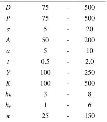
Parameter ranges for simulation
D 75 - 500
P 75 - 500
σ 5 - 20
A 50 - 200
a 5 - 10
t 0.5 - 2.0
Y 100 - 250
K 100 - 500
hb 3 - 8
hv 1 - 6
19
b 0.01 - 1.00
Table 3: Parameter ranges employed in the generation of the random data sets.
Example 1 a A b D hb hv K P π
7.66 151.31 0.29 427.96 3.93 5.67 131.00 146.41 86.56
Example 2 a A b D hb hv K P π
8.10 70.61 0.05 233.90 7.84 3.24 459.40 355.83 115.01
σ t Y ETC SIM ETC SEQ
14.95 1.37 219.47 2720.13 2749.43
σ t Y ETC SIM ETC SEQ
[image:20.595.76.457.192.366.2]11.70 1.50 185.51 1977.56 1915.23
Table 4: Illustration of the relative advantage of model SIM and model SEQ.
Standardized
Beta t Sig.
D 0.523 40.951 0.000
P -0.226 -17.669 0.000
σ -0.081 -6.323 0.000
A 0.139 10.833 0.000
a -0.007 -0.513 0.608
t -0.098 -7.693 0.000
K -0.001 0.114 0.909
Y -0.204 -15.985 0.000
hb 0.259 20.180 0.000
hv -0.275 -21.509 0.000
π -0.022 -1.745 0.081
[image:20.595.73.347.424.628.2]b 0.471 36.839 0.000
Table 5: Results of the regression analysis for the ratio of the expected total costs.
Standardized
20
D -0.031 -1.505 -0.132
P 0.098 4.759 0.000
σ -0.009 4.759 0.680
A 0.043 2.086 0.037
a 0.034 1.631 0.103
t -0.051 -2.450 0.014
K 0.045 2.189 0.029
Y -0.161 -7.085 0.000
hb 0.103 4.960 0.000
hv 0.154 7.456 0.000
π -0.228 -10.998 0.000
[image:21.595.73.347.72.245.2]b 0.494 23.894 0.000
Table 6: Results of the regression analysis for the ratio of the backorder quantities.
Production conditions and parameter setting Relative advantage of a SEQ
de-livery structure RASEQ = ETCSIM /
ETCSEQ
a) Large number of small suppliers needs to be
contracted
****
b) Lead time is more dependant of fixed
compo-nents
***
c) Inventory carrying costs at the buyer are high
compared to the suppliers
**
d) Low expenses for receiving of material- or
prod-uct-shipments
*
(Note that * denotes the strenght of correlation between the relevant parameter and the
rela-tive advantage)
[image:21.595.75.525.326.583.2]