HIGH RESOLUTION MODELLING FOR PERFORMANCE ASSESSMENT OF
FUTURE DWELLINGS
Jon Hand, Nick Kelly, Aizaz Samuel
Energy Systems Research Unit, University Of Strathclyde, Glasgow, Scotland, UK
ABSTRACT
In future low-energy buildings, electrical power and hot water use will feature prominently in the overall energy demand. Unlike space heating, these demand constituents are intermittent and vary rapidly over a few seconds. However, most building simulation tools operate at a longer time resolutions, utilising hourly climate data and so may be unable to properly capture the electrical or hot water demand characteristics. This paper demonstrates means by which electrical demand/generation and hot water draws can be modelled at higher time resolutions (1-minute) than is usually done at present. An approach to generating high-resolution climate data is also presented. An illustrative simulation highlighted different outcomes when modelling future buildings at low and high time resolutions. This showed that (in this case) although the overall energy demands and yields were similar, there discrepancies between the two temporal resolutions for import, export and self-consumption of electricity of up to 25%.
INTRODUCTION
A combination of improved fabric insulation and air tightness is likely to reduce the primacy of space heating demands and place more of a focus on electrical demands and hot water use in future dwellings. For example in a typical UK house, space heating accounts for around 65% of its total energy demand (Palmer and Cooper, 2012); in a Passive House, space heating can account for as little as 40% of the dwelling’s energy demand (Feist, 2006). Housing stock improvements are already beginning to have an effect in this picture. For example, in the UK as a whole, total household space heating energy demand has declined by 21% since 2004; conversely, total household energy demand associated with electrical appliance use has climbed approximately 15% over the same period (Palmer and Cooper, 2012). Hot water use is also an important component of domestic energy consumption accounting for around 17% of total UK household energy use (Palmer and Cooper, 2012).
In parallel with changing energy end use characteristics, the supply of energy to dwellings is
also undergoing a significant transformation through the supply of electrical energy from local low-carbon sources. For example, in the UK, over 2GW of microgeneration capacity has been installed since the introduction of a feed-in-tariff in 2010, the vast bulk of this capacity takes the form of domestic photovoltaic (PV) arrays (OFGEM, 2013).
Temporal Characteristics of PV Output and Hot Water and Electrical Demand
Hot water and electrical demand, along with electrical supply from PV share similar characteristics in that they exhibit rapid changes in magnitude over short time periods. For example, the output from a PV array will diminish significantly in proportion to the available solar radiation over the period of a few seconds as clouds pass over the sun: a situation that occurs all too frequently in the UK’s maritime climate. Figure 1 shows the variability of solar radiation in partially cloudy conditions. Figures 2 and 3 illustrate the variability of electrical demand and hot water demand, respectively. By contrast, space heating tends to vary gradually and over longer time scales (up to an hour) due to the influence of a building’s intrinsic thermal mass.
Higher Resolution in Building Simulation
Given the temporal characteristics of the energy flows highlighted, a recurring message in the literature is that time resolutions of as low as 1-minute are required to adequately capture the characteristics of electrical demand and supply and the use of hot water.
Figure 1 rapid variability seen in (5-min) monitored solar insolation.
Figure 2 monitored (5-min) electrical demand on a UK family dwelling (IEA ECBCS Annex 42, 2007).
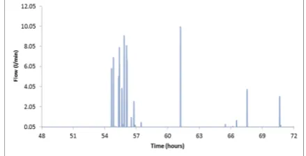
Figure 3 hot water draws monitored (at 10-min intervals) in a UK family dwelling.
Jordan and Vagen (2005) in IEA SHC Task 26 specify a 1-minute resolution to produce domestic hot water (DHW) draws; IEA ECBS Annex 42 adopted the same approach. Renné et al (2008) indicated that solar data with a time resolution of 15 minutes or less is required when assessing the interaction of PV with power networks and for economic modelling. Hawkes and Leach (2005) looked at the temporal resolution of modelling required to properly assess the economics of microgeneration (for the related case of domestic micro-combined heat and power [µCHP]), specifically looking at revenue from electricity export and self-consumption (i.e. locally generated electricity used within the building). They indicated that time steps of 10-minutes or less were required in order to capture the variation in the export and import of electricity to and from electricity network, respectively, and provide an accurate assessment of potential income. Whilst most simulation tools can operate at sub-hourly time-intervals, most produce hourly calculations as a default, as they utilise readily available hourly climate data as a boundary condition for the solution of their underpinning energy equations. A quick review of papers published in IBPSA conferences (IBPSA, 2014) indicates that many tool users utilise the default time resolution in modelling studies.
Aim
As electrical import and export, and hot water demand become more prominent in future buildings, this paper explores whether modelling these boundary conditions at a higher resolution could have a substantial impact on building energy performance predictions. Specifically, this paper looks at the provision of high-resolution data to characterise electrical demands, hot water use and solar irradiation. Further, by way of illustration, the results from a high-resolution simulation of a case study ‘zero-energy’ building are compared to those from an hourly simulation.
Previous Work on High Resolution Modelling There are a range of papers in the literature specifically looking at the provision of high resolution solar data. For example, Janak (1997) and Walkenhorst et al (2002) employ the Skartveit and Olseth model (1992) (or variants) to generate 1-min stochastic solar data from hourly means. More recently, Richardson et al (2011) and McCracken (2011) used a customised 1st order Markov chain, with its transition probabilities derived from a base sample of real high resolution data, to generate various stochastic sub-hourly solar datasets.
There have been several efforts to generate high-resolution electrical demand data for building simulation and a variety of other uses. Capasso et al (1994) used time use survey data and a ‘bottom-up’ (appliance level) approach to generate stochastic domestic electrical demand profiles at 15-minute resolution. Stokes et al (2005), Widen and Wackelgard (2010) and Richardson et al (2010) also used time-use survey data and a bottom-up approach to generate 1-minute resolution appliance electrical demand data. Borg and Kelly (2011) used an Italian appliance usage dataset coupled with a data from the UK on prospective improvements in appliance energy efficiency to generate high-resolution electrical demand profiles for future dwellings. Some key work on high resolution hot water demand modelling was that undertaken by Jordan and Vagen (2005), who developed a stochastic modelling approach to generate hot water demand profiles at a 1-minute time resolution. The authors determined that the use of higher resolution demand profiled led to significant changes in the predicted stratification characteristics of a solar domestic hot water storage tanks compared to the use of more simplistic hourly draw profiles, though the impact on energy performance seemed to be small.
MODELLING APPROACH
[image:2.595.68.290.67.428.2]simulated at different time resolutions and the results analysed.
High Resolution Electrical Demand
For this paper, the work of Richardson et. al. (2010) has been adapted to enable the generation of complementary appliance heat gains profiles. Richardson et. al. employ a bottom-up approach to electrical demand profile generation: on a time step-by-time step basis, the probability that an appliance will be active is tested against a randomly generated number between 0 and 1. If then the appliance is deemed to be on ( 1 at some time , otherwise it is deemed to be off ( 0). The probability is derived from time-use survey data and is related to the number of occupants active in a dwelling. The approach can be employed for a population of appliances (and lighting) to generate a whole-dwelling demand profile at high resolution. For this paper, the calculation approach defined by Richardson et. al.
has been expanded such that 1) heat gains from electrical appliances can be generated and 2) the heat gains can be spatially distributed. To calculate the heat gain, the assumption is that first, that a user-defined fraction () of a device’s electrical consumption is ultimately dissipated as heat; and secondly that each appliance has a location in the building (corresponding to a thermal zone in a simulation model). The resulting heat gain from a group of appliances at location will therefore be:
∑
;
(1)
where n is the total number of appliances and is the nominal power consumption (W) of appliance j. Note that this approach implicitly assumes that the heat gain is instantaneous and secondly that the gain is convective. Both of these assumptions need to be refined in future work.
[image:3.595.306.526.564.676.2]The high-resolution electrical demand data is used with the simulation that follows to help calculate the dwelling’s electrical power flows, specifically the import/export of power. The corresponding heat gain profiles (which also include heat gains from occupants) are used in the calculation of the dwelling’s thermal performance.
Figure 4 stochastically generated electrical demand and corresponding heat gain profiles.
High Resolution Hot Water Demand
A model of domestic hot water draws has been developed for the ESP-r tool, based on the work of Jordan and Vagen (2005). At each simulation time step the model calculates if a hot water draw occurs for a variety of user-defined draw ‘types’. The draw types defined could be baths, showers, washing appliances and domestic sinks. The user also defines when the draws nominally occur during the day, by defining the typical percentage of the daily water demand consumed within contiguous user-defined periods such as morning, afternoon, evening, etc. At each simulation time step, the probability of a hot water draw occurring for a specific type i, at some time t is tested by comparing a random number ρ (generated each time step) to a probability threshold calculated using the following equation.
!"∆$
%
∆$∆$
;
(2)
where & is the nominal daily hot water draw (l) for the household, and ' are the fractions of the daily draw taken by the draw type and taken during time period S, respectively; ()* is the nominal draw flow rate (l/s) for type i and ∆ is the draw duration (s). Finally, ∆ is the simulation time step (s) and ∆' is the duration of the period S (s). If + then the draw takes place.
The specific draw flow rate is derived from a normal distribution characterised by a mean draw flow rate, ,̅ (l/s) and a standard deviation .. Should a draw for a specific type occur, then the draw flow rate ( (l/s) is determined by comparing a second random number / against the cumulative probability for the flow rate of the hot water draw type 0(1 in the range ,̅ 2 π.4 (14 ,̅ 5 π.. So, when / ≃ 0(1; then ( (1. A typical output is shown in figure 5. In the simulation that follows, the high-resolution hot water demand calculation is a boundary condition linked in to the model of the dwelling’s heating system.
Figure 5 stochastically-generated hot water demand.
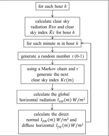
High Resolution Solar Data
[image:3.595.72.285.623.708.2]60 stochastic values generated using a 1st-order Markov chain. The process, shown in Figure 4, calculates 60 global horizontal radiation values for each hour (W/m2); these are then separated into direct normal and diffuse horizontal values using the approach developed by Louche et al (1991).
Figure 6 generating 1-minute-resolution solar data.
[image:4.595.315.522.583.746.2]The Markov chain was calibrated using real, high-resolution data from Reading; McCracken (2011) demonstrated that the resulting transition probability matrix (TPM) could be used to generate representative solar data for disparate UK geographical locations (using the local hourly data as the basis for the calculation). The work hinted that whilst the occurrence of different solar conditions may be differ widely in different geographical locations, the probability of transitioning from one solar state to another may be geographically insensitive (this hypothesis, however, remains to be fully tested). Figure 7 shows sample hourly and 1-minutely data generated using the approach described.
Figure 7 Sample of hourly and stochastic 1-minute resolution solar data.
CASE STUDY: ‘ZERO ENERGY’ HOUSE
An ESP-r model of a hypothetical ‘zero-energy’ house was used to explore the impact of simulating performance at a higher time resolution. The simulation was run over a calendar year at 1-minute and 1-hour resolutions. To ensure consistency for the purposes of comparison, the 1-hour time resolution simulations use hourly-averaged boundary conditions derived from the 1-minute simulation. The model used a climate dataset from Southern England, which was geographically compatible with the Reading data used as the basis for the generation of the 1-minute resolution stochastic solar data.The floor areas and volumes used in the model are characteristic of ‘typical’ UK housing and were selected following reviews of housing stock characteristics undertaken for a previous projects (e.g. Kelly and Beyer, 2008).
Table 1 general geometric characteristics.
Floor area (m2) 82.7
External surface area (m2) 151
Occupied Volume (m3) 230
Glazed Area (m2) 21.45
‘Day’ zone floor area (m2) 34.8
‘Night’ zone floor area (m2) 47.9
[image:4.595.72.289.601.710.2]The model features a mono pitch roof to accommodate the 45m2 (8 kWp) of PV panels required to offset the electrical demand (see figure 6). The model is divided into three main thermal zones: a loft zone and two composite zones describing (respectively) the areas of the dwelling hosting active occupancy such as the living room and kitchen and those areas that have low occupancy rates or that are occupied at night such as bathrooms and bedrooms, respectively. This geometrically aggregated form of the model captures the pertinent thermodynamic characteristics of the building’s performance and has been deployed successfully in other studies, e.g. (Clarke et al, 2008).
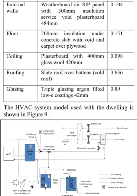
The building meets passive house standards, being super-insulated, with a wooden frame construction, triple-glazed windows and with high airtightness. The characteristics of the key fabric elements (constructions) are as shown in Table 3.
Table 2 characteristics of constructions used in the dwelling model.
Construction Details U-value (W/m2K)
External walls
Weatherboard air SIP panel with 300mm insulation service void plasterboard 484mm
0.104
Floor 200mm insulation under concrete slab with void and carpet over plywood
0.151
Ceiling Plasterboard with 400mm glass wool 420mm
0.098
Roofing Slate roof over battens (cold roof)
3.636
Glazing Triple glazing argon filled low-e coatings 42mm
0.89
[image:5.595.65.292.183.508.2]The HVAC system model used with the dwelling is shown in Figure 9.
Figure 9 systems model for the dwelling.
Heat distribution is convective, via the mechanical ventilation heat recovery system (MVHR) shown above, and the heat source is an air source heat pump (ASHP) with a 6kW capacity and nominal COP of 3; this is used in conjunction with a 500L thermal buffer, which allows the heat pump to be operated flexibly in time. The heat pump charges the thermal buffer, which then supplies the heat for space heating and hot water. The system also includes a dedicated 500L solar domestic hot water tank and 3m2 of roof-mounted solar collectors. Another feature of the model is a grey-water-heat-recovery-system (GWHR): this collects wastewater from the baths, showers, etc. in a 200L tank, which pre-heats the incoming cold-feed to the hot water tank via a heat exchanger.
Finally, the model features a basic electrical network, representing the house’s distribution system and to which the PV and all power consuming equipment are connected. The electrical network includes a
connection to the electricity network and is used here to track the electrical supply and demand, the electrical import export with the wider grid and the electrical losses including the inverter and cable losses.
RESULTS AND DISCUSSION
The ESP-r simulations of the dwelling produce time-series data of the building’s temperatures and heat and mass flows and the electrical power flows; these have been post-processed and aggregated in order to generate the performance metrics shown in the tables that follow. Three specific areas of performance are analysed in order to assess the impact of the change in the temporal resolution of the boundary conditions. These are: 1) electrical energy balance; 2) hot water and solar domestic hot water performance; and 3) the ASHP performance.
Electrical Energy Balance
The electrical energy balance of the dwelling is directly affected by the high-resolution solar data and the use of high-resolution electrical demand data, the use of both changes the temporal characteristics of the supply-demand match. Table 3 shows the electrical output from both the 1-hour and 1-minute time resolution simulations over a 12-month period.
Figure 10 PV generation and demand for electricity – September day at 1-hour and 1-minute resolution.
Table 3 indicates that the annual PV-generation differs by around 3.5%, with the hourly data consistently giving lower output. The reason for this difference lies in ESP-r’s PV model; this calculates power output as a non-linear function of incident solar radiation and PV temperature. Higher insolation levels producw disproportionately higher power output compared to lower solar insolation at the same PV panel temperature. So, hourly-averaged solar data produces a slightly lower PV yield than when higher resolution data is used (Kelly, 1998).
ASHP
Buffer Tank
+
T
T T
Hot Water
Cold Water Feed Living Space
Temperature
Hot Water Priority Valve Hot Water
Pump
Flow diverting valve Supply fan
Extract fan
Heat
exchanger Air heating coil
Drain
Grey water heat recovery
tank
From house
To house
DHW tank
Roof mounted solar thermal collectors
T
T
outside air
T
hot water piping control wiring temperature sensor
air ducting
[image:5.595.66.293.379.513.2] [image:5.595.309.518.381.607.2]Table 3 Electrical output from the 1-hour and 1-min simulations
*includes inverter and cable losses.
Whilst the net demand and generation figures are broadly similar at both simulation resolutions, the import/export and particularly the self-consumption figures differ significantly. Taking the 1-minute data as the baseline, the hourly simulation electrical annual import value is 10% smaller. The hourly simulation annual export value is 14% smaller and the hourly simulation self-consumption total is 24% larger. The same trend is evident in each month of the simulations. The principal reason for this is illustrated in Figure 10, which shows a typical transition day. The overlap between the PV generation and demand in the hourly data is significantly greater than the overlap in the higher resolution data. Consequently, the hourly data predicts greater self-consumption but less import and export of power.
Hot Water and Solar Performance
The impact of the higher-resolution hot water draws is seen in the hot water tank outlet temperatures shown in Table 4. The hot water energy use and tank losses in both cases was almost identical, varying by less than 0.5%. Similarly, the mean temperature at which hot water is supplied differed by less than 0.2%. The output from the solar thermal collectors differs by 3%, with the hourly simulation predicting slightly less solar output.
Table 4 annual hot water data at different temporal resolutions.
1-hour 1-min
Hot water energy use (kWh) 670 667
Hot water tank losses (kWh) 254 251
Mean hot water draw temp. (oC) 50.7 50.8
Solar thermal output (kWh) 57 59
Figure 11 shows the variation in tank temperature output from the hourly and 1-minute resolution simulations
Figure 11 hot water tank performance over 3-days in September at 1-hour and 1-minute resolution
The variation in tank temperature is very similar though there are some slight temporal variations, particularly in the supply of heat from the heat pump (which is controlled using on/off control with a hot water dead band temperature of 45-55oC). The mass of the large DHW tank damps out the influence of the higher resolution draws.
It should be noted that whilst the thermal results here show that the high resolution hot water draws make little difference, this may not be the case where there is less water storage capacity, e.g. in systems featuring instantaneous hot water heating.
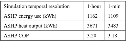
ASHP Performance
Table 5 shows the characteristics of the energy used by and supplied from the heat pump over the course of a year. This shows that the overall electrical energy demand of the heat pump and its heat output vary by less approximately 5% between the two time resolutions. The coefficient of performance differs by less than 1%.
1-Minute Simulations Jan Feb March April May Jun July Aug Sept Oct Nov Dec Annual
Demand kWh 634 572 611 565 514 513 555 500 517 566 553 576 6676
Generation kWh 108 210 484 737 1028 1060 1008 865 591 301 168 83 6643
Import kWh* 578 492 439 357 292 263 281 309 349 465 479 535 4838
Export kWh 53 130 312 530 806 809 734 674 424 201 95 43 4812
Self-con kWh 55 80 172 208 222 250 274 191 167 100 73 40 1831
Hourly simulations Jan Feb March April May Jun July Aug Sept Oct Nov Dec Annual
Demand kWh 634 572 611 565 514 513 555 500 517 566 553 576 6676
Generation kWh 104 202 468 710 989 1024 972 833 570 293 163 80 6407
Import kWh* 548 456 389 309 245 204 225 260 304 432 450 516 4338
Export kWh 28 95 253 454 722 722 645 596 360 162 65 27 4130
Table 5 ASHP performance at different temporal resolutions.
Simulation temporal resolution 1-hour 1-min
ASHP energy use (kWh) 1162 1109
ASHP heat output (kWh) 3671 3483
ASHP COP 3.20 3.18
CONCLUSIONS
This paper focused on high resolution modelling of low-carbon dwellings. Firstly, the means to provide high resolution boundary conditions were discussed, specifically 1-minute resolution stochastic electrical demand data, 1-minute resolution stochastic solar data and 1-minute resolution stochastic hot water draws. Secondly, in order to illustrate the differences between high and low temporal resolution simulation outputs, a model of a hypothetical ‘zero-energy’ dwelling was presented featuring a PV array, ASHP, MVHR and grey water heat recovery. The model performance was simulated over each month of a year at both 1-minute and 1-hour time resolutions. A comparison of the simulation results indicated in terms of gross electrical energy supply and demand that both models produced broadly similar results. However, probing deeper into the output indicated that significant differences, particularly in electrical import, export and self-consumption: with a significantly lower prediction of self-consumption from the 1-minute simulation.
It should be noted that the simulation presented here highlights the potential differences in modelling results (particularly electrical) at different resolutions. However, further modelling work looking at different building types, systems and time resolutions is required to confirm if the differences in predictions highlighted emerge consistently between different time resolution simulations and also to eliminate differences introduced by the stochastic nature of much of the data used.
Analysis of the hot water tank temperature profile and hot water supply temperatures indicated that the use of the high resolution hot water draw data made little difference to the performance predictions, with the 500L tank used in these simulation tending to damp out the influence of the higher resolution draws.
The thermal performance of the heat pump was little influenced by the high-resolution boundary conditions, with the buffering and hot water tank damping out the influence of the higher resolution boundary conditions.
Further work is needed to assess the potential impact of high resolution modelling on systems with less thermal capacitance.
The main finding from the simulations is that in terms of gross energy demands and yields, low and high resolution modelling yield similar results.
However, when assessing the electrical performance of the model and specifically the interaction of the building with the electrical network, the two different resolutions of simulation provided very different results: the high resolution simulation indicated significantly more import and export of power and far less self-consumption of electricity than was evident in the hourly-simulations. Note that whilst the results presented here are not compared to empirical data, the 1-minute electrical boundary data is the more ‘realistic’ in terms of capturing the rapid variability of electrical supply/demand and the related interplay between the house and the electrical network.
FUTURE WORK
The results from the modelling exercise indicate that high-resolution modelling is most applicable in modelling of those systems where electrical power flows are prevalent, e.g. microgeneration, domestic appliance demand. However, the modelling of power flows in these situations needs further refinement. For example, the PV output accounts for inverter losses in a relatively crude fashion with a fixed resistance loss. In reality, the loss is a function of power, moreover the inverter switches on and off as power throughput changed, ‘clipping’ high and low power levels: this feature needs to be properly accounted for in the PV model.
The stochastic calculation electrical demand used in this study uses ‘average’ UK dwelling occupancy statistics; this sometimes produces unrepresentative occupancy profiles with unexpected activity in the middle of the day, work is required to develop more refined and representative taxonomies of occupancy. The heat gain profiles corresponding to the high-resolution appliance demand and occupancy data make crude assumptions regarding the timing (instantaneous heat release) and convective radiant split of the gain (all convective) and should be refined.
Finally, it is worth repeating that the model simulated here is a hypothetical zero-energy dwelling. Consequently, results presented in the paper are specific and intended to be illustrative. More work is required to develop a more general picture of the impact of high resolution modelling on simulation predictions and where it is most appropriately applied.
ACKNOLWEDGEMENTS
The work presented in this paper was undertaken as part of the EPSRC Grand Challenge project: Transformation of the Top and Tail of Energy Networks, funded under EPSRC grant EP/I031707/1.
REFERENCES
Variable Thermal Buffering, Proc. Microgen, National Arts Centre, Ottawa.
Borg S P, Kelly N J, 2011. The effect of appliance energy efficiency improvements on domestic electric loads in European households. Energy and Buildings 43, 2240–2250.
Capasso A, Grattieri W, Lamedica R, & Prudenzi A 1994. A bottom-up approach to residential load modeling. Power Systems, IEEE Transactions on, 9(2), 957-964.
Clarke J A, Johnstone C M, Kim J M and Tuohy P G. Energy 2008. Carbon and Cost Performance of Building Stocks: Upgrade Analysis, Energy Labelling and National Policy Development. Advances. in Building Energy Research. 3: Earthscan: London.
ESRU, 2014. www.esru.strath.ac.uk/Programs/ESP-r.htm Accessed 17 January 2014.
Feist W, 2006. 15th Anniversary of the Darmstadt - Kranichstein Passive House. Available at:
http://www.passivhaustagung.de/Kran/First_Pass ive_House_Kranichstein_en.html Accessed 05 January 2014.
Hawkes, A, Leach, M., 2005. Impacts of temporal precision in optimisation modelling of micro-Combined Heat and Power. Energy 30, 1759– 1779.
IBPSA 2014 http://www.ibpsa.org/?page_id=292
Accessed 16 January 2014.
IEA ECBCS Annex 42, 2007. Datasets. Available from
http://www.ecbcs.org/annexes/annex42.htm
accessed on 5 January 2014.
Janak M 1997. Coupling Building Energy and Lighting Simulation, in Proc. 5th IBPSA World Congress `Building Simulation '97', Prague, Sep 1997, V II, pp313-319, Int. Building Performance Simulation Association, Prague. Jordan U and Vajen K, 2005. DHWCALC: Program
to Generate Domestic Hot Water Draws with Statistical Means for User Defined Conditions, Proc. ISES Solar World Congress, Orlando, US. Kelly N J, Towards a design environment for
building-integrated energy systems: the integration of power flow modelling with building simulation, PhD Thesis, University of Strathclyde, Glasgow.
Knight I and Ribberink H (2007) European and Canadian non-HVAC Electric and DHW Load Profiles for Use in Simulating the Performance
of Residential Cogeneration Systems, IEA ECBCS Annex 42 Report, HMQR, Canada, ISBN 978-0-662-46221-7.
Louche, A., Notton, G., Poggi, P., and Simonnot G. 1991, Correlations for direct normal and global horizontal irradiation. Solar Energy, 46(4) Pg: 261–6.
McCracken D 2011. Synthetic High Resolution Solar Data, MSc Thesis, University of Strathclyde, Glasgow.
OFGEM, 2013. Feed in Tariff Update 14. Available at: https://www.ofgem.gov.uk/publications-and- updates/feed-tariff-update-quarterly-report-issue-14. Accessed on 12 December 2013
Palmer J, Cooper I (eds.), 2012. Great Britain’s Housing Energy Fact File. Department for Energy and Climate Change Publication. URN 12D/354.
Renné D, George R, Wilcox S, Stoffel T, Myers D, and Heimiller D 2008. Solar Resource Assessment, NREL Technical Report NREL/TP-581-42301
Richardson I, Thompson M, Infield D, Clifford C 2010. Domestic electricity use: A high-resolution energy demand model. Eng. and Build. 4210) pp 1878-1887.
Richardson I, Thomson M, 2011. Integrated simulation of photovoltaic micro-generation and domestic electricity demand: a one-minute resolution open-source model, Proc. Microgen II: 2nd International Conference on Microgeneration and Related Technologies, Glasgow.
Skartveit, A., & Olseth, J. A. 1992. The probability density and autocorrelation of short-term global and beam irradiance. Solar Energy, 49(6), 477-487.
Stokes M, 2005. Removing barriers to embedded generation : a fine-grained load model to support low voltage network performance analysis, PhD Thesis, DeMontfort University, Leicester. Walkenhorst, O., Luther, J., Reinhart, C., & Timmer,
J. 2002. Dynamic annual daylight simulations based on one-hour and one-minute means of irradiance data. Solar Energy, 72(5), 385-395. Widén J, Wäckelgård E, 2010. A high-resolution