Workload Ahead Driven Online Energy Minimization Techniques for Battery Powered Embedded Systems with Time Constraints

Minimization Techniques for Battery-Powered

Embedded Systems with Time-Constraints

YUAN CAI University of Iowa

MARCUS T. SCHMITZ Robert Bosch GmbH

BASHIR M. AL-HASHIMI University of Southampton SUDHAKAR M. REDDY University of Iowa

This paper proposes a new online voltage scaling (VS) technique for battery-powered embedded systems with real-time constraints. The VS technique takes into account the execution times and discharge currents of tasks to further reduce the battery charge consumption when compared to the recently reported slack forwarding technique [Ahmed and Chakrabarti 2004], whilst maintain-ing low online complexity ofO(1). Furthermore, we investigate the impact of online rescheduling and remapping on the battery charge consumption for tasks with data dependency which has not been explicitly addressed in the literature and propose a novel rescheduling/remapping technique. Finally, we take leakage power into consideration and extend the proposed online techniques to include adaptive body biasing (ABB) which is used to reduce the leakage power. We demon-strate and compare the efficiency of the presented techniques using seven real-life benchmarks and numerous automatically generated examples.

Categories and Subject Descriptors: J.6 [Computer-aided engineering]: Computer-aided de-sign

General Terms: Design, Algorithms

Additional Key Words and Phrases: Dynamic voltage scaling, Embedded systems, Battery, Adap-tive body biasing

1. INTRODUCTION AND PREVIOUS WORK

Dynamic voltage scaling (DVS) is a powerful technique to reduce the energy con-sumption in embedded computing systems. DVS algorithms can be broadly classi-fied intooffline andonline techniques depending on when the voltage settings are computed. Offline (e.g. [Luo and Jha 2002a], [Andrei et al. 2004], [Schmitz and

Al-Authors’ addresses: Yuan Cai and Sudhakar M. Reddy, Department of Electrical and Computer Engineering, University of Iowa, Iowa City, IA 52242, email: {yucai, reddy}@engineering.uiowa.edu; Bashir M. Al-Hashimi, Department of Electronics and Computer Science, University of Southampton, SO17 1BJ, Southampton, UK, email: [email protected]; Marcus T. Schmitz, Robert Bosch GmbH, Stuttgart D-70442, Germany, email: [email protected];

This work is supported in part by the EPSRC, U.K., under grant GR/S95770

Permission to make digital/hard copy of all or part of this material without fee for personal or classroom use provided that the copies are not made or distributed for profit or commercial advantage, the ACM copyright/server notice, the title of the publication, and its date appear, and notice is given that copying is by permission of the ACM, Inc. To copy otherwise, to republish, to post on servers, or to redistribute to lists requires prior specific permission and/or a fee.

c

Hashimi 2001]) approaches calculate voltage settings, at design time before actual execution, based on worst case execution times (WCET) to guarantee satisfaction of time constraints. Although offline DVS avoids a run-time overhead to compute voltage settings, it fails to exploit online slack arising from tasks executing with less than their WCET (differences>10 times have been reported [Ye and Ernst 1997]). On the contrary, online DVS techniques (e.g. [Aydin et al. 2001], [Pillai and Shin 2001], [Kim et al. 2002], [Luo and Jha 2002b], [Zhu and Mueller 2004]) calculate voltage settings during run-time to utilize such online slack by taking into account the actual execution times (AET) of tasks. Clearly, online techniques have the po-tential to achieve higher energy savings, however, it is necessary to carefully design such online DVS algorithms in order to avoid high run-time overheads that could jeopardize the achievable energy savings and the timing constraints. Many online voltage adjustment approaches for independent tasks have been proposed ([Aydin et al. 2001], [Pillai and Shin 2001], [Kim et al. 2002]). These approaches depend on the schedulability check of the earliest deadline first (EDF) or the rate monotonic (RM) algorithm, which can not be applied to task graphs where there are depen-dent relationships among tasks. The online approach introduced in [Luo and Jha 2002b] calculates the scaling factor for soft aperiodic tasks and considers run-time variations. Zhu and Muller [Zhu and Mueller 2004] utilize a feedback control loop to facilitate DVS and integrated the controller into an earliest deadline first sched-uler. Task scheduling and online voltage scaling are combined in [Zhu et al. 2003]. This work, however, is limited to identical processing element (PE) systems and a straightforward extension toward heterogeneous systems is not apparent. Shin and Kim [Shin and Kim 2001] give a path based intra-task DVS algorithm. The task is modeled as a conditional flow graph in which there is a worst case execution path (WCEP) and an average case execution path (ACEP). Their algorithm inserts voltage scaling points at branch or loop nodes to scale the voltage online based on the ACEP instead of the WCEP. The work in [Shin and Kim 2001] is orthogonal to the proposed algorithm which determines the voltage settings on task-by-task basis (i.e., inter-task voltage scaling). At inter-task level, tasks on every path of the task graph will be executed and there is no separation between WCEP and ACEP. However, for each task, possibility of a difference between its WCET and AET exists. It is this difference that the proposed algorithm utilizes.

Although the offline and online voltage scaling techniques discussed above are effective in reducing energy dissipation, they are not efficient in prolonging the battery lifetime of mobile applications, since the non-linear battery characteris-tics [Rakhmatov and Vrudhula 2003], [Chowdhury and Chakrabarti 2002] are ne-glected during the optimization. In [Luo and Jha 2001] an offline DVS technique for battery-powered systems was introduced, and it was demonstrated that up to 56% longer battery lifetimes could be achieved by taking into account the non-linear battery behavior during the calculation of voltage settings. Recently the first online and battery-aware DVS technique has been presented in [Ahmed and Chakrabarti 2004]. This technique specifically targets periodic, independent tasks and assumes identical discharge currents for each task. According to this assumption, it is al-ways better to exploit the available slack by the last task in the schedule [Ahmed and Chakrabarti 2004]. Based on this, the authors introduce a slack forwarding

technique that delays the utilization of online slack as late as possible. However, for many realistic multiprocessor systems executing heterogeneous tasks, this as-sumption limits the achievable savings in battery charge conas-sumption.

This paper makes the following contributions: (a) We introduce a workload-ahead-driven online DVS techniquewhich explicitly takes into account the workload-ahead (the sum over all products of discharge current and WCET of remaining tasks) to overcome the limitation of [Ahmed and Chakrabarti 2004] discussed above. The proposed algorithm achieves longer battery lifetimes compared to slack forwarding algorithm without sacrificing the online time complexity, which remains constant, i.e. O(1), since the workload used in the algorithm is computed in the offline phase. (b) We address for the first time the problem of online task rescheduling andremapping for tasks with dependencies to further reduce the bat-tery charge consumption, which is not addressed in [Ahmed and Chakrabarti 2004]. The proposed online rescheduling/remapping algorithm facilitates the usage of the workload-ahead-driven DVS technique and also has a constant complexity. (c) We extend the power model to include the leakage power and adaptive body biasing (ABB) technique is utilized to reduce the leakage power. We believe that the leakage power issue has not been studied by the battery aware design procedures proposed earlier. A look-up-table (LUT) method is utilized to keep the complexity of the combined DVS and ABB process to be stillO(1).

Rao et al. [Rao et al. 2005] point out that in certain cases, energy-aware design (Epolicy) should be chosen over battery-aware design (Bpolicy) to reduce the bat-tery charge consumption. Specifically, when there is a long rest period in the task schedule or when the task execution times are on the order ofms, it is better to use E policy. The proposed workload-ahead-driven voltage scaling is suitable for both B andE policies. First, the workload of tasks is in fact the actual battery charge lost, which must be considered in both B policy and E policy, as shown in [Rao et al. 2005]. Second, it can be seen that in the proposed method, time unit is elim-inated during the calculation of the slack distribution. Slack allocated to a task is a function of the ratio of its workload and the total workload of the tasks yet to be scheduled. Hence, the proposed procedure is insensitive to the real task execution times and can be applied with either Bpolicy or E policy. For both policies, the reduction of the battery charge consumption in the experimental results will not be changed and the conclusions on the effectiveness of the proposed methods will hold independent of the policy used. In the paper, for the sake of illustration, we assume battery-aware design orBpolicy.

(c) CL CI CI PE1 PE0 PE0 CL PE1

CI: communication interface

(a)

0

τ τ3

1

τ τ2

γ01 γ02

γ13 γ23

0.8ms 1.2ms 0.6ms 1ms τ τ0

1 τ2

τ3 γ13 0.2ms γ23 0.2ms γ02 0.3ms γ01 0.2ms

0.6 1 3.2 4 4.2

(ms) online slack AET 3 1.8 1.2 0.8 offline slack WCET AET deadline: 4.2ms B: Battery C: Converter C B (b)

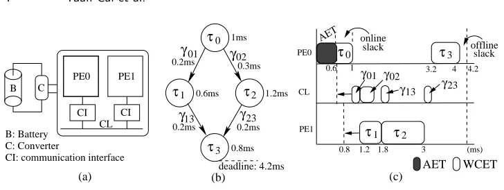
Fig. 1. Task graph and system model

2. PRELIMINARIES

2.1 System Model and Task Graph

We consider battery-powered embedded computing systems, illustrated in Fig. 1(a), which consist of multiple processing elements (PEs) connected by communication links (CLs). A dc/dc converter adapts the battery voltage to the system supply voltage. The system functionality is captured by a task graph model G(T,C), shown in Fig. 1(b). Nodes (τi∈ T) in this directed acyclic graph (DAG) represent computational tasks. Edges (γj ∈ C) denote data communications between tasks. As shown in Fig. 1(b), tasks/edges are associated with worst case execution times (WCETs). The WCETs depend on the worst case number of cycles (Kw) required for execution and the circuit frequency f, which in turn depends on the supply voltageVddand threshold voltageVt [Luo and Jha 2002a]. The following equation gives the relationship between these parameters and the execution time.

t= Kw

f =

Kw·Vdd

k·(Vdd−Vt)α

(1)

where k and αare technology related constants. The power dissipation of a task can be expressed as [Andrei et al. 2004]:

P=f·Ce·Vdd2 (2)

where Ce is the effective switched capacitance of the circuit. Eqs. (1) and (2) provide the well-known energy/delay tradeoff exploited by all DVS procedures. In a battery-powered system, the discharge current drawn from the battery,I, equals

P/(Vb·η), whereVbandηare the average battery voltage and the converter efficiency respectively and both can be regarded as constants [Rakhmatov and Vrudhula 2003]. In this paper, we set Vb and η as 5V and 0.9 respectively. Since DVS can reduce the power, P, it can be used to down scale the battery discharge current and achieve savings in the battery charge consumption [Rakhmatov and Vrudhula 2003], [Chowdhury and Chakrabarti 2002]. We assume that tasks and edges have been initially (offline) mapped and scheduled onto the target architecture, such that resource and time constraints are satisfied under WCETs, as illustrated in Fig. 1(c). At run-time, however, tasks might finish before their WCET, resulting in online slack. For instance, in Fig. 1(c)τ0 has an actual execution time (AET) of

0.6ms, leaving an online slack of 0.4ms.

2.2 Battery Model

Rao et al. give a comprehensive survey on battery modeling in [Rao et al. 2003]. In this work we use an analytical high-level battery model proposed in [Rakhmatov and Vrudhula 2003] whose accuracy has been demonstrated to be within 3% of the physical battery. The battery charge consumption at timetis modeled as:

σ(t) =

N−1

X

k=0

Ik·F(t, stk, stk+ ∆k, β) (3)

whereN is the total number of steps used to approximate the load current profile (LCP),t is the time that the battery has been discharged for, andIk, ∆k andstk denote the current, the duration and the start time ofstepkin the LCP, respectively. Further,β is a constant related to the non-linear property modelled by functionF:

F(x, y, z, β) =z−y+ 2 10 X

m=1

e−β2

m2

(x−z)_−e−β2

m2

(x−y)

β2_m2 (4)

If the capacity of the battery isα, then solving equationα=σ(L) will give the bat-tery lifetimeL. Here the values ofαandβ are set to 40375 and 0.273 respectively according to [Rakhmatov and Vrudhula 2003]. Since smaller charge consumption will lead to longer battery lifetime [Rakhmatov and Vrudhula 2003], our optimiza-tion objective is the minimizaoptimiza-tion of the charge consumpoptimiza-tion.

3. PROBLEM FORMULATION

We assume that the tasksT ={τi} and precedence constraintsC ={γj} of task graphG(T,C) have been initially mapped and scheduled onto a distributed archi-tecture containing voltage scalable processors, which can vary their supply voltage

τ

τ

τ

τ

τ

τ

τ

τ

τ

τ

t

(b) (a)

Fig. 2. Office-auto task graph [Dick] and execution order

4. BATTERY-AWARE ONLINE VOLTAGE SCALING 4.1 Motivational Example

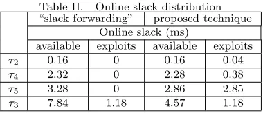
The essence of the online voltage scaling problem is the online slack distribution, in order to efficiently exploit slack resulting from tasks that execute faster than their WCETs. In this motivational example we outline two different slack distribution methods using a realistic task graph from the E3S suite [Dick ], namely the office-auto benchmark consisting of 5 tasks illustrated in Fig. 2(a). For simplicity we consider here that all tasks have been mapped to a single processing element and the execution order corresponds to Fig. 2(b). We assume that the PE can vary its supply voltage betweenVmin andVmax, withVmin= 0.4·Vmax. In accordance, the task execution times follow Eq. (1). Table I gives the worst-case execution time (WCET) and discharge current (I) of each task (in execution order of Fig. 2(b)), when executing at Vmax. Furthermore, the table shows the actual execution time (AET) of tasks at run-time (we assume here 80% of WCET), as well as the resulting online slack (WCET-AET). The deadline is assumed to correspond to the finishing time of the last task (τ3), when all tasks execute with their WCET. Table II shows the outcome of two different techniques that distribute the available online slack. Note that not all the available online slack might be exploited due to the limited voltage range of the PE. The first technique is based on the slack forwarding idea presented in [Ahmed and Chakrabarti 2004], in which all available online slack is forwarded to the last task. Accordingly, task τ3 accumulates an online slack of 7.84ms (0.16+2.16+0.96+4.56) before it starts execution. Nevertheless, due to the limited voltage range of the PE, it is only possible to make use of 1.18ms of the total slack, i.e., 6.66ms of slack remain unexploited. As a result, a battery charge of 0.189mAs is consumed, which is calculated from Eqs. (1)–(4) and the task properties given in Table I. A second approach (the approach we propose in this paper) distributes the available online slack by explicitly considering the discharge currents and WCETs of tasks. That is, each time a task finishes execution, the

Table I. WCETs, discharge currents, AETs and online slacks of auto-office tasks

τ1 τ2 τ4 τ5 τ3

WCET (ms) 0.79 10.80 4.80 22.81 0.79 I(mA) 0.256 4.066 3.990 4.243 0.256

AET (ms) 0.63 8.64 3.84 18.25 0.63

online slack (ms) 0.16 2.16 0.96 4.56 0.16

Table II. Online slack distribution “slack forwarding” proposed technique

Online slack (ms)

available exploits available exploits

τ2 0.16 0 0.16 0.04

τ4 2.32 0 2.28 0.38

τ5 3.28 0 2.86 2.85

τ3 7.84 1.18 4.57 1.18

workload-ahead (sum over products of discharge current and WCET of remaining tasks) is evaluated to make a slack distribution decision. The method is outlined in Section 4.2, however, the resulting slack distribution is given in Table II. As we can observe from the table, using this method all tasks are assigned some of the available slack. For instance, after taskτ1 has finished execution the available online slack that is exploitable by task τ2 is 0.16ms. However, it exploits only 0.04ms of this slack via voltage scaling, while the remaining 0.12ms are accumulated for the workload ahead. Therefore, after τ2 finishes the available slack is 2.28ms (2.16+0.12). As shown in Table II, taskτ4 exploits 0.38ms of this slack. Similarly, the slack is forwarded and distributed to the tasks τ5 and τ3. When τ3 is to be executed, the available online slack (4.57ms) is still sufficient to scale its voltage to the lowest level, i.e. τ3 obtains the same amount of slack then with the slack forwarding approach. According to the second distribution, the consumed battery charge is reduced to 0.154mAs, an improvement of 18.5% when compared to the slack forwarding method [Ahmed and Chakrabarti 2004].

4.2 Workload-Ahead-Driven Online DVS Technique

As we have seen in the motivational example of Section 4.1, slack forwarding is not particularly effective for heterogeneous tasks which draw different currents from the battery and require different WCETs. An effective online DVS algorithm must take these aspects into consideration to achieve a “globally” fair distribution of online slack. To cope with this problem, we define two metrics that capture the effects of tasks on the battery charge consumption. Letτnext be the next task to be executed. DenoteTr the set of tasks that start later thanτnext andτnext itself. Mathematically,Tr={τnext, τi|τi starts later thanτnext}.

Definition 1_{: Theworkload (Wi) of a taskτiis the product of its discharge current} Ii and WCETi, i.e. Wi=Ii·W CETi.

Definition 2_{: Theworkload-ahead (W Ai) of a taskτi is the sum of the workloads}

of all tasks inTr, i.e. W Ai=P_τj∈TrWj.

The workload-ahead-driven slack distribution gives the slack to the next task based on the ratio of itsW andW A:

slacknext=

Wnext

W Anext

·os (5)

the real execution times and can be applied with eitherB orE policies [Rao et al. 2005]. It should be noted that both W and W A for each task are computed in the offline phase, so this computation does not contribute to the online complexity of the algorithm. It is also important to note that it is our aim to develop an effective yet fast online DVS technique, hence we intentionally avoiding a complex online algorithm. Though there exist DVS algorithms that can achieve much lower battery charge consumption ([Rakhmatov and Vrudhula 2003]), the high complexity of these methods prevent them to be utilized in the online phase.

The underlying idea behind of Eq. 5 is based on the battery model, which is described by Eq. 3 and Eq. 4. Substituting Eq. 4 into Eq. 3, we obtain

σ(t) =

N−1

X

k=0

Ik ∆k+ 2 10 X

m=1

e−β2

m2

(t−stk−∆k)_−e−β

2

m2

(t−stk)

β2_m2

!

=

N−1

X

k=0

Ik∆k+ 2

N−1

X

k=0 10 X

m=1

e−β2

m2

(t−stk−∆k)_−e−β

2

m2

(t−stk) β2_m2

Here ∆k is the WCET of taskτk andIk·∆k is the workload of taskτk. Hence a task with larger workload will consume more battery charge and should be scaled more aggressively. This has been reflected in Eq. 5, which gives more slack to a task with larger workload so that the voltage of the task can be more aggressively scaled. Another important factor affecting the battery charge consumption is the position of a task in the schedule (the later a task is in the schedule, the smaller should be the current it draws [Chowdhury and Chakrabarti 2002]). This factor is also taken into account by Eq. 5: the later a task is in the schedule, the smaller its W A, and as a result, it will receive relatively larger slack and its current will be smaller as desired. For example, from Tables I and II we can observe that task

τ5 has the largest workload (22.81ms·2.243mA) and its position is close to the end of the schedule and as a result, it obtains the largest slack portion (2.85ms). Note that we only calculate the slack distributed to the next task. It is not necessary to distribute slack to tasks beyond the next task because the total amount of online slack will change with the execution of the next task, hence, a recomputation of the distribution is required.

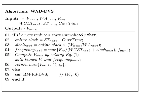
Based on the above outlined workload-ahead principle, Fig. 3 gives the pseudo code of our workload-ahead-driven voltage scaling algorithm. Its input consists of the information regarding the next task. This information includes the task’s workload (Wnext) and workload-ahead (W Anext), its worst case number of cycles (Kw) and execution time (W CETnext), as well as its offline decided start time (STnext). In addition, the algorithm requires the current time (CurrT ime) in the schedule. When a busy PE finishes executing a task or an idle PE receives an incoming data communication, it calls the online voltage scaling algorithm. If the next task on the PE can start immediately (line 1), the available online slack is computed from the current time and the start time of the next taskτnext (line 2). The slack distributed toτnext is calculated based on Eq. (5) in line 3. According to the amount of distributed slack, the frequency and voltage at whichτnext has to be executed are computed in lines 4 and 5. If the resulting frequency is less than the minimum frequency (fmin) of the PE, then the minimum frequency will be used.

Algorithm: WAD-DVS

Input: -Wnext,W Anext,Kw,

W CETnext,STnext,CurrT ime

Output: -Vnext

01: ifthe next task can start immediatelythen 02: online slack=STnext–CurrT ime;

03: slacknext=online slack×(Wnext/W Anext);

04: f requencynext=max{Kw/(W CETnext+slacknext),fmin};

05: Compute Vnextby solving Eq.(1)

with known Vt and f requencynext;

06: return max{Vnext, Vmin};

07: else

08: callRM-RS-DVS; // (Fig. 6) 09: end if

Fig. 3. Pseudo code: Workload-ahead-driven online DVS

If the resulting voltage is larger than the minimum voltage (Vmin) of the PE, it will be returned. Otherwise,Vmin will be returned (line 6). On the other hand, if the next task could not start at this moment due to the lack of needed input data (e.g. τ3 in Fig. 1 (c) can not start whenτ0 finishes sinceγ23 has not arrived yet), the algorithm calls the online task rescheduling/remapping procedure described in Section 5 (line 8). It is important to note that each step in the algorithm can be performed in constant time, hence the overall complexity is constant. The constant complexity allows the scaling overhead be incorporated into the WCET of tasks during timing analysis [Shen et al. 1993]. In the above described online voltage scaling algorithm, no task will start later than its offline decided start time, so the timing constraint of each task is guaranteed and all hard deadlines are satisfied. In the above DVS procedure, we did not consider the time and energy overheads of the voltage transition. The issue of handling the transition overheads has been addressed in [Andrei et al. 2004] and [Mochocki et al. 2005] for offline DVS and online DVS respectively. According to [Mochocki et al. 2005], in the online phase, when a task is ready to be executed, we can subtract the time overhead of the transition from online slack and use the remaining slack as the available slack in our DVS algorithm. If the overhead is equal to or greater than the online slack, the DVS will not be involved. Similarly, we can compare the energy saving of the ready task due to DVS with the energy overhead. If the energy saving is larger, DVS will be called, otherwise, it is rejected. In this paper, however, we omit the transition overheads for simplicity since they are not the focus of this paper.

5. ONLINE TASK RESCHEDULING AND REMAPPING

possible? Re− scheduling

Re−

possible? mapping next task

Information

of the task startCan next now?

Remapping Rescheduling

Perform WAD

PE remains

idle

No No

No

Yes Yes Yes

Fig. 4. Integrated workload-ahead-driven DVS and rescheduling/remapping

τ₁

τ3

τ1

τ6

τ3

τ4

AET WCET

τ6

τ4 τ2 τ0

1ms

τ5

1ms

τ5

os

(a) (b)

PE2 PE1 PE0

remapping rescheduling

1 3.5 4.5 7 8 10 (ms)

wasted without rescheduling or remapping

2ms

1ms usable_slack

not

4.5ms _4ms

2ms

τ2

τ0

Fig. 5. Online task rescheduling and remapping

remapping as supplements of the proposed online DVS (Section 4.2). Fig. 4 outlines the integration of the workload-ahead-driven DVS technique with the rescheduling and remapping strategy. The necessity for online rescheduling and remapping is illustrated through a motivational example.

5.1 Motivational Example

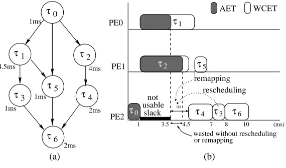
Fig. 5(a) shows a task graph consisting of 7 nodes. The WCETs of tasks are indicated, and the tasks are mapped and scheduled on 3 PEs, in accordance to Fig. 5(b). For simplicity we neglect communications in this example, however, they are considered in our algorithm. As we can observe from Fig. 5(b),τ1has a longer WCET (4.5ms) thanτ2 (4ms). However, let us assume thatτ1 requires only 2.5ms for execution at run-time, i.e. it finishes at 3.5ms. When τ1 finishes, there is an online slack appearing on PE2 (indicated as os in Fig. 5(b)), butτ4 can not start its execution earlier because its parent taskτ2has not terminated at this moment. Clearly, a large portion of the online slack on PE2 is wasted. To avoid this waste, task τ3 on PE2 can be placed before τ4 to fill the available online slack. That is, we change the execution order of the remaining tasks (rescheduling). However, the WCET of the rescheduled task must be smaller than the available online slack to avoid the delay of the start time of the remaining tasks, which could result in

Algorithm: RM-RS-DVS

Input: -Wnext,W Anext,W CETnext,STnext,Kw,

CurrT ime,M Output: -Vnext

01: intk = min(M, size of P E[p].exe Queue); 02: boolsearch result = f alse;

03: forj = 1tok //online rescheduling

04: ifP E[p].exe Queue[j]satisf ies rescheduling conditionsthen 05: search result = true;

06: move P E[p].exe Queue[j]to the head of P E[p].exe Queue; 07: break;

08: end if 09: end for

10: ifsearch result == truethen 11: callWAD-DVS; // (Fig. 3) 12: else// online remapping 13: fori = 1ton&&i! = p

14: k = min(M, size of P E[i].exe Queue); 15: forj = 1tok

16: ifP E[i].exe Queue[j]satisf ies remapping conditionsthen 17: search result = true;

18: f etch task P E[i].exe Queue[j]f rom P E[i]and put it to the head of P E[p].exe Queue;

19: break;

20: end if 21: end for

22: ifsearch result == truethen 23: break;

24: end if 25: end for

26: ifsearch result == truethen 27: callWAD-DVS; // (Fig. 3) 28: else

29: let P E[p]be idle; 30: end if

31: end if

Fig. 6. Pseudo code: Online rescheduling/remapping

potential deadline violations. For example, to be rescheduled, the WCET of τ3 must be smaller thanos. If the WCET ofτ3 is longer than the slack, then we can further search the remaining tasks of other PEs to see if there is suitable task. In the example of Fig. 5(b),τ5on PE1 can be fetched from PE1 to fill the online slack on PE2, i.e.,τ5 is remapped online.

5.2 Online Task Rescheduling and Remapping Technique

pseudo code of our online task rescheduling/remapping is given in Fig. 6. Suppose there are n PEs in the system and the pth (1 ≤p ≤ n) PE is the one with the potentially wasted online slack. Let each PE have anexe Queuestoring tasks to be executed and letM be a constant integer called the search window size. The search window size represents the maximal number of tasks in exe Queue that may be rescheduled or remapped. The complexity of the algorithm is bounded by the search window size, which is constant. The algorithm first restricts the search window size if the number of tasks in exe Queueis smaller thanM (line 1), then searchesexe Queueof PE[p] within the search windowM to fill the online slack on PE[p]. To be a rescheduling candiate, a task should satisfy two conditions (line 4). First, its WCET (we still only know WCET of remaining tasks at this moment) is less than the online slack so that the next task will start no later than its offline decided start time. For example, in Fig. 5, the WCET ofτ3 is less than the online slack andτ4 is guaranteed to start on time. This condition prevents any deadline violation. The second condition is that at the time of the search, all its incoming data communications have arrived so that it can start at this moment. If these two conditions are true, the found task is moved to the head of the execution queue and placed before the next taskτnext (line 6). Then the proposed online DVS pro-cedure is called (line 11) to utilize the otherwise wasted online slack. As indicated in Fig. 4, if no suitable task for rescheduling has been found, task remapping will be performed (line 12-31). Similar to online rescheduling, online remapping checks tasks in the search window ofexe Queueof other PEs to find a task that can utilize the available online slack (line 12-22). Nevertheless, the selection is more strict in remapping phase (line 16). Tasks can only be fetched from another PE if they fulfill the two conditions mentioned in the rescheduling phase as well as if their remapping does not introduce new communications. The reason is that new data communications may delay the transfer of some other scheduled communications on the CLs. This, in turn, may cause some tasks not to start on time and result in the risk of deadlines violation. After a task is remapped it is removed from the task queue of its originally mapped PE toexe Queuehead of PE[p] (line 18), which then will call the proposed voltage scaling procedure (line 27). If no task can be found remappable, the idling of PE[p] is not avoided and the online slack is wasted (line 29).

The complexities of the rescheduling and remapping algorithms are O(M) and

O(n×M) respectively, whereM is the search window size andnis the number of PEs. NeitherM norn will change at runtime, resulting in a constant complexity of the rescheduling/remapping algorithm. Usually,n is a small integer and as we will see in Section 7, the search window size is also a small number, hence the computational overhead of the rescheduling/remapping algorithm is very low.

6. COMBINED ONLINE DVS AND ABB

In Section 4, we mainly considered the dynamic power, which has been the dominant source of power consumption in contemporary CMOS digital systems. However, with ever-shrinking feature sizes, leakage power is becoming comparable to dynamic power [Martin et al. 2002]. For the 0.05µm predictive technology, the leakage power is estimated to be almost equivalent to the dynamic power [Yan et al. 2003].

Though DVS can decrease the dynamic power significantly, it is not very effective in reducing leakage power. To tackle this problem, adaptive body biasing (ABB) has been introduced. ABB takes advantage of the fact that the leakage current can be exponentially reduced by dynamically changing the body-bias voltage (Vbb) of transistors [Keshavarzi et al. 2001]. A microprocessor prototype which can change

Vbb continuously was introduced in [Miyazaki et al. 2002]. Kim and Roy proposed a scheme to scaleVbb, which can be included in any processor [Kim and Roy 2002]. In order to minimize the overall power, combined DVS and ABB can be utilized [Martin et al. 2002], [Yan et al. 2003], [Andrei et al. 2005]. In this section, we extend the workload ahead-driven DVS technique introduced in Section 4 towards the consideration of the leakage power, i.e., we combine DVS and ABB (referred to DVSABB from now on) to achieve power efficiency in terms of leakage and dynamic power.

The leakage power is mainly caused by subthreshold leakage currents in the CMOS circuitry and it can be modeled as [Martin et al. 2002]

Pleakage=Vdd·K3·eK4Vdd·eK5Vbs (6)

where Vbs is the body-bias voltage and the fitting parameters K3, K4, K5 are technology dependent constants. For clarity reasons we maintain the same indices as used in [Martin et al. 2002]. Actual values for these constants are provided in [Martin et al. 2002], given a Transmeta Cruose processor. Considering Eq.2, the total power of one task can then be expressed as

Ptotal=Pdynamic+Pleakage=f ·Ce·Vdd2 +Vdd·K3·eK4Vdd·eK5Vbs (7)

The operational frequencyf depends onVddas well asVbsand can be expressed as [Martin et al. 2002]

f = ((1 +K1)·Vdd+K2·Vbs−Vth1) α

K6·Ld·Vdd

(8)

whereLd is the logic depth, andα,K1,K2,K6 andVth1denote circuit dependent constants [Martin et al. 2002]. From Eq.7, we can find that scalingVdd(DVS) and

depends nonlinearly onVddandVbs(Eq. 7), this results in a nonlinear optimization problem. Numerical methods that are commonly used to address such optimiza-tion problems are unsuitable for online techniques due to their large time overhead compared to the application running on the system. Therefore, we utilize the idea of a look-up-table (LUT) approach proposed by [Andrei et al. 2005] to solve the problem.

In this approach, each task will have a specific LUT which is set up before the actual execution (i.e., in the offline phase). Each entry of the LUT corresponds to a possible slack that the task may have. A pair of Vdd and Vbs are pre-computed based on this slack and stored in this entry. Then in the online phase, each time when a task is to be executed, the PE will look up the voltage pair in the LUT according to the actual online slack obtained by the task. In the LUT, the step between two entries is a constant. For a given slack, we can use ⌈slack

step⌉ to find its entry. For example, the slacks in the table are 0, 0.2, 0.4, 0.6, 0.8 ms and the step is 0.2ms. If the slack distributed to the next task is 0.5ms, then ⌈0.5_0.2⌉ = 3, i.e., (Vdd, Vbb) in the 3rd entry will be used. Since this entry found procedure is quite simple, the overhead due to the table lookup is very small and constant. If the actual slack falls between two entries of the LUT, the voltage pair in the lower entry will be simply used. Though this is conservative and the slack is not fully used, the time-constraint will be guaranteed. The space complexity of the LUTs depends on the number of tasks,T, and the average number of entries of one table,

E. We assume it takes 4 bytes to store the slack,VddandVbsrespectively, then the space to store the LUTs will be 12×E×T. For example, ifE= 20 andT = 100, then the LUTs needs 24,000 bytes (approximately 23.44 KB) memory.

The LUT setup procedure is outlined next. First, we compute the possible online slack range of each task, i.e., the difference between the worst case slack (WCS) and the best case slack (BCS) that each task may have. The WCS that every task would have is clearly zero. This is the case where all tasks are executed with their WCETs. We assume each task will obtain the BCS when the AETs of all tasks are 30 percent of their WCETs. For each task, the LUT is set to be empty initially, then starting from its WCS, we add entries to its LUT with certain interval until its BCS is reached. Hence each entry of the LUT corresponds to a possible slack that the task may obtain at run time. For each entry, we use exhaustive search to find the optimal pair of (Vdd,Vbs) . Letpbe the percentage of the slack distributed to DVS, then 1−p percent of slack will be given to ABB. We change p from 0 to 100 percent with an interval of 1 percent. With eachp, a pair of (Vdd, Vbs) is computed according to Eq.8. Then we calculate the total powerPtotalbased on the computed voltage pair and Eq.7. The voltage pair corresponding to the minimum

Ptotalis the optimal pair and will be chosen to fill the table entry. The computation

of (Vdd,Vbs) is repeated until every entry of the LUT is filled. It can be seen that the above LUT setup procedure is time consuming, but the setup speed is not our concern since the it is carried out in the offline phase. Once the tables are set up, the online lookup will be very fast and the complexity isO(1).

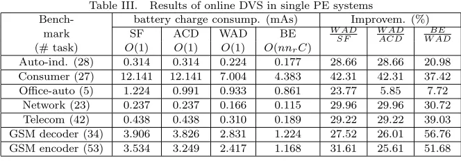
Table III. Results of online DVS in single PE systems

Bench- battery charge consump. (mAs) Improvem. (%)

mark SF ACD WAD BE W AD_SF W AD_{ACD W AD}BE

(# task) O(1) O(1) O(1) O(nnrC)

Auto-ind. (28) 0.314 0.314 0.224 0.177 28.66 28.66 20.98 Consumer (27) 12.141 12.141 7.004 4.383 42.31 42.31 37.42 Office-auto (5) 1.224 0.991 0.933 0.861 23.77 5.85 7.72

Network (23) 0.237 0.237 0.166 0.115 29.96 29.96 30.72 Telecom (42) 0.438 0.438 0.310 0.189 29.22 29.22 39.03 GSM decoder (34) 3.906 3.826 2.831 1.224 27.52 26.01 56.76 GSM encoder (53) 3.534 3.249 2.417 1.168 31.61 25.61 51.68

7. EXPERIMENTAL RESULTS

In order to validate the effectiveness of the proposed online voltage scaling and rescheduling/remapping strategies in reducing battery charge consumption, we con-ducted several experiments using 15 hypothetical examples as well as 7 real-world benchmakrs. The hypothetical examples have been automatically generated using TGFF [Rhodes and Dick ], a pseudo-random task graph generator. The first 5 real-istic examples have been taken from the E3S benchmark suit [Dick ] (auto-indust, consumer, office-auto, networking and telecomm), while the task graphs for GSM decoder and encoder have been derived from publicly available C code [Schmitz ]. All reported results have been obtained using the battery model of Section 2.2 and the evaluation criterion is the battery charge consumption. Further, the evaluation is based on the same normal distribution (mean: 0.6 times the WCET, standard deviation: 0.13 times the WCET) of the actucal execution times of tasks that has been used in [Ahmed and Chakrabarti 2004].

In the first set of experiments, we evaluate the efficiency of our workload-ahead-driven DVS algorithm (WAD, Fig. 3) by means of a comparison with 4 different online DVS techniques, summarized for reference in the following: 1. SF_{: The}

slack forwarding approach is based on the technique presented in [Ahmed and Chakrabarti 2004]. Its time complexity is constant (O(1)). 2. ACD_{: The average}

current-based distribution is a heuristic that leverages information regarding the task discharge currents to distribute slack: if the current of the next task to be executed is less than or equal to average current of tasks, it gets no slack; else, it gets some slack such that its current decreases to the average value. When there is only one task left, all slack is assigned to it. The time complexity of this method is constant, too. We use this heuristic to underline the importance of the workload-driven technique that considers discharge currents as well as remaining task execution times. 3. WAD_{: This represents our workload-ahead-driven}

distri-bution technique, as introduced in Section 4.2. It has also a complexity of O(1). Since the slack forwarding idea [Ahmed and Chakrabarti 2004] is most suitable for task sets without data communications, we executed the 7 realistic benchmarks on single PE systems1_{, in which the inter-PE communications between tasks can be} neglected. 4. BE_{: A best effort slack distribution adapted from an offline DVS}

1_{Note that not all these benchmarks can be executed on a single PE without violating timing}

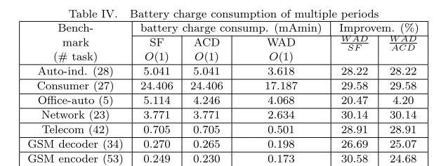
Table IV. Battery charge consumption of multiple periods Bench- battery charge consump. (mAmin) Improvem. (%)

mark SF ACD WAD W AD_SF W AD_ACD

(# task) O(1) O(1) O(1)

Auto-ind. (28) 5.041 5.041 3.618 28.22 28.22

Consumer (27) 24.406 24.406 17.187 29.58 29.58

Office-auto (5) 5.114 4.246 4.068 20.47 4.20

Network (23) 3.771 3.771 2.634 30.14 30.14

Telecom (42) 0.705 0.705 0.501 28.91 28.91

GSM decoder (34) 0.270 0.265 0.198 26.69 25.07

GSM encoder (53) 0.249 0.230 0.173 30.58 24.68

procedure of [Rakhmatov and Vrudhula 2003]. It divides the online slack into small steps. For each step, every remaining task is tried to be scaled by using this step of slack and the task which can cause the minimum battery charge consumption will be assigned with this step. This procedure is repeated until all the steps are dis-tributed, i.e., the available online slack is used up. The complexity of this method isO(nnrC), wherenis the number of all tasks,nr is the number of the remaining tasks and C is the number of slack steps. This technique can achieve much lower battery charge consumption than the above three heuristics due to the complicated search it uses. However, its high complexity prevents it to be utilized at run-time

Table III gives the results of the four different DVS methods in terms of bat-tery charge consumption. In the table, the first column gives the benchmark name and the number of tasks in the benchmark. The results of the four online DVS techniques are given in Columns 2–5. In columns 6-7, we show the percentage of improvement in battery charge consumption using the proposed WAD method over methods SF and ACD. The improvement of BE over WAD is given in the last column. Consider, for instance, the GSM decoder benchmark. Here BE ob-tains the minimum battery charge consumption of 1.224mAs. SF and ACD result in 3.906 mAs and 3.826mAs, respectively and WAD achieves 2.831mAs, resulting in improvements of 27.52% and 26.01% over SF and ACD. We can observe that BE yields consistently the lowest battery charge consumption among the four tech-niques, but its computational complexity is also much higher than the other three. Among the three heuristics with constant complexity, WAD achieves lower battery charge consumption than SF and ACD. Table III gives the battery charge consump-tion that the applicaconsump-tions run for one period. We also repeat the experiments of the three heuristics with constant complexity for several thousand periods so that the total operation time reaches the scale of minutes. The resulting battery charge consumptions are shown in Table IV. From this table we can find that WAD is still more effective than SF and ACD.

The second set of experiments was conducted to validate the workload-ahead-driven DVS as well as the rescheduling/remapping techniques in the context of systems consisting of multiple processing elements. We used LOPOCOS [Schmitz et al. 2002], an academic system-level synthesis tool, to find suitable multiple PE im-plementations and to generate the offline mappings and schedules for all 36 bench-marks (GSM decoder and encoder have been combined into a single benchmark). In all experiments we set the search window size (M) of the rescheduling/remapping

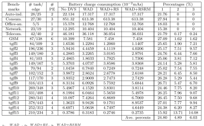
Table V. Experimental results in multi-PE systems

Bench- # task/ # Battery charge consumption (10−2_{mAs) Percentages (%)}

marks edge PE No DVS WAD WAD+RS WAD+RSRM 1 2 3

Auto-ind. 28/25 2 22.134 17.317 17.317 17.317 21.76 0 0

Consum. 27/30 3 851.32 613.38 613.38 613.38 27.94 0 0

Office-au. 5/5 1 15.578 12.768 12.768 12.768 18.03 0 0

Network. 23/19 2 12.295 10.404 10.404 10.404 15.38 0 0

Telecom. 42/40 2 46.181 36.118 36.054 36.031 21.79 0.17 0.24

GSM 87/138 6 10.399 7.581 7.458 7.458 27.09 1.62 1.62

tgff1 84/109 3 1.6536 1.2294 1.2060 1.1407 25.65 1.90 7.21

tgff2 196/236 3 5.9416 4.4459 4.1119 4.0206 25.17 7.51 9.57

tgff3 149/180 3 4.2885 3.2265 3.0185 2.9791 24.76 6.44 7.66

tgff4 81/103 3 2.4865 1.8633 1.7925 1.7306 25.06 3.81 7.12

tgff5 149/167 5 5.3703 4.0737 3.8586 3.8368 24.14 5.28 5.81

tgff6 70/94 2 1.0458 0.7840 0.7249 0.7248 25.02 7.54 7.55

tgff7 102/152 3 3.9872 2.8624 2.6778 2.6188 28.21 6.45 8.50

tgff8 117/170 3 3.9352 2.9009 2.7473 2.7429 26.28 5.29 5.44

tgff9 316/413 4 8.3134 6.0926 5.7592 5.6844 26.71 5.47 6.70

tgff10 269/348 3 5.4967 4.1520 3.8301 3.8114 24.46 7.75 8.20

tgff11 331/408 4 8.1994 6.0464 5.5650 5.4978 26.25 7.96 9.07

tgff12 280/341 4 10.097 7.4264 6.8689 6.7069 26.45 7.50 9.68

tgff13 378/443 4 1.3623 9.9426 9.1701 8.9537 27.01 7.77 9.94

tgff14 252/312 4 6.6971 5.0638 4.7497 4.6449 24.38 6.20 8.27

tgff15 210/234 3 0.3786 0.3183 0.2746 0.2735 15.92 13.71 14.08

Ave. percents 24.80 4.89 6.03

1: _{N oDV S}W AD ; 2: W AD_{W AD}+RS; 3: W AD_{W AD}+RSRM

algorithm to 10, empirically found to be a good value. Nevertheless, due to the importance of the window size on the solution quality we have devoted an extra set of experiments on this subject, presented later in this section. Since the slack forwarding technique [Ahmed and Chakrabarti 2004] was particularly introduced for independent tasks, we refrain in these experiments from a direct comparison.

The results of our experiments are summarized in Table V. The first, second, and third columns give the benchmark name, the number of tasks/communication edges, and the number of PEs in the system, respectively. Columns 4–7 show the battery charge consumptions in 4 different scenarios. Column 4 (No DVS) repre-sents the nominal charge consumption, i.e., when no online voltage scaling is em-ployed; Column 5 (WAD) shows the results of the proposed workload-ahead-driven DVS technique; Columns 6 (WAD+RS) and 7 (WAD+RSRM) give the charge con-sumption when integrating WAD with online rescheduling and rescheduling with remapping, respectively. Columns 8–10 summarize the achieved battery charge sav-ings in percent. Consider, for instance, benchmark tgff2. Here the nominal and the WAD-based charge consumptions are 5.941610×10−2_{mAs and 4.4459×10}−2_mAs, respectively, representing a saving of 25.17%. This can be further improved by using rescheduling as well as rescheduling with remapping to 4.1119×10−2_{mAs and} 4.0206×10−2_{mAs, respectively, obtaining further saving of 7.51% and 9.57% when} compared to using WAD only.

−2

6.6 6.8 7 7.2 7.4 7.6 7.8

0 1 2 3 4 5 6 7 search window size (M)

battery charge conumption

battery charge consumption (10 mAs)

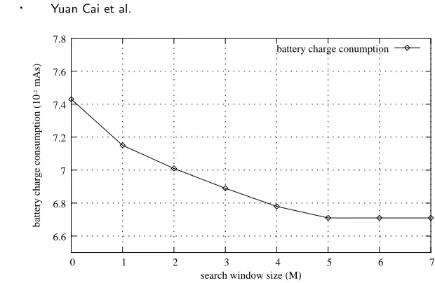
Fig. 7. Influence of search window size on rescheduling/remapping results

technique has an influence on the achievable savings in battery charge consumption as well as on the online complexity. The following experiment is used to clarify this aspect and to provide an insight into which window size should be typically used. Fig. 7 shows the battery charge consumption of benchmark tgff12 depending on the window size M. As it can be observed, a window size of zero, i.e. no reschedul-ing/remapping is performed, results in a charge consumption of 7.43×10−2_mAs. However, with an increasing window size this value decreases to 6.7×10−2_{mAs. In} general, we have observed that for all investigated benchmarks, the window size is no larger than 10.

The above experiments were also repeated for 10 thousand times and the overall schedule lengths reach the scale of minutes and the results are given in Table VI. From this table, it can be seen that the online DVS still achieves remarkable battery charge saving compared to the situation where there is no DVS. While averagely, the rescheduling/remapping algorithms do not further reduce the battery charge consumption too much, they are effective in some benchmarks, for instance, more than 10 percent battery charge can be saved in tgff15 by using rescheduling or remapping. Hence,the rescheduling/remapping algorithm can still be utilized in certain applications.

The third set of experiments was carried out to evaluate the effectiveness of the proposed online DVSABB when the leakage power is taken into account. In the sinlge PE systems, we compare the online DVSABB with the online DVS. The proposed LUT based DVSABB (DVSABB LUT) is also compared with the opti-mal DVSABB obtained through exhaustive search (DVSABB ES). All three scaling methods are workload-ahead-driven. Initially, we assume that before scaling the leakage power of each task is equal to its dynamic power, a realistic assumption for the next generation technology [Yan et al. 2003], and the results are shown in Table VII. We generalize this assumption in a later experiment. The battery charge consumption of the three scaling approaches are given in columns 2-4 and column 5

Table VI. Experimental results in multi-PE systems with multiple periods

Bench- # task/ # Battery charge consumption (mAmin) Percentages (%)

marks edge PE No DVS WAD WAD+RS WAD+RSRM 1 2 3

Auto-ind. 28/25 2 88.858 59.580 59.580 59.580 32.95 0 0

Consum. 27/30 3 916.53 777.34 777.34 777.34 15.19 0 0

Office-au. 5/5 1 18.780 15.289 15.289 15.289 18.59 0 0

Network. 23/19 2 29.450 20.653 20.653 20.653 29.87 0 0

Telecom. 42/40 2 57.569 43.400 43.327 43.311 24.61 0.17 0.21

GSM 87/138 6 11.576 7.725 7.601 7.601 33.26 1.61 1.61

tgff1 84/109 3 4.918 2.982 2.931 2.702 39.37 1.71 9.39

tgff2 196/236 3 10.156 6.399 5.911 5.658 36.99 7.63 11.58

tgff3 149/180 3 8.501 5.265 4.938 4.810 38.07 6.21 8.64

tgff4 81/103 3 6.515 4.032 3.891 3.668 38.11 3.50 9.03

tgff5 149/167 5 10.047 6.240 5.906 5.804 37.89 5.35 6.98

tgff6 70/94 2 3.918 2.457 2.303 2.301 37.29 6.26 6.35

tgff7 102/152 3 7.419 4.412 4.134 4.021 40.53 6.30 8.86

tgff8 117/170 3 7.893 4.735 4.498 4.442 40.01 5.02 6.19

tgff9 316/413 4 12.159 7.501 7.093 6.913 38.31 5.44 7.83

tgff10 269/348 3 9.832 6.137 5.680 5.631 37.58 7.45 8.24

tgff11 331/408 4 11.861 7.507 6.915 6.756 36.71 7.88 10.00

tgff12 280/341 4 13.644 8.631 7.981 7.588 36.74 7.53 12.08

tgff13 378/443 4 16.431 10.664 9.832 9.495 35.10 7.79 10.96

tgff14 252/312 4 10.982 6.935 6.510 6.285 36.85 6.12 9.37

tgff15 210/234 3 1.686 1.340 1.156 1.140 20.52 13.73 14.89

Ave. percents 33.34 4.96 6.61

1: _{N oDV S}W AD ; 2: W AD_{W AD}+RS; 3: W AD_{W AD}+RSRM

shows the improvement of DVSABB LUT over DVS. It can be seen that when the leakage power is considered, DVSABB LUT is more effective than DVS in reduc-ing the battery charge consumption. For example, in the Auto-indust benchmark, DVS achieves the battery charge consumption of 0.973 mAs while DVSABB LUT consumes only 0.715 mAs, resulting an improvement of 26.53%. Although DVS-ABB ES can obtain even lower battery charge consumption, its high run time overhead prevents it to be used online. More importantly, from Table VII it can be seen that the results of DVSABB LUT are quite close to that of DVSABB ES. This demonstrates the high quality of DVSABB LUT which is fast enough to be involved online.

Table VII. Results of online DVSABB in single PE systems

Benchmark battery charge consump. (mAs) Improvemment (%) (# task) DVSonly DVSABB LUT DVSABB ES DV SABB LU T_{DV Sonly}

Auto-ind. (28) 0.973 0.715 0.697 26.53

Consumer (27) 9.337 6.684 6.464 28.41

Office-auto (5) 0.574 0.494 0.490 13.86

Network (23) 0.395 0.317 0.313 19.87

Telecom (42) 0.875 0.627 0.613 28.38

GSM decoder (34) 22.22 16.86 16.58 24.11

GSM encoder (53) 31.70 22.92 22.37 27.39

Table VIII. Effectiveness of DVSABB with different leakage/dynamic ratio Pleakage/Pdynamic

Benchmark (more leakage power<————->more dynamic power)

(# task) 1.5 1.25 1 0.75 0.5 0.25

Auto-ind. (28) 33.37 29.65 26.53 18.91 12.50 2.51 Consumer (27) 34.05 31.25 28.41 23.44 12.83 3.58 Office-auto (5) 18.73 15.17 13.86 7.53 6.27 1.58 Network (23) 32.68 26.23 19.87 13.34 9.47 2.55 Telecom (42) 32.75 30.31 28.38 21.83 13.05 2.91 GSM decoder (34) 38.32 33.71 24.11 20.84 11.72 1.97 GSM encoder (53) 34.12 29.40 27.39 22.49 13.83 3.01

25% of the dynamic power, ABB technique is not necessary and we can utilize DVS solely. On the other hand, when the ratio is above 1, which represents the case of the incoming technologies (0.05µmand below), much more battery charge can be saved by combining DVS with ABB, e.g., in the Auto-ind. benchmark, DVSABB can save 33.37% battery charge compared to only DVS when the leakage power is 1.5 times of the dynamic power.

We also compare the workload-ahead-driven DVSABB (WAD DVSABB) with DVSABB combined with slack forwarding (SF DVSABB) and the results are sum-marized in Table IX. After the online DVS is extended to online DVSABB, the proposed WAD approach also performs better than SF in terms of battery charge consumption, with up to 50% improvement.

Finally, we implement the DVSABB technique in the multiple PE systems and in-tegrate it with online rescheduling and remapping. We compare the DVSABB with DVS in two frames: with rescheduling (RS); with both rescheduling and remap-ping (RSRM), and assume that for each PE, the leakage power equals the dynamic power. The battery charge consumptions and the improvement of DVSABB over DVS are summarized in Table X. From the table we can see that in each frame, DVSABB results in lower battery charge consumption compared to DVS in both RS case and RSRM case. This indicates that DVSABB is also more effective than DVS in reducing the battery charge consumption in the multiple PE systems, with up to 29% improvement.

Table IX. Comparison of WAD DVSABB with SF DVSABB Benchmark battery charge consump. (mAs) Improvemment (%)

(# task) WAD SF W AD_SF

Auto-ind. (28) 0.715 1.407 49.17

Consumer (27) 6.684 13.59 50.82

Office-auto (5) 0.494 0.718 31.16

Network (23) 0.317 0.494 35.93

Telecom (42) 0.626 1.186 47.16

GSM decoder (34) 16.863 31.178 45.91

GSM encoder (53) 22.928 41.356 44.56

Table X. Results of online DVSABB in multiple PE systems

Bench- RS RS+RM

marks DVS DVSABB Imp.(%) DVS DVSABB Imp.(%)

Auto-ind. 28.516 25.917 9.11 28.516 25.917 9.11

Consumer 925.78 787.78 14.91 925.78 787.78 14.91

Office-au. 57.395 49.441 13.86 57.395 49.441 13.86

Network. 15.419 12.330 20.03 15.419 12.330 20.03

Telecom. 51.904 42.179 18.74 51.853 42.092 18.81

GSM 17.010 11.977 29.59 17.010 11.977 29.59

tgff1 1.6245 1.3233 18.55 1.4975 1.2298 16.48

tgff2 5.4656 4.5889 16.04 5.1114 4.3027 14.70

tgff3 4.0303 3.4909 13.38 4.0248 3.3696 16.26

tgff4 2.6146 2.1238 18.77 2.6146 2.0979 19.76

tgff5 5.4529 4.4664 18.09 5.3567 4.3950 17.64

tgff6 1.0527 0.8846 15.97 1.0527 0.8846 15.97

tgff7 3.8230 3.2150 15.90 3.6591 3.0970 14.70

tgff8 3.9305 3.3675 14.33 3.9270 3.3541 14.57

tgff9 7.7105 6.7814 12.05 7.1859 6.4756 9.21

tgff10 5.2881 4.6182 12.67 5.1270 4.4986 11.88

tgff11 7.5737 6.4379 15.00 7.3026 6.2677 13.66

tgff12 9.3853 7.8316 16.55 8.9440 7.4716 15.69

tgff13 1.2847 1.0868 15.40 1.2226 1.0516 13.31

tgff14 6.5825 5.5682 15.41 5.5939 5.2927 9.82

tgff15 0.3499 0.3142 10.20 0.3481 0.3128 10.15

8. CONCLUSION

be obtained when compared to approaches that delay the slack utilization as late as possible. All proposed online techniques are extended to combine the adaptive body biasing with dynamic voltage scaling so that the leakage power can also be effectively reduced.

ACKNOWLEDGMENTS

This work is supported in part by the EPSRC, U.K., under grant GR/S95770, the authors would like to acknowledge this support. The authors also wish to acknowledge the reviewers for their comments based on which we could improve the clarity of this work.

REFERENCES

Ahmed, J. and Chakrabarti, C.2004. A dynamic task scheduling algorithm for battery powered

dvs systems. InProceedings of Int. Symp. Circuits and Systems. 813–816.

Andrei, A., Schmitz, M. T., Eles, P., Peng, Z.,and Al-Hashimi, B. M.2004.

Overhead-conscious voltage selection for dynamic and leakage energy reduction of time-constrained sys-tems. InProceedings of Design, Automation and Test in Europe Conf.518–523.

Andrei, A.,Schmitz, M. T.,Eles, P.,Peng, Z.,and Al-Hashimi, B. M. 2005. Quasi-static

voltage scaling for energy minimization with time constraints. InProceedings of Design, Au-tomation and Test in Europe Conf.514–519.

Aydin, H.,Melhem, R.,Mosse, D.,and Mejia-Alvarez, P.2001. Dynamic and aggressive

scheduling techniques for power-aware real-time systems. InProceedings of Real-Time System Symp.95–105.

Chowdhury, P. and Chakrabarti, C.2002. Battery aware task scheduling for a

system-on-a-chip using voltage/clock scaling. In Proceedings of IEEE Workshop on Signal Processing Systems. 201–206.

Dick, R. E3s benchmark suite. http://www.ece.northwestern.edu/ dickrp/e3s/.

Keshavarzi, A.,S. Ma, S. N.,Blocechel, B.,K. Mistry, T. G.,Borkari, S.,and De, V.2001.

Effectiveness of reverse body bias for leakage control in scaled dual-vt cmos ics. InProceedings of Int. Symp. Low Power Electronics and Design. 207–212.

Kim, C. H. and Roy, K.2002. Dynamic vT Hscaling scheme for active leakage power reduction.

InProceedings of Design, Automation and Test in Europe Conf.163–167.

Kim, W.,Shin, D.,Yun, H. S.,Kim, J.,and Min, S. L.2002. Performance comparison of dynamic

voltage scaling algorithms for hard real-time systems. InProceedings of IEEE Real-Time and Embedded Technology and Applications Symp.219–228.

Luo, J. and Jha, N. K.2001. Battery-aware static scheduling for distributed real-time embedded

systems. InProceedings of IEEE Design Automation Conf.444–449.

Luo, J. and Jha, N. K. 2002a. Low power distributed embedded systems: Dynamic voltage

scaling and synthesis. InProceedings of the International Conference on High Performance Computing.

Luo, J. and Jha, N. K.2002b. Static and dynamic variable voltage scheduling algorithms for

real-time heterogeneous distributed embedded systems. InProceedings of Asia and South Pacific Design Automation Conf.712–719.

Martin, S.,Flautner, K., Mudge, T.,and Blaauw, D. 2002. Combined dynamic voltage

scaling and adaptive body biasing for lower power microprocessors under dynamic workloads. InProceedings of IEEE/ACM Int. Conf. Computer-Aided Design. 721–725.

Miyazaki, M.,Ono, G.,and Nagamatsu, T.2002. A 1.2-gips/w microprocessor using

speed-adaptive threshold-voltage cmos with forward bias.IEEE Trans. on Solid-State Circuits 37,2, 210–217.

Mochocki, B.,Hu, X. S.,and Quan, G.2005. Practical on-line dvs scheduling for fixed-priority

real-time systems. InProceedings of IEEE Real-Time and Embedded Technology and Applica-tions Symp.224–233.

Pillai, P. and Shin, K. G.2001. Real-time dynamic voltage scaling for low-power embedded operating systems. InProceedings of ACM Symp. Operating Systems Principles. 89–102.

Rakhmatov, D. and Vrudhula, S.2003. Energy management for battery-powered embedded

systems. ACM Trans. on Embedded Computing Systems 2,3, 277–324.

Rao, R.,Vrudhula, S.,and Chang, N. 2005. Battery optimization vs energy optimization:

Which to choose and when? InProceedings of IEEE/ACM Int. Conf. Computer-Aided Design. 438–444.

Rao, R.,Vrudhula, S.,and Rakhmatov, D.2003. Battery modeling for energy-aware system

design. IEEE Computer 36,12, 77–87.

Rhodes, D. and Dick, R. Task graph for free (tgff). http://ziyang.ece.northwestern.edu/tgff/.

Schmitz, C. Gsm phone task graphs. http://kbs.cs.tu-berlin.de/ jutta/toast.html.

Schmitz, M. T. and Al-Hashimi, B. M.2001. Considering power variations of dvs processing

elements for energy minimization in distributed systems. InProceedings of Int. Symp. System Synthesis. 250–255.

Schmitz, M. T.,Al-Hashimi, B. M.,and Eles, P.2002. Synthesizing energy-efficient embedded

systems with lopocos. Design Automation for Embedded Systems 6, 401–424.

Shen, C.,Ramamritham, K.,and Stankovic, J. A.1993. Resource reclaiming in multiprocessor

real-time systems. IEEE Trans. on Parallel and Distributed Systems 4,4, 382–397.

Shin, D. and Kim, J.2001. A profile-based energy-efficient itra-task voltage scheduling algorithm

for hard real-time applications. InProceedings of Int. Symp. Low Power Electronics and Design. 271–274.

Wu, D.,Al-Hashimi, B. M.,Schmitz, M. T.,and Eles, P.2005. Power-composition profile

driven co-synthesis with power management selection for dynamic and leakage energy reduction. InProceedings of Euromicro Digital System Design. 34–41.

Yan, L.,Luo, J.,and Jha, N. K.2003. Combined dynamic voltage scaling and adaptive body

bi-asing for heterogeneous distributed real-time embedded systems. InProceedings of IEEE/ACM Int. Conf. Computer-Aided Design. 30–37.

Ye, W. and Ernst, R.1997. Embedded program timing analysis based on path clustering and

architecture classification. InProceedings of IEEE/ACM Int. Conf.Computer-Aided Design. 598–604.

Zhu, D., Melhem, R., and Childers, B. R. 2003. Scheduling with dynamic voltage/speed

adjustment using slack reclamation in multi-processor real-time systems. IEEE Trans. on Parallel and Distributed Systems 14,7, 686–700.

Zhu, Y. and Mueller, F.2004. Feedback edf scheduling exploiting dynamic voltage scaling. In

Proceedings of IEEE Real-Time and Embedded Technology and Applications Symp.84–89.