Bin Li, Steven C.H. Hoi, Peilin Zhao, Vivekanand Gopalkrishnan
School of Computer Engineering, Nanyang Technological University, Singapore
{s080061, chhoi, zhao0106, asvivek}@ntu.edu.sg
Abstract
This paper proposes a novel on-line portfolio selection strategy named “Confidence Weighted Mean Reversion” (CWMR). Inspired by the mean reversion principle and the confidence weighted on-line learning technique, CWMR models a portfolio vector as Gaussian distribu-tion, and sequentially updates the distribution by following the mean reversion trading principle. The CWMR strategy is able to effectively exploit the power of mean reversion for on-line portfo-lio selection. Extensive experiments on various real markets demonstrate the effectiveness of our strategy in comparison with the state of the art.
1
Introduction
On-line Portfolio Selection (PS), also termed “sequential portfolio selection”, aims to determine a practical strategy for investing wealth among a set of assets to achieve some financial objectives in the long run. The finance community has studied the problem by mainly concerning the objective of maximizing risk-adjusted returns [12, 26, 28, 29]. On the other hand, the learning to trade techniques, often aiming to maximize the logarithmic compound return or growth rate, have also been actively explored in the information theory [6, 7, 21, 22, 27, 31] and the machine learning com-munity [1, 3, 4, 15–19, 23, 24, 30, 33].
Some state-of-the-art PS strategies [15, 16] assume that the current best performing stocks would also perform well the next trading day, but empirical evidence [20] indicates that such trends may be often violated, especially in the short term. This observation leads to the strategy of buying poor performing stocks and selling those with good perfor-mance. This trading principle, known as “mean reversion”, is followed by some methods, including Constant Rebal-anced Portfolios (CRP) [7] and Anticor [4], among others.
Appearing in Proceedings of the14thInternational Conference on
Artificial Intelligence and Statistics (AISTATS) 2011, Fort Laud-erdale, FL, USA. Volume 15 of JMLR: W&CP 15. Copyright 2011 by the authors.
However, best CRP [7], which is theoretically grounded and passively reverses to the mean, performs significantly poorly in comparison with Anticor, which is heuristic and actively reverses to the mean via statistical correlation. This calls for the need of integrating a powerful learning method to actively exploit the mean reversion property. Be-sides, all existing learning to trade algorithms (c.f., Sec-tion 3 for a review) only exploit the first order informaSec-tion of the portfolio, while the change in the distribution of the portfolio is better reflected in its first order and second or-der information (mean and volatility).
To address these two drawbacks, we present a new on-line portfolio selection strategy named “Confidence Weighted Mean Reversion” (CWMR). In short, CWMR models the portfolio vector as a Gaussian distribution and sequentially updates the distribution according to the mean reversion trading idea. Thus, CWMR exploits the mean reversion property in the financial markets and both first and second order information of the portfolio vector by the powerful Confidence Weighted (CW) on-line learning [10, 11]. The salient features of the proposed CWMR strategy are:
1. It is the first learning to trade study that exploits the second order information of the portfolio (not the sec-ond order information of price);
2. Our novel algorithms effectively exploit the mean re-version property of the financial market by applying the powerful confidence weighted learning technique. Through extensive numerical experiments on a variety of up-to-date real testbeds, we show that the proposed CWMR algorithms significantly surpass a number of state-of-the-art strategies in terms of long-term compound return. The experiments also show that CWMR is robust with respect to different settings of the parameters and it can withstand small transaction costs.
The rest of the paper is organized as follows. Section 2 formally defines the problem of on-line portfolio selection. Section 3 reviews related work and highlights their lim-itations. Section 4 presents our proposed CWMR algo-rithms, and Section 5 compares these approaches on his-torical stock markets. Finally, we conclude in Section 6 with directions for future work.
2
Problem Setting
Consider a financial market withmassets to be invested. The changes of asset prices forntrading periods are rep-resented by a sequence of positive price relative vectors x1, . . . ,xn ∈Rm
+. We usexnto denote such a sequence of vectors. Thejth component of theith vectorxij denotes the ratio of the closing price to the last closing price of the
jth asset on theith trading period, thus an investment in assetjon theithperiod increases by a factor ofxij. An investment on the market is specified by a portfolio
vector, denoted as b= (b1, . . . , bm), where bi represents the proportion of wealth invested on the ith asset. Typ-ically, we assume the portfolio is self-financed and no margin/shorting is allowed, which means b∈△m, where
△m = {b : b ∈ Rm+,
Pm
i=1bi = 1}. The invest-ment procedure is represented by the portfolio strategy, i.e., a sequence of mappingsbi:R+m(i−1)→△m, i=1,2, . . ., where bi=bi(x1, . . . ,xi−1) is the portfolio used on the ith trading period given past market price relatives xi−1={x1, . . . ,xi−1}. Let us denote bybnthe portfolio strategy for thenconsecutive trading periods.
For theithtrading period, an investment defined by portfo-liobiproduces a portfolio period returnsi, i.e., the wealth increases by a factor ofsi=b⊤i xi=Pm
j=1bijxij. Since we re-invest all the wealth, the investment results in multiplica-tive cumulamultiplica-tive return. Thus, after n trading periods, the investment of a portfolio strategybn produces a portfolio
cumulative wealth Sn, which is increased by a factor of
Qn
i=1b⊤i xi, i.e., Sn(bn,xn) =S0Qni=1b⊤i xi, whereS0 denotes the initial wealth, which is set to$1in this paper. Finally, we formulate the on-line PS problem as a sequen-tial decision task. The portfolio manager aims to design a strategy to maximize the portfolio cumulative wealth. The portfolios are selected in a sequential fashion. On each trading periodi, given the historical information, in-cluding all the previous sequences of price relative vectors xi−1={x1, . . . ,xi−1}, and the previous sequences of port-folio vectorsbi−1={b
1, . . . ,bi−1}, the manager learns to decide a new portfolio vectorbi for the coming price rel-ative vectorxi. The resulting portfolio is scored based on the portfolio period return. This procedure repeats until the end of the trading period. The portfolio strategy is scored according to the cumulative wealth achieved finally. In the above model, we make several general assumptions:
1. Transaction cost: we assume no transaction costs (commissions, taxes, and slippage, etc.) in the model; 2. Market liquidity: we assume each asset is arbitrarily divisible, and one can buy and sell required quantities at the last closing price of any given trading period; 3. Impact cost: we assume the market behavior is not
affected by the trading strategy in our evaluation. The implications and effects of these assumptions are dis-cussed in Section 5.3 and Section 5.5.
3
Related Work
Some common and well-known benchmarks for PS include the Buy-And-Hold (BAH) strategy and the Constant
Rebal-anced Portfolios (CRP) [7, 8]. In our study, we refer to the
equal-weighted BAH strategy as the market strategy. Con-trary to the static BAH strategy, CRP actively adjusts the portfolio by keeping a fixed fraction of the investor’s to-tal wealth on each asset. The best possible CRP strategy, known as Best CRP (BCRP), is a hindsight strategy. One group of learning to trade research aims to approach the same daily wealth growth rate as the BCRP strat-egy. Cover [7] proposed Universal Portfolio (UP) strategy, which is based on the weighted average of the historical performance of all CRP experts. Helmbold et al. [19] pro-posed the Exponential Gradient (EG) strategy to maximize the expected logarithmic daily return. Agarwal et al. [1] proposed the Online Newton Step (ONS) strategy to max-imize the expected logarithmic cumulative wealth. Hazan and Seshadhri [18] proposed an adaptive ONS approach. Another promising research direction for new on-line PS strategies tries to approach the Oracle strategy. Such idea was adopted in Borodin et al. [4] where they proposed a non-universal portfolio strategy named Anticor to exploit statistical information from historical markets and to rebal-ance the portfolio according to the mean reversion trading idea. Gy ¨orfi et al. [15] recently introduced a framework of
Nonparametric Kernel-based Moving Window (BK) strat-egy attempting to construct portfolios based on similar historical price relatives measured via Euclidean distance. Following the same framework, Nonparametric Nearest
Neighbor (BNN) [16] strategy locates the similar price rel-atives via nearest neighbor. Li et al. [24] further proposed
Correlation-driven Nonparametric learning (CORN)
strat-egy by locating the similar price relatives via correlation. Aggregating algorithms [32] have also been used for On-line PS. Singer [30] proposed Switching Portfolio (SP), which switches among the underlying strategies according to a prior distribution. Levina and Shafer [23] introduced
Gaussian Random Walk (GRW), which applies the
aggre-gating strategy and switches according to Gaussian distri-bution. Sequential prediction techniques can also be ap-plied for tackle this task, for example, Add-beta [3] predic-tion strategy (T0 & M0 algorithm).
3.1 Limitation of existing work
Most existing learning to trade strategies (UP, EG, ONS, BK, and BNN) often adopt the trend following trading idea by assuming that the price relative for the next trading day follows the same trend as today’s price relative, i.e., the winning stocks over others tend to win the following trad-ing day. However, in the short-term, the stock price rel-atives may not follow the previous trends as empirically evidenced by Jegadeesh [20].
Besides the trend following idea, another trading princi-ple, i.e., “mean reversion”, assumes that if a stock performs worse than others, it tends to perform better in the next trad-ing day. Thus, a mean reversion strategy tends to purchase the securities of poor performance and to sell the securi-ties of good performance in the past. Some strategies that adopt this idea include CRP [7] and Anticor [4]. Empiri-cally, the CRP strategy that passively reverses to the mean often performs worse than Anticor, which actively reverses to the mean and thus can better exploit the fluctuation of assets [4]. On the other hand, because Anticor heuristically transfers the proportion within the portfolio based on sta-tistical correlations, it often produces sub-optimal results. A new strategy to exploit the mean reversion property with a powerful learning method is necessary.
Finally, all existing algorithms only consider the first or-der information of the portfolio vectors, while the second order information (volatility of the portfolio vector) could provide useful volatility information for the PS task.
4
Confidence Weighted Mean Reversion for
On-Line Portfolio Selection
4.1 Motivation and Overview
Our proposed method is motivated by the best CRP strat-egy, which theoretically has a nice performance guaran-tee [7], and the Anticor strategy, which has a good em-pirical performance [4], with their underlying mean rever-sion trading idea. In the context of portfolio, or multiple stocks, it implies that better performing stocks tend to per-form worse than others in the subsequent trading days, and the worse performing stocks are inclined to perform better. Thus if we want to maximize the portfolio return for the next trading day, we could minimize the expected portfo-lio return with respect to today’s price relative since the next price relative tends to revert. This is a bit contra-intuitive, but according to Lo and MacKinlay [25], the ef-fectiveness of mean reversion is due to the positive cross-autocovariances across securities.
The proposed method is also inspired by Confidence Weighted (CW) learning [10, 11], which was originally proposed for classification. The basic idea of CW is to maintain a Gaussian distribution for the classifier, and se-quentially update the classifier distribution according to the Passive Aggressive (PA) learning [9]. CW takes advantage of both first and second order information of the solution. To address the limitations described in Section 3.1, in this paper, we present a novel on-line PS method named “Con-fidence Weighted Mean Reversion”, or CWMR for short. We model the portfolio vector as a Gaussian distribution and sequentially update the distribution according to the mean reversion trading idea. Different from CRP and Anti-cor, CWMR actively exploits the mean reversion property of the financial market with a powerful learning method.
Traditional learning to trade algorithms, to the best of our knowledge, all focus on the first order information of port-folio vector, while the proposed CWMR algorithm consid-ers both first and second order information where the addi-tional second order information could benefit the PS task.
4.2 Formulation
Let us model the portfolio vector for theithtrading day as a Gaussian distribution with meanµ∈Rmand the diagonal covariance matrix Σ∈Rm×m with nonzero diagonal ele-mentsσ2and zero for off-diagonal elements. The valueµj
represents the knowledge of assetj in the portfolio. The diagonal covariance matrix termΣjj orσj2stands for the
confidence we have in the portfolio mean valueµj.
At the beginning of ith trading day, we construct a
port-foliobibased on the distributionN(µ,Σ),bi∼N(µ,Σ). Then after the price relativexi is revealed, the portfolio increases its wealth by a factor of bi·xi. It is straight-forward that the portfolio daily return can be viewed as a random variable of a univariate Gaussian distribution, D∼N µ·xi,x⊤
i Σxi. The mean of portfolio daily return
is the return of the mean portfolio vector and the variance is proportional to the length of the projection ofxionΣ. Now let us update the distribution. According to the mean reversion trading idea, the probability of a profitable port-folio for the next trading daybwith respect to a mean re-version thresholdǫis defined as,
Prb∼N(µ,Σ)[D≤ǫ] =Prb∼N(µ,Σ)[b·xi≤ǫ].
For simplicity, we write Pr[b·xi≤ǫ]instead. The manager adjusts the distribution to ensure the probability of a prof-itable portfolio is higher than a confidence levelθ∈[0,1],
Pr[b·xi≤ǫ]≥θ.
If the expected return using theithprice relative is less than
a threshold with high probability, the actual return for the i+1th trading day tends to be high with correspondingly
high probability, since the price relative tends to reverse. Then, following the intuition underlying PA algorithms [9], our algorithm chooses the distribution closest (in the KL di-vergence sense) to the current distributionN(µi,Σi). As
a result, on the i+1th trading day, the algorithm sets the
parameters of the distribution by solving the following op-timization problem:
Original Optimization Problem of CWMR: (µi+1,Σi+1) = arg min
µ,Σ DKL(N(µ,Σ)kN(µi,Σi))
s.t. Pr[µ·xi≤ǫ]≥θ
µ∈ △m.
(1)
Under the distribution of N(µ,Σ), the return for the ith trading day has a Gaussian distribution with mean µD=µ·xi and covariance ΣD=x⊤i Σxi of diagonal
ele-mentsσ2
Pr[D≤ǫ] = PrhDσD−µD≤ǫ−µDσD i. In this formula, DσD−µD is a normally distributed random variable, the above prob-ability equalsΦǫ−σDµD, whereΦis the cumulative dis-tribution function of the Gaussian disdis-tribution. As a re-sult, we can rewrite the constraint as, ǫ−σDµD≥Φ−1(θ).
Substituting µD andσD by their definitions and rearrang-ing terms, we obtain the constraint, ǫ−µ·xi≥φpx⊤
i Σxi, whereφ=Φ−1(θ).
To make our research more realistic and consistent with previous studies, we replace the portfolio return termµ·xi by its logarithmiclog (µ·xi)in order to reflect the risk aver-sion preference of the investors. Moreover, using logarith-mic utility function and holding other variables constant, imply loosening the constraint. However, since bothǫand φ are adjustable, by choosing appropriate values, we can weaken the loose effect. Thus, in our formulation we mod-ify the constraint using the logarithmic return function as, ǫ−log (µ·xi)≥φpx⊤i Σxi.
To this end, we rewrite the above optimization problem as:
Revised Optimization Problem of CWMR:
(µi+1,Σi+1) = arg min µ,Σ 1 2 log detΣi detΣ +Tr Σ−i1Σ +1 2 (µi−µ)⊤Σ−i1(µi−µ) s.t. ǫ−log (µ·xi)≥φ q x⊤ iΣxi µ·1= 1, µ0.
For the above revised optimization problem, the constraint is not convex inΣ. We suggest two ways to handle it. The first way is to linearize it by omitting the square root [11], i.e.,ǫ−log (µ·xi)≥φx⊤i Σxi. As a result, we have the first final optimization problem named CWMR-Var, whose so-lution is an approximate soso-lution to the original optimiza-tion problem (1).
Final Optimization Problem 1 (CWMR-Var):
(µi+1,Σi+1) = arg min µ,Σ 1 2 log detΣi detΣ +Tr Σ−i1Σ +1 2 (µi−µ)⊤Σ−i1(µi−µ) s.t. ǫ−log (µ·xi)≥φx⊤i Σxi µ·1= 1, µ0. (2)
Following Crammer et al. [10], the second reformulation is to decomposeΣsince it is positive semidefinite (PSD), i.e., Σ=Υ2 withΥ=Qdiagλ11/2, . . . , λ1m/2
Q⊤, where Q is orthonormal andλ1, . . . , λmare the eigenvalues ofΣand
thusΥis also PSD. This reformulation yields the second final optimization problem named CWMR-Stdev, whose solution is the exact solution of the original problem (1).
Final Optimization Problem 2 (CWMR-Stdev): (µi+1,Υi+1) = arg min
µ,Υ 1 2 log detΥ2 i detΥ2 +Tr Υ−i2Υ 2 +1 2 (µi−µ)⊤Υ−i2(µi−µ) s.t. ǫ−log (µ·xi)≥φkΥxik,Υis PSD µ·1= 1, µ0. (3) 4.3 Algorithms
Now let us develop the proposed algorithms based on their solutions using the typical techniques from convex opti-mization [5]. The solutions to the optiopti-mizations are shown in Proposition 1 & Proposition 2, with their corresponding proofs in Appendix A & B, respectively.
Proposition 1. The solution to the final optimization
prob-lem (2) (CWMR-Var) is expressed as:
µi+1=µi−λi+1Σi xi−x¯i1 µi·xi , Σ−i+11=Σ− 1 i +2λi+1φxix⊤i,
whereλi+1 corresponds to the Lagrangian multiplier cal-culated by Eq. (5) andx¯i =1⊤Σixi
1⊤Σi1 denotes the confidence
weighted price relative average.
Proposition 2. The solution to the final optimization
prob-lem (3) (CWMR-Stdev) is expressed as:
µi+1=µi−λi+1Σix i−x¯i1 µi·xi , Σ−i+11=Σ− 1 i +λi+1φx ix⊤i √ Ui,
where Vi=x⊤i Σixi and √Ui=−λi+1Viφ+√λ2i+1V 2
iφ2+4Vi
2
denote the variance of the portfolio return for theith and
i+1thtrading day, andλi
+1denotes the Lagrangian mul-tiplier calculated by Eq. (7), andx¯i = 1⊤Σixi
1⊤Σi1 represents
the confidence weighted average of theithprice relative. Initially, with no information available for the on-line PS task, we simply initialize the portfolio meanµ1to uniform
portfolio and the portfolio covariance matrixΣ1to equally standard deviation m1, or equivalent variance m12. One
re-maining issue is that the resultingµcan be negative since we do not consider the non-negativity constraint in the so-lution. To solve this issue we simply project the resulting µto the simplex domain to ensure the simplex constraint. Another remaining issue is that although the covariance matrix is non-singular in theory, in real computation, the covariance matrixΣsometimes may be singular due to the computer precision. To avoid this problem and be consis-tent with the projection of theµ, we try to rescale Σby normalizing its maximum value to m12. The final CWMR
algorithm is presented in Figure 1.
4.4 Discussion
The CWMR algorithm is motivated by the Confidence Weight learning (CW) [10, 11], thus its formulation and subsequent derivations are similar. However, they address
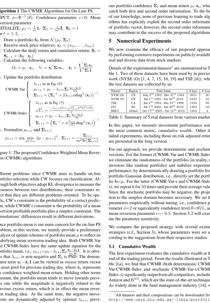
Algorithm 1 The CWMR Algorithms for On-Line PS
INPUT:φ=Φ−1(θ): Confidence parameter; ǫ<0: Mean
reversion parameter
INITIALIZE:µ1=m11, Σ1= m12I, S0= 1 Fort= 1,2, . . .
1: Draw a portfoliobtfromN(µt,Σt)
2: Receive stock price relatives:xt= (xt1, . . . , xtm) 3: Calculate the daily return and cumulative return:St=
St−1×(bt·xt)
4: Calculate the following variables:
Mt=µt·xt, Vt=xt⊤Σtxt, x¯t= 1
⊤Σ
txt
1⊤Σt1 5: Update the portfolio distribution:
CWMR-Var λt+1as in Eq. (5) µt+1=µt−λt+1ΣtxtM−x¯tt1 Σt+1= Σ−t1+ 2λt+1φdiag2(xt) −1 CWMR-Stdev λt+1as in Eq. (7) √ Ut= −λt+1φVt+qλ2 t+1φ 2V2 t+4Vt 2 µt+1=µt−λt+1Σtxt− ¯ xt1 Mt Σt+1= Σ−t1+φ λt+1 √ Utdiag 2 (xt) −1 6: Normalizeµt+1andΣt+1: µt+1= arg min µ∈△mk µ−µt+1k 2 ,Σt+1= Σ t+1 m2Tr(Σ t+1) Figure 1: The proposed Confidence Weighted Mean Rever-sion (CWMR) algorithms.
different problems since CWMR aims to handle on-line portfolio selection while CW focuses on classification. Al-though both objectives adopt KL divergence to measure the closeness between two distributions, their constraints re-flect that they are different problems oriented. To be spe-cific, CW’s constraint is the probability of a correct predic-tion, while CWMR’s constraint is the probability of a mean reversion profitable portfolio plus a simplex constraint. The formulations’ differences result in different derivations. Since portfolio mean is our main concern for the on-line PS problem, in this section, we mainly provide a preliminary analysis of update schemes of portfolio meanµto reflect its underlying mean reversion trading idea. Both CWMR-Var and CWMR-Stdev have the same update equation for the portfolio mean, i.e.,µt+1=µt−λt+1Σt
xt−x¯t1
µt·xt . It is
obvi-ous thatλt+1is non-negative andΣtis PSD. The denom-inator termxt−x¯t1can be viewed as excess return vector of asset pool for previous trading day, wherex¯trepresents the confidence weighted mean return. Holding other terms constant, the portfolio mean tends to move towards previ-ous one while the magnitude is negatively related to the previous excess return, which is in effect the mean rever-sion trading idea. At the same time, the negative move-ments are dynamically adjusted by optimal λt+1,
previ-ous portfolio confidenceΣtand mean returnµt·xt, which catch both first and second order information. To the best of our knowledge, none of previous learning to trade algo-rithms has explicitly exploit the second order information of portfolio vector, however, the second order information may contribute to the success of the proposed algorithms.
5
Numerical Experiments
We now examine the efficacy of our proposed approach by performing extensive experiments on publicly available, real and diverse data from stock markets.
Details of the experimental datasets1are summarized in Ta-ble 1. Two of these datasets have been used by in previous work (NYSE (O) [1, 4, 7, 15, 16, 19] and TSE [4]), while the rest datasets are collected by us.
Dataset Region Time frame # days # Assets NYSE (O) US July3rd
1962- Dec31st
1984 5651 36
NYSE (N) US Jan1st
1985- Jun30th
2010 6431 23
TSE CA Jan4th1994- Dec31st1998 1259 88
STI SG Jan1th
2005- Jun30th
2010 1404 22
MSCI Global Oct17th
2005- Oct15th
2010 1304 4
Table 1: Summary of 5 real datasets from various markets. In this paper, we measure investment performance using the most common metric, cumulative wealth. Other de-tailed experiments, including those on risk adjusted return, are presented in the long version.
For our approach, we provide deterministic and stochastic versions. For the former (CWMR-Var and CWMR-Stdev), we eliminate the randomness of the portfolio (in reality, no investors like random portfolio) and stabilize experiment performance, by deterministically drawing a portfolio from portfolio Gaussian distribution, i.e., directly set the portfo-liob=µ. For the latter (CWMR-Var-s and
CWMR-Stdev-s), we repeat it for50times and provide their average value. Since the stochastic portfolio may be negative, the projec-tion to the simplex domain becomes necessary. We set the parameters empirically without tuning, i.e., confidence pa-rameterφ=2or equivalently confidence levelθ=95%, and mean reversion parameterǫ=−0.5. Section 5.2 will exam-ine the parameter sensitivity.
We compare the proposed strategy with several existing strategies (c.f., Section 3), whose parameters were set ac-cording to the suggestions from their respective studies.
5.1 Cumulative Wealth
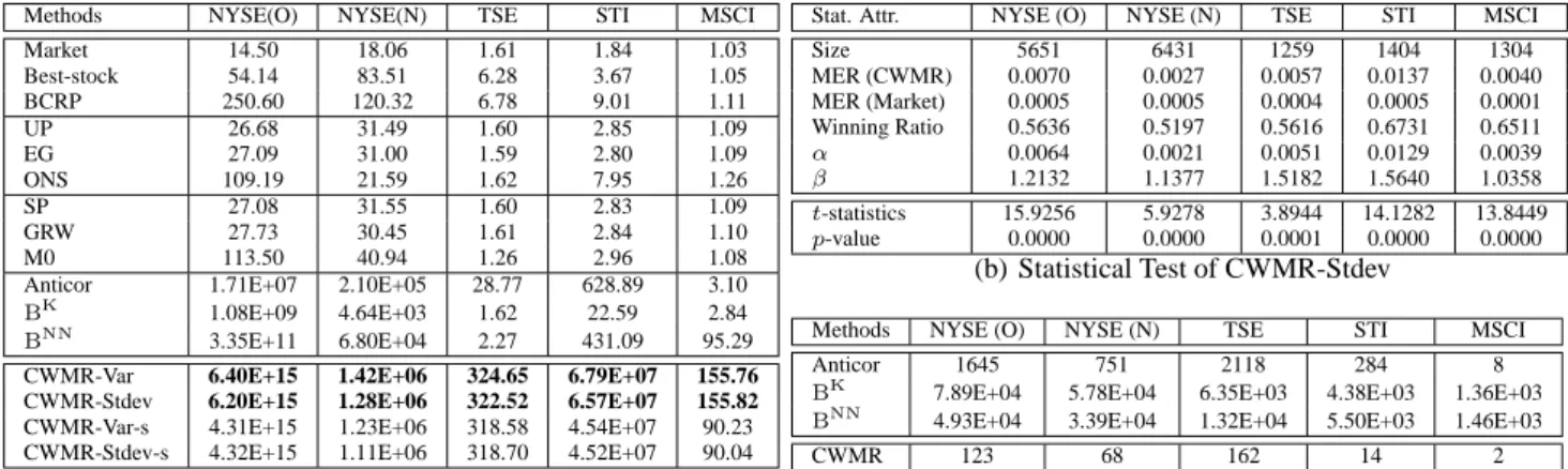
The first experiment evaluates the cumulative wealth at the end of the trading period. From the results illustrated in Ta-ble 2(a), we find that CWMR (both deterministic CWMR-Var/CWMR-Stdev and stochastic CWMR-Var-s/CWMR-Stdev-s) significantly outperform all competitors, including Anticor andBNN, which are the state-of-the-art techniques.
As widely done in the fund management industry [14], we 1
All datasets and their compositions can be downloaded from
also performed statistical tests to examine if the claimed ex-cess return can be generated by simple luck. As the results (Table 2(b)) show, the possibility for achieving the excess return due to simple luck is only0.01%on the TSE dataset and almost0%on other datasets. Finally, we also plot the wealth curve of the cumulative wealth in Figure 3. The figures show that the proposed CWMR algorithm performs consistently over the entire trading period. These results show that the CWMR approach is a promising and reliable PS technique to achieve high return with high confidence.
5.2 Parameter Sensitivity
We now evaluate how different choices of the parameters affect the performance of CWMR. Since confidence pa-rameterφgenerally does not have a decisive influence on the final performance, we evaluate the scalability of the proposed approach with respect to the negative mean re-version sensitivity −ǫ. Figure 4 depicts the results, plus the final cumulative wealth achieved by Market and BCRP strategy for comparison. The figures show clearly that fi-nal cumulative wealth increases as the negative sensitivity grows, and becomes stable as the negative sensitivity ex-ceeds certain critical values, indicating that the power of mean reversion has been thoroughly exploited by our strat-egy. Needless to say, even though our parameter setting, i.e.,−ǫ=0.5, is not the best setting, the proposed CWMR still significantly surpasses existing approaches.
5.3 Practical Issues: Transaction Cost
To evaluate the performance when the market model is not friction-less, we conduct empirical experiments on the proposed CWMR strategy with proportional transaction costs [2, 4]. Figure 5 shows the results on the five datasets with varying transaction costs from0%to1%(we extend x-axis on the STI dataset since the break-even level ex-ceeds1%), plus the cumulative wealth achieved by Market, BCRP and the state of the arts (Anticor andBNN). As we
can observe, the performance with transaction costs is mar-ket dependent, in most cases, especially with small rates, CWMR outperforms the state of the arts. In other cases, though both powered by mean reversion, CWMR underper-forms Anticor, showing that aggressiveness results in more transaction costs. Nevertheless, the results compared with the benchmarks clearly demonstrate that on most datasets (except NYSE (N)), the performance is considerably robust with respect to the transaction costs, where the break-even rates are always above0.6%(around0.2%on NYSE (N)). Thus, CWMR can withstand small transaction costs even though we do not explicitly tackle it in our study.
5.4 Computational Time
Other than the promising cumulative wealth performance, CWMR also runs quite efficiently. Table 2(c) shows the computational time of the CWMR-Stdev and three performance-competing strategies (Anticor,BK andBNN)
on all datasets with the same platform. From the table,
we can observe that CWMR costs much less computa-tional time than the three performance-competing strate-gies, which validates its computational efficiency.
5.5 Discussion and Thread of Validity
Any PS strategy claiming excess returns should be care-fully scrutinized, including CWMR. To recall, we had made several assumptions in Section 2 regarding transac-tion costs, market liquidity, and impact cost, which would affect the practical deployment of the proposed strategy. Ig-noring transaction costs can reduce the problem complex-ity, which is common in existing studies. In Section 5.3, we had examined the effect of varying transaction costs with results showing that CWMR can withstand moderate trans-action costs. The second assumption is that the market is liquid and one can trade any quantity at quoted price. In the experiments, we have tried to minimize the effect of the market liquidity by arbitrary choosing stocks from the market index, which usually have large capitalization and thus have a high market liquidity. The last assumption is that portfolio has no impact to the market. However, as we observed, the portfolio increases astronomically and would inevitably impact the market. In reality, we can reduce the market impact by controlling the size of the portfolio, as typically done by some quantitative funds. Finally, we note again, even in such theoretically “perfect market” typically adopted in previous studies, none has ever claimed such eye-catching performance on the benchmark testbeds. Back tests in the historical market may suffer from “data-snooping bias” issue. In particular, following previous works, in our datasets the composition stocks never delisted from the markets, i.e., survived over the entire trading pe-riod. Another possible “data-snooping bias” is the dataset selection. In fact, we developed CWMR approaches based solely on the widely adopted NYSE (O) dataset, and col-lected other three datasets (NYSE (N), STI, and MSCI) af-ter the algorithm was fully developed.
6
Conclusions
This paper proposed a novel on-line portfolio selection strategy named “Confidence Weighted Mean Reversion” (CWMR), which successfully applied machine learning techniques for on-line portfolio selection by exploiting the mean reversion property of the financial markets. Unlike the existing techniques using only the first order informa-tion, CWMR exploits both the first and second order infor-mation of the portfolio vectors. Empirically CWMR sur-passed all the competing existing techniques on various up-to-date testbeds from real markets. Future work will study theoretical bounds of the logarithmic wealth achieved by CWMR and its performance with high transaction costs.
Acknowledgments
This work was supported by Singapore MOE ARC tier-1 research grant (RG67/07) and tier-2 research grant (T208B2203).
Methods NYSE(O) NYSE(N) TSE STI MSCI Market 14.50 18.06 1.61 1.84 1.03 Best-stock 54.14 83.51 6.28 3.67 1.05 BCRP 250.60 120.32 6.78 9.01 1.11 UP 26.68 31.49 1.60 2.85 1.09 EG 27.09 31.00 1.59 2.80 1.09 ONS 109.19 21.59 1.62 7.95 1.26 SP 27.08 31.55 1.60 2.83 1.09 GRW 27.73 30.45 1.61 2.84 1.10 M0 113.50 40.94 1.26 2.96 1.08
Anticor 1.71E+07 2.10E+05 28.77 628.89 3.10
BK 1.08E+09 4.64E+03 1.62 22.59 2.84
BNN 3.35E+11 6.80E+04 2.27 431.09 95.29
CWMR-Var 6.40E+15 1.42E+06 324.65 6.79E+07 155.76 CWMR-Stdev 6.20E+15 1.28E+06 322.52 6.57E+07 155.82 CWMR-Var-s 4.31E+15 1.23E+06 318.58 4.54E+07 90.23 CWMR-Stdev-s 4.32E+15 1.11E+06 318.70 4.52E+07 90.04
(a) Cumulative Wealth
Stat. Attr. NYSE (O) NYSE (N) TSE STI MSCI
Size 5651 6431 1259 1404 1304 MER (CWMR) 0.0070 0.0027 0.0057 0.0137 0.0040 MER (Market) 0.0005 0.0005 0.0004 0.0005 0.0001 Winning Ratio 0.5636 0.5197 0.5616 0.6731 0.6511 α 0.0064 0.0021 0.0051 0.0129 0.0039 β 1.2132 1.1377 1.5182 1.5640 1.0358 t-statistics 15.9256 5.9278 3.8944 14.1282 13.8449 p-value 0.0000 0.0000 0.0001 0.0000 0.0000
(b) Statistical Test of CWMR-Stdev
Methods NYSE (O) NYSE (N) TSE STI MSCI
Anticor 1645 751 2118 284 8
BK 7.89E+04 5.78E+04 6.35E+03 4.38E+03 1.36E+03 BNN
4.93E+04 3.39E+04 1.32E+04 5.50E+03 1.46E+03
CWMR 123 68 162 14 2
(c) Computational Time (seconds)
Figure 2: Performance evaluation: (a). Cumulative wealth achieved by various trading strategies on the five datasets. The top two best results in each dataset are highlighted in bold font. (b). Statistical t-test of the performance of the CWMR-Stdev on the stock datasets. MER denotes the Mean Excess Return. (c). Computational time costs (seconds) on the five datasets achieved by performance comparable state-of-the-art trading strategies.
100 104 108 1012 1016 1 1500 3000 4500
Total Wealth Achieved
Trading Days CWMR Market BCRP Anticor ΒΝΝ
(a) NYSE (O)
100 103 106
1 1500 3000 4500 6000
Total Wealth Achieved
Trading Days CWMR Market BCRP Anticor ΒΝΝ (b) NYSE (N) 100 101 102 103 1 300 600 900 1200
Total Wealth Achieved
Trading Days CWMR Market BCRP Anticor ΒΝΝ (c) TSE 100 102 104 106 108 1 300 600 900 1200
Total Wealth Achieved
Trading Days CWMR Market BCRP Anticor ΒΝΝ (d) STI 1 10 100 1 300 600 900 1200
Total Wealth Achieved
Trading Days CWMR Market BCRP Anticor ΒΝΝ (e) MSCI
Figure 3: Trend of cumulative wealth achieved by proposed CWMR-Stdev and various strategies during the entire trading period on the stock datasets.
100 104 108 1012 1016 1 2 3
Total Wealth Achieved
-ε CWMR Market BCRP
(a) NYSE (O)
100 103 106
1 2 3
Total Wealth Achieved
-ε CWMR Market BCRP (b) NYSE (N) 100 101 102 103 1 2 3
Total Wealth Achieved
-ε CWMR Market BCRP (c) TSE 100 102 104 106 108 1 2 3
Total Wealth Achieved
-ε CWMR Market BCRP (d) STI 1 10 100 1 2 3
Total Wealth Achieved
-ε CWMR Market BCRP
(e) MSCI
Figure 4: Parameter Sensitivity of the total wealth achieved by CWMR-Stdev with respect to sensitivity parameter−ǫ.
100 104 108 1012 1016 0 0.2 0.4 0.6 0.8 1
Total Wealth Achieved
Transaction Costs (γ%) CWMR Market BCRP Anticor ΒΝΝ
(a) NYSE (O)
100 103 106
0 0.2 0.4 0.6 0.8 1
Total Wealth Achieved
Transaction Costs (γ%) CWMR Market BCRP Anticor ΒΝΝ (b) NYSE (N) 100 101 102 103 0 0.2 0.4 0.6 0.8 1
Total Wealth Achieved
Transaction Costs (γ%) CWMR Market BCRP Anticor ΒΝΝ (c) TSE 100 102 104 106 108 0 0.2 0.4 0.6 0.8 1 1.2 1.4
Total Wealth Achieved
Transaction Costs (γ%) CWMR Market BCRP Anticor ΒΝΝ (d) STI 1 10 100 0 0.2 0.4 0.6 0.8 1
Total Wealth Achieved
Transaction Costs (γ%) CWMR Market BCRP Anticor ΒΝΝ (e) MSCI
Appendix A: Proof of Proposition 1
Proof. First let us replace the log return function
using its first order Taylor expansion at µi, i.e.,
log (µ·xi)≈log (µi·xi) +xi·(µ−µi)
µi·xi . Moreover, since
con-sidering the non-negativity constraint introduces too much complexity, at this stage we solve the problem without con-sidering it, and instead later we will project the solution to simplex domain to obtain the required portfolio.
The Lagrangian for optimization problem (2) is, L=1 2 log detΣi detΣ +Tr Σ−i1Σ + (µi−µ)⊤Σ− 1 i (µi−µ) +λ φx⊤iΣxi+ log (µi·xi) +x i·(µ−µi) µi·xi − ǫ +η(µ·1−1). Taking the gradient of the Lagrangian with respect toµand setting it to zero, we can get the update ofµi+1 :µi+1 =
µi−Σi
λ xi
µi·xi +η
1, whereΣi is assumed to be non-singular. Multiplying both sides of the update with 1⊤, we can get η, i.e., 1 = 1−1⊤Σiλ xi
µi·xi +η
1 ⇒
η = −λ ¯xi
µi·xi, where ¯
xi=1⊤Σixi
1⊤Σi1 denotes the confidence
weighted average of the ith price relative. Plugging η to the update ofµt+1, we can get,µt+1=µi−λΣi
x
i−x¯i1
µi·xi
.
Moreover, calculating the derivative with respect toΣand setting it to zero, we can also have the update ofΣi+1, i.e., Σ−1
i+1=Σ− 1
i +2φλxix⊤i . Thus, the updates forµi+1 and Σi+1are represented as:
µi+1=µi−λΣi xi−xi1¯ µi·xi , Σ−i+1=1 Σ− 1 i +2λφxix⊤i . (4) Now let us solve the Lagrange multiplier λi+1 using the KKT conditions. The inverse of the Σi+1 can also be calculated using Woodbury equation [13], i.e., Σi+1 = Σi−Σixi 2λφ
1+2λφx⊤
iΣixi
x⊤i Σi. The KKT conditions imply that eitherλ=0, and no update is needed, or the constraint in optimization (2) is an equality after the update. Taking Eq. (4) and Woodbury equation to the equality version of the constraint and rearranging the terms, we have:
aλ2+bλ+c= 0, (5) with a = 2φVi2−2φVix¯ix⊤iΣi1 M2 i , b = Vi−¯xix⊤iΣi1 M2 i +
2φVi(ǫ−logMi),c=ǫ−logMi−φVi, andMi =µi·xi is the return mean andVi=x⊤i Σixidenotes the return vari-ance of the ith trading day. Above Eq. (5) is clearly a quadratic equation in λ. We can calculate its roots γi1 and γi2 as follows, γi1=−b+ √ b2−4ac 2a , γi2=−b− √ b2−4ac 2a . To ensure the non-negativity of the Lagrangian multi-plier, we can project the value to [0,+∞), λi+1 =
max{γi1, γi2, 0}.
In practice, since we only adopt the diagonal elements of the covariance matrix, it is equivalent to computingλi+1as Eq. (5) but updating the covariance matrix with the follow-ing rule instead,Σ−1i+1 =Σ−1i + 2λi+1φdiag2(xi), where diag(xi)denotes the diagonal matrix with the elements of xion its main diagonal.
Appendix B: Proof of Proposition 2
Proof. Following the same procedure as the proof of
Proposition 1, we adopt the Taylor expansion of the log function and ignore the non-negativity of the portfolio vec-tor first.
The Lagrangian for the optimization (3) is, L=1 2 log detΥ2i detΥ2 +Tr Υ−i2Υ 2 + (µi−µ)⊤Υ− 2 i (µi−µ) +λ φkΥxik+ log (µi·xi) +xi· (µ−µi) µi·xi − ǫ +η(µ·1−1). Taking the gradient of the Lagrangian with respect to
µ and setting it to zero, we get the update of µi+1,
µi+1=µi−Υ2i
λ xi
µi·xi+η
1, where Υi is non-singular. Multiplying both sides by 1⊤, we get, 1 = 1 − 1⊤Υ2 i λ xi µi·xi +η 1 ⇒ η = − λ¯xi µi·xi, where ¯ xi = 1⊤Υ2 ixi 1⊤Υ2 i1
is the confidence weighted average of ith price relative. Plugging it to the update of µi+1, we get,
µi+1=µi−λΥ2i xi−x¯i1
µi·xi . Moreover, calculating the
deriva-tive of Υ and set it to zero, we also have the update of Υ2 i+1,Υ−2i+1=Υ−2i +λφ xix⊤i √x⊤ iΥ 2 i+1xi
. The two updates can be expressed in terms of the covariance matrix as follows,
µi+1=µi−λΣixi− ¯ xi1 µi·xi , Σ−i+1=1 Σ− 1 i +λφ xix⊤ i p x⊤ iΣi+1xi . (6)
Here,Σi+1is PSD and non-singular.
Now let us solve the Lagrangian multiplier us-ing its KKT condition. We compute the in-verse using Woodbury equation [13], Σi+1 = Σi − Σixi λφ √x⊤ iΣi+1xi+λφx⊤iΣixi x⊤i Σi. Then, letMi=µi·xi,Vi=x⊤i Σixi, andUi=x⊤i Σi+1xi, and multiplying the update ofµi+1byx⊤i (left) andxi(right), we get Ui=Vi−Vi
λφ
√ Ui+Viλφ
Vi which can be solved for Ui to obtain √Ui=−
λViφ+√λ2Vi2φ
2+4V
i
2 . The KKT
condition implies that eitherλ=0, and no update is needed, or the constraint in the optimization problem Eq. (3) is an equality after the update. Substitute Eq. (6) and Woodbury equation to the equality version of the constraint, after rearranging in terms ofλ, we obtain:
aλ2+bλ+c= 0, (7) with a = Vi−¯xix⊤iΣi1 M2 i + Viφ2 2 2 − Vi2φ 4 4 , b = 2 (ǫ−logMi) V i−¯xix⊤iΣi1 M2 i + Viφ2 2 , and
c = (ǫ−logMi)2 − Viφ2. Let γi1 and γi2 be its roots, thus γi1=−b+ √ b2−4ac 2a , γi2=−b− √ b2−4ac 2a . To ensure the non-negativity of the Lagrangian multiplier, we project the value to[0,+∞),λi+1= max{γi1, γi2,0}. Similar to Proposition 1, we can update the diagonal co-variance matrix as,Σ−i+11 =Σ−i1+φλi+1
√ Uidiag
2(x i).
References
[1] A. Agarwal, E. Hazan, S. Kale, and R. E. Schapire. Algorithms for portfolio management based on the newton method. In ICML, pages 9–16, 2006. [2] A. Blum and A. Kalai. Universal portfolios with and
without transaction costs. Machine Learning, 35(3): 193–205, 1999.
[3] A. Borodin, R. El-Yaniv, and V. Gogan. On the com-petitive theory and practice of portfolio selection (ex-tended abstract). In LATIN, pages 173–196, 2000. [4] A. Borodin, R. El-Yaniv, and V. Gogan. Can we learn
to beat the best stock. Journal of Artificial
Intelli-gence Research, 21:579–594, 2004.
[5] S. Boyd and L. Vandenberghe. Convex Optimization. Cambridge University Press, 2004.
[6] L. Breiman. Optimal gambling systems for favor-able games. Proceedings of the Berkeley Symposium
on Mathematical Statistics and Probability, 1:65–78,
1961.
[7] T. M. Cover. Universal portfolios. Mathematical
Fi-nance, 1(1):1–29, 1991.
[8] T. M. Cover and D. H. Gluss. Empirical bayes stock market portfolios. Advances in applied mathematics, 7(2):170–181, 1986.
[9] K. Crammer, O. Dekel, J. Keshet, S. Shalev-Shwartz, and Y. Singer. Online passive-aggressive algorithms.
Journal of Machine Learning Research, 7:551–585,
2006.
[10] K. Crammer, M. Dredze, and F. Pereira. Exact convex confidence-weighted learning. In NIPS, pages 345– 352, 2008.
[11] M. Dredze, K. Crammer, and F. Pereira. Confidence-weighted linear classification. In ICML, pages 264– 271, 2008.
[12] E. J. Elton, M. J. Gruber, S. J. Brown, and W. N. Goetzmann. Modern Portfolio Theory and Investment
Analysis. Wiley, 2006.
[13] G. H. Golub and C. F. Van Loan. Matrix
Computa-tions, 3rd ed. Baltimore, MD: Johns Hopkins, 1996.
[14] R. Grinold and R. Kahn. Active Portfolio
Manage-ment: A Quantitative Approach for Producing Su-perior Returns and Controlling Risk. McGraw-Hill,
1999.
[15] L. Gy ¨orfi, G. Lugosi, and F. Udina. Nonparametric kernel-based sequential investment strategies.
Math-ematical Finance, 16(2):337–357, 2006.
[16] L. Gy ¨orfi, F. Udina, and H. Walk. Nonparametric nearest neighbor based empirical portfolio selection strategies. Statistics and Decisions, 26(2):145–157, 2008.
[17] E. Hazan and S. Kale. On stochastic and worst-case models for investing. In NIPS, pages 709–717, 2009. [18] E. Hazan and C. Seshadhri. Efficient learning algo-rithms for changing environments. In ICML, pages 393–400, 2009.
[19] D. P. Helmbold, R. E. Schapire, Y. Singer, and M. K. Warmuth. On-line portfolio selection using multi-plicative updates. Mathematical Finance, 8(4):325– 347, 1998.
[20] N. Jegadeesh. Evidence of predictable behavior of security returns. Journal of Finance, 45(3):881–98, 1990.
[21] J. Kelly, J. A new interpretation of information rate.
Bell Systems Technical Journal, 35:917–926, 1956.
[22] H. A. Latan´e. Criteria for choice among risky ven-tures. The Journal of Political Economy, 67(2):144– 155, 1959.
[23] T. Levina and G. Shafer. Portfolio selection and on-line learning. International Journal of Uncertainty,
Fuzziness and Knowledge-Based Systems, 16(4):437–
473, 2008.
[24] B. Li, S. C. Hoi, and V. Gopalkrishnan. Corn : Correlation-driven nonparametric learning approach for portfolio selection. ACM Transactions on
Intel-ligent Systems and Technology, 2(3), 2011.
[25] A. W. Lo and A. C. MacKinlay. When are contrarian profits due to stock market overreaction? Review of
Financial Studies, 3(2):175–205, 1990.
[26] H. Markowitz. Portfolio selection. The Journal of
Finance, 7(1):77–91, 1952.
[27] E. Ordentlich and T. M. Cover. On-line portfolio se-lection. In COLT, pages 310–313, 1996.
[28] W. F. Sharpe. A simplified model for portfolio analy-sis. Management Science, 9:277–293, 1963.
[29] W. F. Sharpe. Capital asset prices: A theory of market equilibrium under conditions of risk. The Journal of
Finance, 19(3):425–442, 1964.
[30] Y. Singer. Switching portfolios. International Journal
of Neural Systems, 8(4):488–495, 1997.
[31] E. Thorp. Portfolio choice and the kelly criterion. In
Business and Economics Section of the American Sta-tistical Association, pages 215–224, 1971.
[32] V. G. Vovk. Aggregating strategies. In COLT, pages 371–386, 1990.
[33] V. G. Vovk and C. Watkins. Universal portfolio selec-tion. In COLT, pages 12–23, 1998.