USING REINFORCEMENT LEARNING TO COORDINATE BETTER
CORAB. EXCELENTE-TOLEDO∗
National Laboratory of Advanced Computer Science, LANIA, R´ebsamen No. 80, Col. Isleta, C.P. 91090 Xalapa, Veracruz, Mexico
NICHOLASR. JENNINGS
School of Electronics and Computer Science, University of Southampton, Southampton SO17 1BJ, United Kingdom
This paper examines the potential and the impact of introducing learning capabilities into autonomous agents that make decisions at run-time about which mechanism to exploit to coordinate their activities. Specifically, our motivating hypothesis is that to deal with dynamic and unpredictable environments it is important to have agents that learnthe right situations in which to attempt coordination, andthe right coordination method to use in those situations. In particular, the efficacy of learning is evaluated when agents have varying types and amounts of information when those coordinating decisions are taken. This hypothesis is evaluated empirically, in a grid-world scenario in which (a) an agent’s predictions about the other agents in the environment are approximately correct and (b) an agent cannot correctly predict the others’ behavior. The results presented show when, where and why learning is effective when it comes to making a decision about selecting a coordination mechanism.
Key words:coordination, agent interaction, collaborative agents, reinforcement learning.
1. INTRODUCTION
Effective coordination is essential if autonomous agents are to achieve their goals in a multiagent system (MAS). Such coordination is required to manage the various forms of dependency that naturally occur when the agents have interlinked objectives, when they share a common environment, or when they share resources. To this end, a variety of protocols and structures have been developed to address the coordination problem. These range from long-term social laws (Shoham and Tennenholtz 1992), through medium-term mechanisms such as Partial Global Planning (Durfee and Lesser 1991), organizational structuring (Fox 1981), and market protocols (Malone 1987), to one-shot (short-term) mechanisms such as the Contract-Net Protocol (Smith and Davis 1981).
All of thesecoordination mechanismshave different properties and characteristics and are suited to different types of tasks and environments. They vary in the degree to which coordination is prescribed at design time, the amount of time and effort they require to set up a given coordination episode at run-time, and the degree to which they are likely to be successful and produce coordinated behavior in a given situation. In the majority of cases, these dimensions act as forces in opposing directions; coordination mechanisms that are highly likely to succeed typically have high set up and maintenance costs, whereas mechanisms that have lower set up costs are also more likely to fail. Moreover, a coordination mechanism that works well in a reasonably static environment will often perform poorly in a dynamic and fast changing one. In short, there is no universally best coordination mechanism (Galbraith 1973).
Given this situation, we believe it is important for the agents to have a variety of coor-dination mechanisms, with varying properties, at their disposal so that they can select the particular mechanism that is most appropriate for the task at hand. Thus, for particularly important tasks, the agents may choose to adopt a coordination mechanism that is highly likely to succeed, but which will invariably have a correspondingly large set up cost. Whereas
∗This work was carried out while the first author was a member of the Intelligence, Agents, Multimedia Group at the University of Southampton.
C
for less important tasks, a mechanism that is less likely to succeed, but which has lower set up costs, may be more appropriate. However, to date, the choice of which coordination mechanism to use in a given situation is something that the designer typically imposes upon the system at design time (e.g., in a given application a particular social law will be used or it will be decided that all coordination activities will be handled by the contract net protocol). This means that in many cases the coordination mechanism that is employed is not ideally suited to the agents’ prevailing circumstances. This inflexibility means that the performance of both individual agents and the overall system may be compromised. This is especially the case in open and dynamic environments in which agent-based solutions are often deployed (Jennings 2000).
To rectify this situation, our aim is to develop agents that can reason about the process of coordination and then select mechanisms that are appropriate to their current situation. That is,the choice of coordination mechanism is made at run-time by the agents that need to coordinate. We claim that fixing on a single coordination mechanism at design time is inappropriate, especially in dynamic and open contexts, because there is no scope for changing or modifying the mechanism to ensure there is a good fit with the prevailing circumstances (Bourne, Excelente-Toledo, and Jennings 2000; Excelente-Toledo 2003; Excelente-Toledo and Jennings 2004). To circumvent this problem and to achieve the necessary degree of flexibility in coordination requires an agent to make decisions about when to coordinate and which coordination mechanism to use. To this end, we have previously developed, evaluated and shown the effectiveness of an agent reasoning framework to achieve this (Bourne et al. 2000; Excelente-Toledo 2003; Excelente-Toledo and Jennings 2004). However, this work also highlighted the importance (as well as the difficulty) of making good approximations about the behavior of other agents. This is especially true as the environment becomes more dynamic. Given this, a natural extension of the framework is to enable the agents to acquire knowledge through run-time adaptation. Thus, the agents need to be capable of learning to make the right decisions about their coordination problem.
More specifically, here, we deal with the problem of allowing agents to learn the right situation in which to apply an appropriate coordination mechanism (that has previously been effective in similar circumstances). In particular, we explore the use of a number ofQ-learning algorithms in which the amount of information represented in the state varies. We show how this representation impacts upon the process of making run-time choices about the selection of coordination mechanisms in a number of different scenarios. The reason for this changing state representation is because it models the key determining factors of the agent’s reason-ing framework (i.e., the environmental factors and the responses of the other agents in the group).
This work advances the state of the art in the following ways. Firstly, it introduces learning into that part of the agent’s decision-making process that is concerned with when and how to coordinate (agents learn the right situations in which to attempt coordination and the right coordination method to use in those situations). Secondly, it explores different state represen-tations inQ-learning implementation and, more importantly, it analyzes the efficiency of each in different scenarios regarding coordination decisions. Finally, it empirically demonstrates where the benefits of learning can be obtained and where learning is not beneficial in this decision-making context.
extensions into the agent’s decision-making and examines their impact. Section 7 deals with related work and, finally, Section 8 concludes and presents the areas of further work.
2. THE COORDINATION TESTBED
The testbed domain is described in more detail in (Bourne et al. 2000; Excelente-Toledo 2003) (this includes a detailed justification for the choice of this scenario and the various design decisions within it). Here we just recount the basics that are necessary to understand the subsequent experiments. Our testbed consists of a grid world in which a number of autonomous agents (Ai) perform tasks for which they receive units of reward (Ri). Each
agent has aspecific task(STi) which only it can perform; there are other tasks which require
several agents to perform them, called cooperative tasks (CTs). Each task has a reward associated with it, the rewards for the CTs are higher than those for STs because they must be divided among themcoordinating agents.
The agents move around the grid one step at a time, up, down, left or right, or stay still. At any one time, each agent has a singlegoal, either its ST or a CT over which coordination needs to be achieved. On arrival at a square containing its goal, the agent receives the associated reward. In the case of STs, a new one appears, randomly, somewhere in the grid, visible only to the appropriate agent. In the case of CTs, a new one appears, randomly, somewhere in the grid, but this is only visible to an agent who subsequently arrives at that square. If an agent encounters a CT, while pursuing its current goal (i.e., its ST), it takes charge of the CT1 and must decide on both whether to initiate coordination with other agents over this task, and which coordination mechanism (CM) it should use or continue working on its ST. In this context, each agent has a predefined range of CMs at its disposal. Each CM is parameterized by two types of meta-data (see Excelente-Toledo 2003) for a mapping of several coordination mechanisms into this framework): set up cost (in terms of time-steps) and chance of success. For example, a CM may takettime-steps to set up (modeled by the agent waiting that number of time-steps before requesting bids from other agents) and have a probability,p, of success (thus when the other agent(s) arrive at the CT square, the reward will be allocated with probabilityp, with zero reward otherwise). An agent may well decide that attempting to coordinate is not in its best interests, in which case it adopts the null CM (i.e., the agent rejects adopting the CT as its goal).
The Agent-in-Charge (AiC) of the coordination selects a CM and, after waiting for the set up period, broadcasts a request for other agents to engage in coordination. The other agents respond with bids composed of the amount of reward they would require to participate in the CT and how many time-steps away from the CT square they are situated. If an agent’s bid is successful, then it is termed Agent-in-Cooperation (AiCoop) to denote the fact that it is a participant (not AiC) for a CT task. If however, AiC initiates coordination but there is no AiCoops, then, we say that the AiC failed while attempting coordination. The role Agent-in-ST (AiS) is used to denote the situation where an agent is working towards a ST. Within this broad framework, Figure 1 highlights the specific decisions which have to be made (see Section 3 for more details) and gives the protocol the agents follow at each time-step.
Agents might receive more than one proposal at the same time-step, in which case they reply with as many bids as the proposals they receive. However, they will only accept one CT contract at a time. Agreements between AiCs and AiCoops to achieve a particular CT
1If several agents arrive at a CT square at the same time, one of them is arbitrarily deemed to be in charge and, if an agent
FIGURE1. Basic protocol followed by agents.
are established via a contracting protocol. This Contract-Net-like protocol (Smith and Davis 1981) consists of three steps. In the first step, AiC broadcasts a proposal to all agents. It then waits for the bids. The second step involves selecting the bids and contracts from AiCs and AiS, respectively (evaluation phase). Finally, the third step consists of the commitment about the terms of the contract and the time step at which AiCoops will arrive at the CT square.
This initial presentation involves several simplifying assumptions; in particular com-mon knowledge, a deterministic environment and straightforward coordination mechanisms. However, the framework is also intended to be flexible so that these and other assumptions can be relaxed (see Excelente-Toledo, Bourne, and Jennings 2001) for an example dealing with the dropping of contracts to better exploit new coordination opportunities). To model dynamism, unpredictability and open features in this grid world, the elements in the environ-ment change their values at execution time. Relevant examples include the changing of the tasks’ rewards (both for STs and CTs), the frequency with which tasks appear and disappear in the grid, the number of agents in the environment, and the number of agents needed to achieve a CT. The main consequence of these variations is that they generate an environment in which agents face difficulty in estimating the decisions of other agents. Thus, agents have to make decisions based on factors that cannot be a priori predicted.
3. THE AGENT’S DECISION-MAKING PROCEDURES
In our previous work we have developed and evaluated a decision-making framework for reasoning about whether and how to coordinate in this domain (Bourne et al. 2000; Excelente-Toledo 2003; Excelente-Excelente-Toledo and Jennings 2004) Because the main focus in this paper is on the role and impact of learning on this framework, we do not discuss all the details of the model here. Rather we concentrate on the decisions where learning could have a role to play; that is, which CM to adopt, if any; how much to bid when a request for coordination is received; and how to determine which bid to accept, if any.
the different actions available to it; if it can maintain or improve this rate, it chooses to do so. Of course, this decision model approximates the true relative values of different actions.
3.1. Deciding Which CM to Select
An agent which, while pursuing its current goal, encounters a CT must decide whether to initiate coordination with other agents to perform it. To do this, the agent must determine whether there is any advantage in so doing. This depends not only on the reward that is being offered, but also on the CMs available, as well as on various environmental factors which effect the expected demands of the potential coordinating agents.
To model theexpected demandsof the other agents, the AiC assumes they are randomly distributed throughout the grid, and that their current goals are similarly distributed. Thus, some agents may be near the CT while others may be far away; likewise, for some agents there would be a significant deviation from their ST to reach the CT, while others may be able to coordinate over the CT en route to their own goals. The agent then assesses the possible CMs on the basis of how long before the task can be performed and how much reward it is likely to obtain after deducting the expected reward requirement of the other agents. In the former case, it considers both the set up time and the average distance away each agent is situated, whereas the latter value is based on the amount of time agents must spend deviating to their path and the CM’s probability of success. This assessment determines the amount of surplus reward the agent can expect, over and above what it expects to obtain during its normal course of operation (i.e., its own average reward per time-step,r). The agent then selects the CM that maximizes this surplus.2
To formalize this decision procedure, consider an [M×N] grid with reward sizeS for STs, andRfor CTs, a coordination mechanism, CMj =(tj, pj), which coststtime-steps to
set up and has a probability of successp. In this grid world of known size, the agent can calculate the expected average distance (ave dist) away of any randomly situated agent from the CT square as well as the likely average deviation (ave dev) such agents would have to make to get there.
Based on these figures, the agent can assess the average surplus reward from coordinating over the CT at (x, y) using CMj =(tj, pj). First, it must estimate its own cost in terms of
how long the CM will take to set up and how long it expects to wait for the other agents to arrive. Because the AiC would usually expect to receiveS reward units per time-step, the average is calculated asr = ave distS . The cost of CMj is then given by:
costj(x,y)=r ×(tj+ave dist(x,y)).
Second, the AiC must estimate the average amount of reward the otherm agents will require. When AiC does not have any knowledge of the average reward of all the other agents in the environment, it uses its own (r) average reward as an approximation.3
ave bidj(x, y)=m×
r×ave dev(x, y)
pj
. (1)
2Though this may not be a globally optimal criterion for deciding which CM to use, it makes sense from a self-interested
agent’s point of view.
3To estimate (1) it is assumed that the m is determined in advance or is part of the agent’s knowledge. However, this
FIGURE2. Example of a coordination world grid.
Third, the AiC estimates the expected surplus (ave payoff) of CMj from adopting the
CT by taking into account the probability of success of the task:
ave payoffj(x,y)= pj ×R
Using these estimates, the AiC can evaluate the expected surplus reward of adopting CMj:
ave surplusj(x,y)=ave payoffj(x,y)−costj(x,y)+ave bidj(x,y). (2)
When deciding which of its CMs to adopt, the agent computes its expected surplus reward from each of them and selects the one that maximizes this value. If the surplus associated with all CMs is negative, the agent adopts the option of the null CM (which is defined to have zero surplus).
To exemplify this decision procedure, consider the simple scenario of Figure 2 at one instant in time with two agents (AiS1and AiS2), two STs, one CT and two CMs : CM1(3, 0.9)
and CM2(6, 1.0). AiS2occupies a [5×5] grid and finds a CT requiring one other agent with R=6 at square [3, 2]. The average distance of other agents from [3, 2] is 2.6. Because the average distance between two random squares is 3.2, the average deviation of any agent from [3, 2] is 2. Assume that each ST has a rewardS =2, then the average reward per time-step of all agents is 32.2 =0.625. The expected surplus reward of adopting each CM is given by:
cost1(3, 2)=(0.625×(3+2.6))=3.5
ave bid1(3, 2)=
(0.625×1×2)
0.9 =1.389 ave payoff1(3, 2)=(0.9×6)=5.4
ave surplus1(3, 2)=0.511
cost2(3, 2)=(0.625×(6+2.6))=5.375
ave bid2(3, 2)=
(0.625×1×2)
1.0 =1.25 ave payoff2(3, 2)=(1.0×6)=6
ave surplus2(3, 2)= −0.625.
Under these circumstances, AiS2decides to attempt coordination with CM1(becoming
negative result indicates there is not likely to be a surplus. Thus, in this case, if AiS2 only
had CM2 at its disposal it would choose the null CM (expected surplus zero) and it would
continue towards its ST.
3.2. Deciding What to Bid to Become an AiCoop
When agents receive a request to participate in a CT they submit a bid based on the amount of reward that they would require to compensate them for deviating from their current goal. Thus, an agent’s required reward is determined by the amount of time spent in deviating to the CT square, its average reward per time-step and the probability of success of the CM being proposed.4
To formalize this, consider an agent, Ai, with average reward per time-stepri. The agent
calculates itsdeviation(i.e., the number of extra time-steps it requires to reach its ST if it goes via the CT square). Note that if, for example, the CT square lies directly on a path to the ST, the agent’s deviation would be zero. Clearly, such an agent will be in a position to submit a very attractive bid, because the cost of coordinating is effectively zero.
Again by means of illustration consider the agents depicted in Figure 2. AiS1at [5, 3]
would take four time-steps to reach ST1at [2, 4] directly, but six steps going via the CT at
[3, 2], a deviation of two time-steps. However, AiS2at [1, 1] would take seven time-steps to
reach ST2at [4, 5] directly, and also seven steps going via the CT at [3, 2]; AiS2, therefore,
has a deviation of 0.
To compute the reward AiSirequires from engaging in coordination over the CT, it takes
into account the compensation both for its deviation and for the possibility that the CM might fail. Thus, the estimation ofbidby agentito participate in coordination is given by:
bidi j =
ri ×deviationi
pj
. (3)
The agent submits its bid to coordinate and its distance from the CT square. If an agent is selected to coordinate, it adopts the CT as its current goal. Its ST is only readopted after the CT has been accomplished.
3.3. Deciding Which AiS Bids to Accept
Once the AiC has received bids from all agents, it selects the set that maximizes its surplus reward, given the new (definite) information it has received (see the approximation in Section 3.1). For each agent, Ai, the AiC knows the amount of reward it will require (bidi j)
and the time it will take to arrive (Ti).
The AiC’s selection bid process is based on the calculation of the cost of each bid received. However, when more than two agents are required to achieve a CT, it is necessary to deal with the fact that an AiCoop may have to wait in the CT cell while the remaining AiCoops arrive (because agents have to travel different distances). There are many ways of dealing with this situation (see discussion below). However, to simplify the estimates of expected reward undertaken by the various agents, it is assumed the AiC pays an additional reward for the time elapsed. Thus, AiC knows the number of time-steps that each AiCoop is likely to have to wait (specified in the bid) and the amount it will pay for waiting time at a specific predefined waiting rate (q). The CT is achieved only when the AiC has received the confirmation of all
4Note that the AiSs use the actual values of the concepts discussed, whereas the AiC’s task is to make a good approximation
magents involved in the cooperation. When an AiCoop notifies the AiC of its arrival at the CT cell, it either receives its share of the CT reward or the waiting rate followed by its share of the CT reward.
Thus, to decide which bids to accept, the general idea is that AiC selects themproposals with least cost (from the total bids receivedB). It does this by considering the reward requested in the bid and the waiting time cost (cost bid) and then it estimates its expected reward given this cost and its investment. Formally, AiC calculates the cost of each subsetbofBwithm
elements of the form (bidi j,Ti). From each subsetb, AiC selects the agent that will take the
longest time to arrive (i.e.,max Tb=max(bidi j,Ti)∈b[Ti]), then it can determine the maximum time that each agent will spend in the cell. Finally, it approximates the cost of each bid based on the reward and the waiting time an AiC has to pay:
cost bidb=
(bidi j,Ti)
(bidi j +(max Tb−Ti)×q).
Bringing all this together, AiC estimates the surplus it expects to obtain by taking into account the cost of the selected bids and its own investment to wait for the last AiCoop to arrive. The bids selected belong to the subsetbofBthat maximizes thesurplusgiven by:
surplusj = pj ×R−cost bidb−r ×(tj +max Tb). (4)
Now, it may be the case that no bids are received that give a positive surplus. Even though the chosen CM had an expected surplus, by chance it may be that no agents are sufficiently near to provide reasonable bids. In such a situation, the AiC abandons the CT and returns to its ST.
In this paper, the main focus is on giving the agents the capability of learning to make the right decisions about their coordination problem. That is, we wish to endow the agents with the capability of learning the right situation in which to apply the right coordina-tion mechanism. Specifically, the agent’s decision-making framework presented in this sec-tion and, in particular, the decision procedure outlined in Secsec-tion 3.1 (equasec-tion (2)), allows agents to make decisions about when and which CM to select to achieve a CT. Thus, this is the major one with respect to reasoning about coordination mechanisms (Bourne et al. 2000; Excelente-Toledo 2003; Excelente-Toledo and Jennings 2004) and it is, therefore, the one we concentrate on in terms of evaluating the role of learning as described in the next section.5
4. THE ROLE OF LEARNING
Our investigation focuses on the use of reinforcement learning (RL) (Kaelbling, Littman, and Moore 1996; Sutton and Barto 1998) in coordination. A reinforcement-based approach is appropriate because we are concerned with agents pursuing goals and obtaining rewards according to how effectively those goals are accomplished. Within this class, Q-learning (Watkins and Dayan 1992) was chosen because it is an online algorithm that does not require a model of the environment and, thus, it is well suited to our dynamic and unpredictable scenario.
5There are other places where learning could play a role; for example, an agent might learn the decision about how much
In this study, each RL agent uses aQ-learning algorithm. In general terms, an agent’s objective is to learn a decision policy that is determined by the state/action value function. The classical model ofQ-learning consists of:
r A finite setSof statessof the world (s∈S);
r A finite setAof actionsathat can be performed (a∈A); r A reward functionR:S×A→r.
An agent’s goal consists of learning a policyπ :S→A that maximizes the expected sum of discounted rewardsV:
Vrt +γrt+1+γ2rt+2+ · · ·
=V
∞
i=0
γir t+i,
where 0≤γ < 1 is the discount factor. Formally speaking, the discount factor determines the value of future rewards in the following way: a reward r received t time-steps in the future is worth onlyγt times what it would be worth if it were received immediately. As
γ approximates 1, the function takes future rewards into account more strongly. Thus, the agent’s task is to learn the optimal policyπ(i.e., arg maxπVπ(s),∀(s)).
In more detail, assume that an agent always performs the cycle of being in a particular states, then selecting and performing an actionathat causes the agent to enter a new state s and receive an immediate payoff (rewardr(s,a)). TheQ-learning algorithm is based on the estimated values of the agent’s state (s)-action (a) pairs, calledQ(s,a) values. Based on this experience, the agent updates itsQ(s,a) values using the formula:
Q(s,a)←Q(s,a)+αr+γ ×max
a Q(s
,a)−Q(s,a), (5)
where α is the learning rate which determines the rate of change of the estimation and, maxaQ(s,a) is the value of the action that maximizes theQfunction at states.
However, there is still the problem of how agents select their next action to execute. They have to balance their decision between selecting an action that, when exploited in the past, brought about a positive reward, and an action that has not yet been explored and that consequently has an unknown reward (“exploitation versus exploration”) (Sutton and Barto 1998). In this work, we use a-greedy function that selects the action with the highestQ(s,a) value once all the actions have been explored a predetermined number of times. In particular, we use f(Q(s,a),n) (Russell and Norvig 1995) which determines how greed (preference for high values ofQ(s,a)) is traded off against curiosity (preference for low values ofn, namely, actions that have not been tried before). Formally speaking, the exploration function equates to:
f(Q(s,a),n) =
R+ ifn < Ne
Q(s,a) otherwise , (6)
wherenis the number of timesQ(s,a) has been visited,R+is the optimistic estimate of best possible reward that an agent can obtain in a given state andNecorresponds to the number
of times that agents should try a particular action-state pair.
of times aQ(s,a) value is visitedα = 1+visits1 (s,a); theQ(s,a) values are initialized with 0. And equation (6) is used as the exploration function.6
Thus, the main objective is then to evaluate the effect of learning on the agents’ decision making about CMs. To do this, we will compare the performance of agents that use a Q-learning algorithm (RL) with those that perform no Q-learning (NL). Here the key difference is how the agents select the CM with which they will attempt coordination (step [2] in the protocol specified in Figure 1). For the remaining steps of the protocol, both RL andNL agents employ the decision-making procedures outlined in Section 3 to make agreements whensurplus(equation (4)) is positive given the set ofbids (equation (3)) it received.
This means then that when dealing with RLagents, the agent-state corresponds to the abstraction of the particular situation that agents experience when a CT is found (e.g., the agent role and the position in the grid); the agent-action represents the set of options an agent has at its disposal (i.e., the set of coordination mechanisms it can select, including the null CM) and the reinforcement is modeled as the reward obtained by selecting the particular CM or not selecting a CM at all. Thus, the idea is that withQ-learning the agents will eventually learn the policy (after exploring sufficient situations) that allows them to know which CM to choose given a specific situation/state.
Now, for the purposes of this analysis, NL and RL agents experience one of the the following outcomes: (i) a successful coordination (i.e., the AiC selects a CM, finds AiCoops to coordinate with and the CT is successfully achieved using the CM selected); (ii) the AiC initiates coordination with a selected CM but there are not enough successful bids to make agreements (this means that attempting coordination with the CM was a failure); and (iii) the AiC does not select any of the CMs at its disposal (i.e., the null CM is selected and the agent continues with its individual problem solving activity).
On the basis of previous description, the learning agent’s main objective is then to select the most suitable CM given its prevailing circumstances. To achieve this general goal, we explore the use of twoQ-learning algorithms:RL1 andRL2. The main difference between them is in the way they model the state representation at the moment when the decision about which CM to select is taken. In particular, our interest is in evaluating whether agents can improve their performance by explicitly representing one of the key components of the decision making of the CM, namely theave bid(equation (1)).7Thus,RL2 agents employ
aQ-learning algorithm that does estimate and useave bidwhen selecting the CM, whereas RL1 does not model this information in its state representation.
Thus, in what follows, we first describe the general RL algorithm and then we detail the differences betweenRL1 andRL2. Finally, we discuss the algorithm followed by theNL agents.
RL:When a learning agent finds the CT, it performs the following basic cycle: 1. It is in a particular state (represented bys)
2. It makes a decision about the next action (a) to execute using the exploitation and exploration function of equation (6).
3. The agent executes the selected action (a) which will be one of accomplishing a CT (if a CM is selected and successful), failing on a CT (if a CM is selected and unsuccessful), or selecting no CM (if the null CM is selected) and reaches a new states.
6It is well known that the convergence time is determined by the exploitation and exploration function, the size of the
look up table and the learning rate (Singh et al. 2000). Here, it was not our objective to hand tune all these parameters to reduce the convergence time in particular cases. Rather, we fixed the values of all parameters and kept them constant in allQ-learning implementations.
4. It obtains a reinforcement reward as a result of the execution of actiona. In particular, the reinforcement varies with the following outcomes:
• The CT is accomplished using the CM selected. In this case, a positive reinforcement is obtained that is based on the reward gained by achieving the CT after the payment to theAiCoops and the time invested in pursuing the task.
• The CT failed given the CM chosen. This situation occurs because no one replies to the request for coordination or because the reward requested to participate in the cooperative action by theAiCoops is too high for the AiC to accept it (i.e., thesurplus (equation (4)) is negative). In either case, a negative reinforcement is calculated based on the average reward (r) lost in the time invested in the CM (t).
• The null CM is explored or exploited. Here, the reinforcement corresponds to the reward (CT reward) the agent might have obtained by investing an average time in a CT (modeled by average distanceave dist).
5. It updates theQ(s,a) value (equation (5)). 6. It goes to [1].
Turning now to the differences between the learning agents and taking previous descrip-tions of RL we have two variations: RL1 and RL2 agents. Each of them will be dealt in turn.
• RL1: An agent learns to select a CM by exactly following the RL algorithm and, in particular, it uses its role and position in the grid when the CT is found as the representation ofs.
• RL2:An agent learns to select a CM usingave bid. An agent of this type followsRLbut has a modified state representationsand a different means of updating tosin step [4]. Specifically,sis modeled with the agent’s role, its position in the grid and the expected ave bid.8The initial estimation ofave bidin step [1] corresponds to:
ave bidj(x, y)=m×r ×ave dev(x,y).
Note that the only difference between this formulation and equation (1), is that pj (the
probability of success of a given CM) is unknown at this stage.
When RL2 agent reaches a new states, the state is updated with the ave bidusing equation (1) wherepj refers to the probability of success of the CM chosen.
NL:A nonlearning agent makes decisions entirely based on the decision-making procedures detailed in Section 3 and follows the protocol specified in Figure 1. Being precise, when an agent finds a CT, it calculates the expected average surplus (equation (2)) of each CM at its disposal. It then simply chooses the one with the bestave surplus. For the next stages of the protocol, it uses equations (4) to decide which bids to accept and (3) to becomeAiCoop. Note that theNLagent uses equation (1) to calculateave bidto evaluateave surplusfor each of the CMs.
To finish the discussion on the role of learning in this model, it is necessary to specify the features of the environment in which the algorithms will be tested. Two scenarios have been designed:scenario1 in which all AiSs in the environment become AiCoop by submitting
8To simplify the state representation,ave bidis in fact associated with a range of values. Given the values of the simulation
variables (see Section 5.1), the ranges of theave bidare the following: 1<ave bid<1.84, 1.84≥ave bid<2.64 and
a bid which is calculated by equation (3) andscenario2 in which AiSs calculate their bids in the same way but they vary the result by a random factor. The reason for this change is that, in the general case, AiCs face a great deal of uncertainty in predicting this value. Thus, the random element mirrors environments in which predictions are less accurate. Together, these two scenarios constitute a reasonably static environment in which good predictions can be made and a more dynamic one in which predictions are inherently less accurate.
Bringing this all together, the agents’ performance will be analyzed using the following algorithms:
RL1 agents learn to select a particular CM according to the profit gained by accomplishing CTs with a particular CM.
RL2 agents learn to select a particular CM according to the accuracy with which they calculate theave bid.
NLagents select a particular CM using equation (2).
5. EVALUATION METHODOLOGY
The main hypothesis we seek to evaluate is whether agents coordinate more effectively in our scenario using the reinforcement-based algorithms. To measure such benefits in our model, a set of experiments have been designed as a formal methodology to provide infor-mation about the experimental variables. To test and to verify the hypothesis questions we employ statistical inference methods; in particular analysis of variance (ANOVA) is used to test hypotheses about differences between the means collected. The null hypothesis (H0) of equal means can be rejected when the procedure reveals for all experiments that the differences among means are significant (p < 0.05) or might be accepted in the contrary case (Cohen 1995). In other words, ANOVA tests the significance of the observations by accepting or rejecting the hypothesis formulated. The observations are the set of values for the experimental variables as the result of the execution of a particular algorithm in a given environment.
ANOVA explains the relationships between groups by analyzing all possible interactions among them. However, though it provides an answer to the hypothetical questions by indi-cating if the mean of the groups are equal or not, it does not indicate the relations between them (e.g., which mean of which groups are the highest). Thus, in most cases, it is neces-sary to go a step further (postanalysis) to determine where the exact differences among the means occur between groups. This procedure consists of running a posttest to explore the data collected on a case by case basis (this is termed pairwise analysis) because it tests the difference between each pair of means.9This pairwise analysis is particularly important in those cases where more than two procedures are being tested (or one procedure is tested in more than two scenarios). In concrete terms, the posttest makes a comparison between the data collected and builds groups (as many as necessary) that have statistically homogeneous values. Each group is generated with an associated value (the p value) that indicates the degree of confidence from which each group was built.
For the purposes of the experimental evaluation presented in Section 6, all the hypotheses are evaluated with ANOVA and only the cases that involve more than two experimental variables are subject to a post evaluation. When we test two variables and ANOVA rejects
9Several statistical tests exist to perform this analysis. The one used here is called Tukey’s honestly significant difference
the equality of means, the data collected is used to indicate the relationship between the two variables. We are also interested in determining which of the groups obtains the highest mean (from now on referred to as thewinner group) because it represents the agents with the best performance.
5.1. Experimental and Simulation Variables
The following simulation variables were fixed for all learning experiments: size of the grid ([10×10]), duration (500,000 time units),10number of CTs in the grid at any one time (3), number of agents in the environment (5), ST reward (1), CT reward (20), maximum number of agents needed to achieve a CT (3), coordination mechanisms considered by an agent (CM1=
(1, 0.6), CM2=(15, 0.7), CM3=(30, 0.8), CM4 =(45, 0.9) and CM5=(60, 1.0)).11
The experimental variables on which the analysis is based are: total agent reward obtained from its ST and CT tasks (AU), total agent reward obtained by agents in the Agent-in-ST role (AiS), total agent reward obtained by agents in the Agent-in-Charge role (AiC), total agent reward obtained by agents in the Agent-in-Cooperation role (AiCoop) and, the total number of CTs accomplished (TCT). The experiments described collect the results of the experimental variables averaged over 10 simulation runs.
5.2. Evaluating Hypotheses
To accept our main hypothesis, the hypotheses presented below must be rejected (meaning that the hypothesis of equal means is false) and the values of the experimental variables of a particular learning algorithm should produce significantly better results than those obtained withNL. Therefore, the following hypotheses must be tested inscenario1 andscenario2:
H1: TheAUobtained by performing a reinforcement-based algorithm (RL) is the same as that obtained by agents which use theNLalgorithm.
H2: The number of CTs (TCT) achieved by agents by means of either RL algorithm is identical to that of agents usingNL.
H3: TheAUobtained byRL1 is the same as that ofRL2 (evaluated in the case where H1 rejected).
H4: The number of CTs accomplished byRL1 is identical to that ofRL2 (evaluated in the case where H2 is rejected).
6. EXPERIMENTAL EVALUATION
The experimental evaluation undertaken in this section follows the methodology de-scribed previously and is organised in the following way. Firstly, the four hypotheses of Section 5.2 are tested in a static environment (Section 6.1) and secondly the same evaluation procedure is followed but in a dynamic environment (Section 6.2).
10We decided to evaluate over a fixed duration because in this scenario time counts and agents win reward at each time-step.
Thus, it is reasonable to compare the behavior of all algorithms under the same parameters. The duration selected is sufficient for the learning algorithms to converge to optimal values.
11These CMs were selected because previous results have indicated that these are the main ones that are selected by the
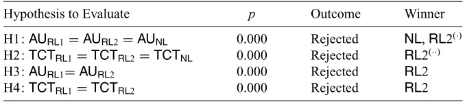
TABLE1. Agent’sAUandTCTinScenario1
Hypothesis to Evaluate p Outcome Winner
H1:AURL1=AURL2=AUNL 0.000 Rejected NL,RL2(·)
H2:TCTRL1=TCTRL2=TCTNL 0.000 Rejected RL2(··)
H3:AURL1=AURL2 0.000 Rejected RL2
H4:TCTRL1=TCTRL2 0.000 Rejected RL2
(·)See Table 2 and(··)Table 3 for details.
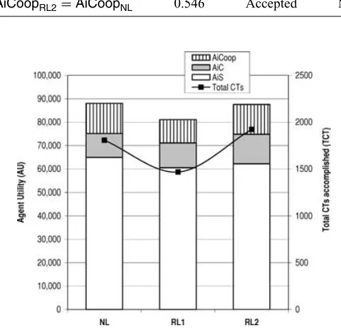
FIGURE3. Contrasting agent’s abilities inscenario1.
6.1. Selecting CMs in Static Environments (scenario1)
To start with, Table 1 and Figure 3 present a summary of the results obtained by per-forming ANOVA on the data collected by each of the algorithms in scenario1. Let us first analyze the agent utility hypothesis. H1 is rejected, meaning that the performance of the algorithms does have a significant effect on the AU obtained. To understand the relationship between the algorithms a postanalysis of H1 is conducted (Table 2). The conclusion is that the performance of NL and RL2 is better by a statistically significant amount (AUNL=88,018.64,AURL2=87,570.24) thanRL1(AURL1=81,064.28).
Further-more, comparing the performance ofRL1 andRL2 in H3 (Rejected), it is concluded that the different mechanisms used for learning do effect theAUobtained by agents. Figure 3 graphi-cally shows that the reward gained byRL2 agents is better than that forRL1 agents. Moreover, it can also be concluded that an agent which learns to select the CM (RL2) performs the same as one which does not learn at all (NL).
[image:14.504.84.423.69.144.2] [image:14.504.140.369.170.376.2]TABLE2. H1 inscenario1: Postanalysis
Agent AU
1 2
RL1 81,064.28
RL2 87,570.24
NL 88,018.64
p 1.000 0.791
TABLE3. H2 inscenario1: Postanalysis
Agent TCT
1 2 3
RL1 1465.62
NL 1805.90
RL2 1922.20
p 1.000 1.000 1.000
TABLE4. ContrastingRL2 andNLAgents inscenario1
Hypothesis to Evaluate p Outcome Winner
H5:AURL2=AUNL 0.594 Accepted None
H6:TCTRL2=TCTNL 0.000 Rejected RL2
this is an important result to analyze in detail, because a high number of CTs achieved, does not necessarily mean that an agent performs better. This argument can be seen by observing Tables 2 and 3 (Figure 3 graphically shows the same information). Here, despite the fact that RL2 agents achieved statistically the highest number ofTCT(three groups were formed in the postanalysis), theirAUgained is not higher than that obtained byNLagents (RL2 and NLagents belong to the same group in Table 2). Actually, the results of applying ANOVA to theTCTachieved andAU gained byNLandRL2 corroborate this explanation and are shown in Table 4. Specifically, H5 shows that the total reward obtained byRL2 is the same as that obtained by agents using theNLalgorithm (H5 is accepted, there is no statistically significant effect on theAU), whereas H6 demonstrates that the total number of CTs achieved byNLagents is identical to theTCTs accomplished byRL2 agents (H6 is rejected, theTCT obtained by each algorithm is significantly different).
TABLE5. ContrastingRL2 andNLAgent’s roleAUinscenario1
Hypothesis to Evaluate p Outcome Winner
H7:AiSRL2=AiSNL 0.009 Rejected NL
H8:AiCRL2=AiCNL 0.000 Rejected RL2
H9:AiCoopRL2=AiCoopNL 0.546 Accepted None
FIGURE4. Contrasting agent’s roles abilities inscenario1.
H7: TheAUobtained by Agents-in-ST role, which perform a reinforcement-based algo-rithm (RL2) is the same as that obtained byAiSagents which use theNLalgorithm. H8: The total reward obtained byRL2 agents in theAiCis the same as that obtained byNL
AiCagents.
H9: TheAUobtained byRL2 Agents-in-Cooperation role (AiCoop) is identical to the total reward obtained byNLagents in theAiCooprole.
Figure 4 illustrates these results. They indicates that while RL2 AiC is significantly better than the correspondingNLagent role (H8 rejected),NL AiSis better thanRL2 AiS (H7 rejected). H9 is accepted which means that the two agents accomplish similar rewards in theirAiCooprole. As can be seen, both agent types achieve (statistically speaking) the same AU (recall that H5 was accepted) but from different sources. In this experiment, the best AiC(as a result of accomplishing more CTs) does not mean more reward is obtained. This is because highAUmight have originated from fewer and more profitable CTs (in the case ofNL) or a high number of less rewarding tasks (in the case ofRL2). In terms of selection of the CMs, this means thatNLselected those with higher probability of success and higher time to set up (less time to achieve CTs), whileRL2 agents choose those CMs with less time to set up but less probability of success.
[image:16.504.104.405.73.133.2] [image:16.504.127.376.119.360.2]TABLE6. Agent’s RoleAUinscenario1
Hypothesis to Evaluate p Outcome Winner
H10:AiSRL1=AiSRL2=AiSNL 0.000 Rejected NL(·)
H11:AiCRL1=AiCRL2=AiCNL 0.000 Rejected RL2(··)
H12:AiCoopRL1=AiCoopRL2=AiCoopNL 0.000 Rejected NL,RL2(···)
(·)See Table 7,(··)Table 8, and(···)Table 9 for details.
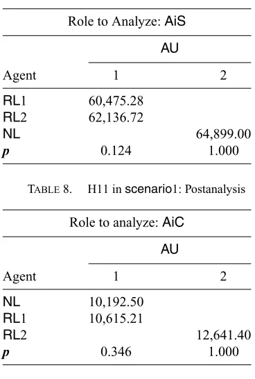
TABLE7. H10 inscenario1: Postanalysis
Role to Analyze:AiS
AU
Agent 1 2
RL1 60,475.28
RL2 62,136.72
NL 64,899.00
p 0.124 1.000
TABLE8. H11 inscenario1: Postanalysis
Role to analyze:AiC
AU
Agent 1 2
NL 10,192.50
RL1 10,615.21
RL2 12,641.40
[image:17.504.70.430.70.132.2]p 0.346 1.000
Figure 4 show the result of the data collected and Tables 7, 8, and 9 present the postanalysis performed to H10, H11 and H12, respectively.
H10: TheAUobtained by Agents-in-ST role which perform a reinforcement-based algo-rithm (eitherRL1 orRL2) is the same as that obtained byAiSagents which use the NLalgorithm.
H11: The total reward obtained byRL1 and RL2 agents in AiC role is the same as that obtained byNL AiCagents.
H12: TheAU obtained byRLs Agents-in-Cooperation role (AiCoop) is identical to the total reward obtained byNLagents in theAiCooprole.
[image:17.504.158.342.172.445.2] [image:17.504.162.338.323.435.2]TABLE9. H12 inscenario1: Postanalysis
Role to analyze:AiCoop
AU
Agent 1 2
RL1 9973.79
RL2 12,792.12
NL 12,927.13
p 1.000 0.746
cooperative activity (H10 rejected)). Turning to the analysis of the cooperative behavior, here the results of Table 5 show thatRL2 is the agent which performs the best as anAiC(H11 is rejected) and (RL2 andNL) obtain the same as anAiCoop(H12 is rejected as both agents have statistically speaking the same results). Generally speaking, it can be seen thatRL2 and NLbetter balance their decision of when to go for the CT with the CM, which allows them to gain more reward.
When considering the two learning-based algorithms, it is clear that those agents that take into account theave bidof other agents (RL2) perform better than those that do not (RL1). Thus, H3 and H4 are rejected in Table 1 and RL2 is the winner in both cases. Moreover, the information provided by the policies learnt by RL2 is more informative. For example, both agents learn that the optimal action when agents are in the corner of the grid (position [1,10]) is to select CM1. However, withRL2, agents additionally learn that this is the action to
execute if and only if theave bidis higher than 2.64. Generally speaking, the optimal policy withRL2 might vary for each of the different values of theave bid, whereas withRL1 this information cannot be extracted from the policies because it is not explicitly represented.
TABLE10. Agent’sAUandTCTinscenario2
Hypothesis to Evaluate p Outcome Winner
H1:AURL1=AURL2=AUNL 0.000 Rejected RL2(·)
H2:TCTRL1=TCTRL2=TCTNL 0.000 Rejected NL(··)
H3:AURL1=AURL2 0.000 Rejected RL2
H4:TCTRL1=TCTRL2 0.200 Accepted None
(·)See Table 11 and(··)Table 12 for details.
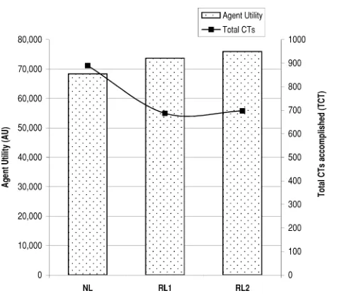
FIGURE5. Contrasting agent’s abilities inscenario2.
accurately predict the other’s behavior and it is very unlikely that agents can successfully use the same decision-making framework. Thus, for these reasons, we believe our agents should be capable of adapting their decision making as a result of what is occurring in the environment, that is, during acting in more demanding scenarios. Therefore, our objective is to design agents that inhabit open and dynamic environments and we require the learning agents to show a superior performance when considering both the exploring and the exploiting phases. Thus, in what follows, the use of learning is further explored in situations in which one of the fundamental actions associated with cooperative activity is more challenging to predict (scenario2).
6.2. Selecting CMs in Dynamic Environments (scenario2)
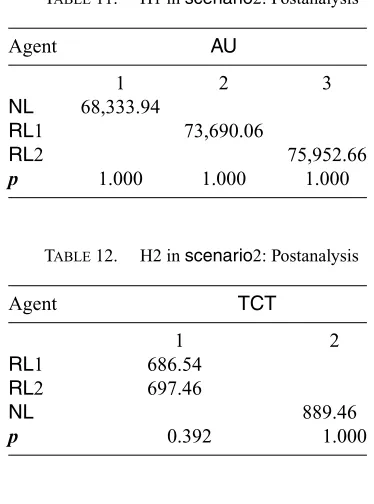
Turning now to the more dynamic environment ofscenario2. We tested the same basic set of hypotheses (H1, H2, H3, and H4) and the results are summarized in Table 10 and Figure 5. First, we analyzed the hypotheses related withAU. Similar to the results obtained in Table 1, we conclude that applying RLs andNLproduces distinctive results. However, conversely to Table 1,RL2 agents get significantly better results (AURL2=75,952.66) than
RL1 agents (AURL1 =73,690.06) and RL1 agents get a significantly higher AU than NL
[image:19.504.101.402.71.145.2] [image:19.504.134.372.163.374.2]TABLE11. H1 inscenario2: Postanalysis
Agent AU
1 2 3
NL 68,333.94
RL1 73,690.06
RL2 75,952.66
p 1.000 1.000 1.000
TABLE12. H2 inscenario2: Postanalysis
Agent TCT
1 2
RL1 686.54
RL2 697.46
NL 889.46
p 0.392 1.000
TABLE13. Agent’s RoleAUinscenario2.
Hypothesis to Evaluate p Outcome Winner
H10:AiSRL1=AiSRL2=AiSNL 0.000 Rejected RL2(·)
H11:AiCRL1=AiCRL2=AiCNL 0.000 Rejected NL(·)
H12:AiCoopRL1=AiCoopRL2=AiCoopNL 0.000 Rejected NL (···)
(·)See Table 16,(··)See Table 14, and(···)Table 15 for details.
the groups is shown in Table 11. What is more, regarding the differences in the agents’ performances shown by the learning algorithms (H3), the results are once again that theAU ofRL2 agents are significantly higher than those accomplished byRL1 agents.
With reference to theTCTaccomplished, the hypotheses of equal means of H2 and H4 are rejected. Figure 5 shows on its Y axis the total CTs accomplished by agent type. As can be seen, there is a significant impact on theTCTachieved when performingRLorNL; the results obtained byRLs are in the range of 30% less than those obtained byNL(Table 12 illustrates that after the postanalysis,RLagents accomplish (statistically speaking) the same number of CTs). The relevant aspect to discuss now, though, is that in contrast to previous experiments, NL obtains a lower AU despite achieving more CTs. This corroborates our previous explanation about the correct selection of the CM and its repercussions for the agent’s performance. To this end, Table 13 and Figure 6 show the results of testing ANOVA for the next hypotheses, as we did inscenario1:
H10: The total reward obtained by Agents-in-ST role which perform aRLalgorithm (either RL1 orRL2) is the same as that obtained byAiSagents which use theNLalgorithm. H11: TheAUobtained byRL1 andRL2 agents inAiCrole is the same as that obtained by
[image:20.504.160.347.56.308.2] [image:20.504.86.423.328.390.2]FIGURE6. Contrasting agent’s roles abilities inscenario2.
TABLE14. H11 inscenario2: Postanalysis
Role to Analyze:AiC
AU
Agent 1 2 3
RL2 3796.33
RL1 3999.72
NL 12,295.16
p 1.000 1.000 1.000
H12: TheAUobtained byRLs Agents-in-Cooperation role (AiCoop) is similat to the total reward obtained byNLagents in theAiCooprole.
TABLE15. H12 inscenario2: Postanalysis
Role to Analyze:AiCoop
AU
Agent 1 2
RL1 5,142.44
RL2 5,244.35
NL 5,439.59
p 0.060 1.000
TABLE16. H10 inscenario2: Postanalysis
Role to Analyze:AiS
AU
Agent 1 2 3
NL 50,599.18
RL1 64,547.90
RL2 66,911.98
p 1.000 1.000 1.000
attempt coordination (or the AiC might even fail after the evaluation phase) even though the profit obtained after achieving the CT was not as high as the reward that was being gained by RL-AiSs. However, it is important to observe that the solution is not to avoid the CT tasks and only pursue STs inscenario2. Rather, the answer is to find the right balance between the two because in this scenario CTs always provide better rewards than STs. Thus,RLagents perform better because they are more certain about when to invest time in a CT with the correct CM and, more importantly, when not to do it (because it is not worth it). They then use this time to take advantage of pursuing STs.
As this set of experiments shows, learning agents can take advantage of knowing which CM to apply in this more demanding environment. However, it is also important to evaluate how agents which employ the various reinforcement-based algorithms compare with one another. To start with, the type of learning algorithms followed by the agents do not have a significant effect on theTCT(i.e., no matter how they learn to select the CM, agents still accomplish the same number of CTs (H4 is accepted and both algorithms formed one group in the postanalysis of Table 12)). However, RL2 performs better when evaluatingAU (H3 is rejected). This is because the reward obtained per agent role indicates that RL2 agents perform better than RL1 in this environment. To this end, Table 17 shows the results of testing H13, H14, and H15 which read as follows:
H13: The total reward obtained by RL1AiSagents is the same as that obtained by AiS agents which use theRL2 algorithm.
H14: TheAUobtained byRL1 andRL2 agents inAiCrole is the same.
TABLE17. Agent’s RoleAUinscenario2
Hypothesis to Evaluate p Outcome Winner
H13:AiSRL1=AiSRL2 0.000 Rejected RL2
H14:AiCRL1=AiCRL2 0.000 Rejected RL1
H15:AiCoopRL1=AiCoopRL2 0.400 Accepted None
From the results of Table 17 it can be seen that the roles that have a significant effect on theAUareAiCandAiS(H13 and H14 are rejected), whereas theAiCooprole does not make a significant difference to the finalAU obtained (H15 is accepted). The explanation for this result is thatRL2 agents are able to better balance their decision making about when to attempt coordination even though there is a significant degree of uncertainty about the outcome. This is achieved when an agent makes decisions about the CM based on the others’ cooperative behavior (which is exactly what is being modeled byRL2). Thus, although at first it might seem a bad performance to accomplish more STs than any other agent type, when these results are combined with the results of the other roles, it is clear thatRL2 agents show a better performance thanRL1. This is supported with the evidence that the biggest reward is gained byAiSagents and the reward gained by cooperative roles is the smallest amount.
In conclusion, it is not difficult to see that while in scenario1 the NL agents could accurately predict the amount requested from others for engaging in a CT, this was not the case for the more unpredictable environment ofscenario2. As a result, agents might not only select an inappropriate CM, but they may also attempt coordination when this is not the best thing to do. Therefore, the optimal policy varies from attempting coordination less frequently than in a static environment to not attempting coordination at all. This is supported by the fact that theTCTgained by all agent types inscenario2 is considerably lower (TCThas a mean of 757.82) than the amount accomplished inscenario1 (TCTmean of 1738.24). Being more concrete, if theNLagents’ predictions ofave surplusare too low (being optimistic about the possible future cooperative agents), they will always initiate coordination even in situations where it not the best decision to make. However, if their predictions are too high (being pessimist) they will never attempt coordination. Thus, we can conclude that having learning agents that exploit and explore the CMs is the most reasonable thing to do in dynamic environments because agents cannot be certain about the others’ actions.
Generally speaking, in dynamic and unpredictable environments RL agents perform better thanNLagents because they are more certain about when to invest time in a CT and, more importantly, when not to do it (because it is not worth it).RLagents then use this time to take advantage of pursuing STs. Moreover, incorporating theave bidin the learning process helpsRL2 agents to have a more precise model of what is occurring in the environment and, consequently, their decision making is improved. This, in turn, means the agents are more effective at maximizing their profits.
7. RELATED WORK
There are two broad strands of work that are primarily related to our model and each will now be dealt with in turn:
In terms of coordination, most existing work assumes it is a design time problem (e.g., Shoham and Tennenholtz 1992; Smith and Davis 1981; Durfee and Lesser 1991; Rosenschein and Zlotkin 1994). Thus, comparatively little work addresses run-time reasoning about the selection of particular coordination protocols. Among those that do deal with this issue, a variety of research positions have been investigated related to how flexibility can be introduced in different aspects and at different levels of coordination. However, from the perspective of this work, these can all be classified as introducing flexibility into particular cases of coordination mechanisms or in a somewhat restricted manner.
In more detail, Durfee (1999) has argued that agents need the flexibility to coordinate at different levels of abstraction, depending upon their particular needs at a given moment in time. To date, however, this work has focused on building such flexibility into the basic planning mechanisms of the individual agents. As yet, there are no mechanisms for explic-itly reasoning about which level to coordinate at in a given situation. Such flexibility was also built into cooperative problem solving agents by Jennings (1993). Here, agents could choose to cooperate according to various conventions which dictated how they should be-have in a particular team problem solving context. These conventions varied in terms of the time they took to establish and the communication overhead they imposed upon the agents. However, again, there was no reasoning mechanism for determining which convention was appropriate for a given situation. Barber, Han, and Liu (2000) present a software engineer-ing framework that enables agents to vary their coordination mechanisms accordengineer-ing to their prevailing circumstances. They also identify criteria for determining when particular mecha-nisms are appropriate. However, the decision procedures for actually trading-off these criteria are not well developed. Boutilier (1999) presents a decision-making framework, based on multi-agent Markov decision processes, that does reason about the state of a coordination mechanism. However, his work is concerned with optimal reasoning within the context of a given coordination mechanism, rather than actually reasoning about which mechanism to employ in a particular situation.
In terms of the work on learning, a vast literature has been produced in recent years concerning the use of learning techniques (particularlyQ-learning) in MAS (Sen and Weiss 1999; Stone and Veloso 2000). The focus has been mainly on two aspects. In the first one, an agent’s goal is to learn about the other agents or their environment to predict their behavior or to produce a model of them (Nagayuki, Ishii, and Doya 2000; Hu and Wellman 1998; Claus and Boutilier 1998). Generally speaking, this strand of work deals with creating an explicit representation of other agents to predict their actions so that an agent can take more informed decisions in the future. In the second case,Q-learning has been applied to learn how to coordinate or cooperate to achieve common goals by using specific strategies (Tan 1993; Sen, Sekaran, and Hale 1994). The success in these two lines of research has mainly been to improve the cooperation or coordination between the agents in the environment. While this is clearly an important issue to address, we are more concerned with learning to select particular coordination mechanisms. To date, however, there has been comparatively little work concerned with learning which CM to select in a given context.
the situation where to use a coordination strategy.” It is important to notice that both systems are concerned with the detailed activities of coordination as part of the learning process. For agents to solve a particular coordination problem, they have to solve all the interrelations and dependencies between their actions. Thus, agents first plan the actions to perform and then execute them. To solve this, both systems have to handle deep knowledge: about the domain in the case of LODES and about coordination strategies with COLLAGE. In our case, however, the research aim is broadly similar, but our assumptions are different and we deal with the problem using alternative solutions.
In our framework, agents are endowed with a set of decision-making procedures to select adequate coordination mechanisms. By dealing with an abstract set of such mechanisms, we consider it more important to have agents that have the capacity to make decisions about coordination, rather than dealing with all problems might occur among the interactions specific interaction. We leave the latter to the details of the subsequent tasks of the associated protocol. Furthermore, we believe that as agents are increasingly being required to deal with more dynamic issues then online learning will become more important. COLLAGE, by contrast, uses instance-based learning techniques in which there is a phase of recovery of examples and one of training. Consequently, the system has well defined moments in which these phases are performed which gives the additional problem of determining when each phase should finish.
In more recent research, Garland and Alterman (2001, 2004) propose the use case-based planning and learning probability estimates to allow agents to better coordinate. In particular, agents do learn on-line from past experience so that they take more informed decisions about which plan is “the” appropriate to execute in a particular coordination problem. In this work however, the learning outcome is to improve the decision making about planning, communication and adaptation of plans. This point of view is different from ours where it is assumed that planning is one instance of a CM and then the question to answer is whether planning should be selected in a specific circumstance.
In our previous research work we have shown that autonomous agents that make run-time decisions about the most appropriate mechanism to coordinate their activities exhibit better performance than those that do not (Excelente-Toledo 2003; Excelente-Toledo and Jennings 2004). However, although the agents’ coordination decisions are more effective and efficient, as the environment becomes more dynamic and unpredictable, there is a greater need to exhibit behavior that is tailored to the agents’ prevailing problem solving context. Thus, (Excelente-Toledo and Jennings 2002) and (Excelente-Toledo and Jennings 2003) present a preliminary evaluation of how such flexibility can be achieved through learning and adaptation (specifically usingQ-learning). However, this work does not deal with modelling others’ bids in the state representation and, moreover, it does not explore the effects of taking into account this key component of the agent’s decision making.
8. CONCLUSIONS AND FUTURE WORK
operate in more static environments in which they can make reasonably accurate predictions about their environment and other agents.
To focus on the learning issue, some knowledge is assumed in the framework about the agents and the scenario. However, one of the assumptions in this work is that the environment in which the decision making takes place is dynamic, open, and heterogeneous and agents face great difficulty when taking coordinating decisions. This is because in such environments it is impossible to enumerate in advance the wide variety of contexts in which coordination is likely to be needed. In fact, agents face a significant challenge even to know what agents are present at any given moment; because agents can enter and leave the system at any time (openness), because the system and its components are in a continuous state of change (dynamism), or because the agents themselves exhibit different behavior, have different capabilities and have their own agenda (heterogeneity). In these cases, it is especially important to have agents that are capable of automatically tailoring their coordination decisions to respond to the prevailing context. Examples of such systems are Web applications, e-commerce systems and grid computing application.
Speaking more generally, we believe it is important to develop techniques that enable agents to coordinate flexibly in dynamic and unpredictable environments. Although sev-eral of the detailed aspects of the decision procedures are specific to our grid-world sce-nario, we believe that the general processes and structures we developed are suitable for reasoning about coordination mechanisms in more general domains (see (Excelente-Toledo 2003) for several examples of how the scenario can be mapped into a variety of real world problems including transportation problems and coordinated information retrieval).12In par-ticular the issues of how to exploit learning techniques to allow agents to make decisions based on their experience is a key aspect that needs broader investigation. We believe that the results presented here among others can be viewed as an important first step in that direction.
For the future, the aim is to extend the use of learning to cover other aspects of the agent’s decision framework; such as to learn the decision about how much to bid in a request for coordination (Section 3.2), when to become an AiCoop (Section 3.1), and which bids to accept (Section 3.3). It is also intended to allow agents to construct models of one another and to have the ability to vary the details of this modelling according to the agent’s coordination context. In particular, it is believed that to accomplish more effective learning objectives, agents should model the others as1-level agents(using the terminology of Vidal and Durfee (1997)) by explicitly representing knowledge about others or about the effect of their interactions. In
12In (Excelente-Toledo 2003) we mapped our grid world scenario into a package delivery problem (Rosenschein and
Zlotkin 1994) where trucks are the agents that move around the grid with parcels to deliver at specific locations. The final destinations for their parcels correspond to the agents’ ST. There are special packages (a package being a group of parcels) that have to be delivered by more than one truck (because of their size) and these correspond to CTs. The truck’s goal is to deliver a number of parcels to specific locations. The more parcels delivered by a truck, the more profit it receives. Similarly, the coordinated information retrieval domain consists of having a number of agents with the task of downloading documents from specific locations in the Internet (Huhns and Stephens 1999). The action of downloading has an associated cost that represents the price paid for the use of the server. The agent’s objective is to reduce, as far as possible, the cost of downloading. Each time an agent has a document to retrieve, it might download it by itself or it could minimize the cost by coordinating its activities with those of other agents that are also interested in the same document.