Sparse model identification using orthogonal forward regression with basis pursuit and D optimality

Sparse model identification using orthogonal

forward regression with basis pursuit

and D-optimality

X. Hong, M. Brown, S. Chen and C.J. Harris

Abstract:An efficient model identification algorithm for a large class of linear-in-the-parameters models is introduced that simultaneously optimises the model approximation ability, sparsity and robustness. The derived model parameters in each forward regression step are initially estimated via the orthogonal least squares (OLS), followed by being tuned with a new gradient-descent learning algorithm based on the basis pursuit that minimises thel1norm of the parameter estimate vector. The model subset selection cost function includes a D-optimality design criterion that maximises the determinant of the design matrix of the subset to ensure model robustness and to enable the model selection procedure to automatically terminate at a sparse model. The proposed approach is based on the forward OLS algorithm using the modified Gram – Schmidt procedure. Both the parameter tuning procedure, based on basis pursuit, and the model selection criterion, based on the D-optimality that is effective in ensuring model robustness, are integrated with the forward regression. As a consequence the inherent computational efficiency associated with the conventional forward OLS approach is maintained in the proposed algorithm. Examples demonstrate the effectiveness of the new approach.

1 Introduction

Associative memory networks (such as B-spline networks, radial basis function (RBF) networks and support vector machines (SVM)) have been extensively studied [1 – 4]. A main obstacle in nonlinear modelling using associative memory networks or fuzzy logic has been the problem of the curse of dimensionality[5]. This factor applies to all lattice-based networks or knowledge representations such as fuzzy logic (FL), RBF, Karneva distributed memory maps, and all neurofuzzy networks (e.g. adaptive network based fuzzy inference system (ANFIS) [6], Takagi and Sugeno model

[7], etc.). For these systems it is essential to use some model construction procedure to overcome the obstacle by deriving a model with an appropriate dimension. For general linear-in-the-parameter systems, an orthogonal least squares (OLS) algorithm based on Gram – Schmidt orthogonal decomposition can be used to determine the significant model elements and associated parameter estimates, and the overall model structure[8].

Regularisation techniques have been incorporated into the OLS algorithm to produce a regularised orthogonal least squares (ROLS) algorithm that reduces the variance of parameter estimates[9, 10]. To produce a model with good

generalisation capabilities, model selection criteria such as the Akaike information criterion (AIC) [11] are usually incorporated into the procedure to determine the model construction process. Due to the fact that AIC or other information based criteria are usually simplified measures derived as an approximation formula that is particularly sensitive to model complexity. The use of AIC or other information based criteria, if used in forward regression, only affects the stopping point of the model selection, but does not penalise regressors that might cause poor model performance, e.g. too large parameter variance or ill-posedness of the regression matrix, if this is selected.

While OLS is based on the standard QR factorisation, principal component analysis (PCA) is widely used to reduce the input dimensions based on the singular vector decompositions (SVD) [12] in signal processing appli-cations. The derived model is based on an orthogonal basis that are a few significant hidden variables constructed by the full set of input variables. By using the full set of input variables, more sophisticated parameter regularisation (hierarchical prior) [13] and the Markov-chain Monte Carlo (MCMC) algorithm, improved approximation=

generation performance can be achieved with a trade-off of high computational expense. However, the OLS remains a popular practical approach in dynamical system modelling due to less computational expense compared with SVD, and the ease of conversion from the orthogonal basis to only a few selected original input variables, as these are essential requirements for online system condition monitoring and control objectives.

In optimum experimental design[14], it is common that the models are also in the form of linear-in-the-parameters. For these models the design criteria are defined as function of the eigenvalues of the design matrix, hence quantitatively measure the model adequacy. In recent studies[15, 16], we have outlined efficient learning algorithms in which composite cost functions were introduced to optimise the

qIEE, 2004

IEE Proceedingsonline no. 20040693 doi: 10.1049/ip-cta:20040693

X. Hong is with the Department of Cybernetics, University of Reading, Reading, RG6 6AY, UK

M. Brown is with the Department of Computing and Mathematics, Manchester Metropolitan University, Manchester, UK

S. Chen and C.J. Harris are with the Department of Electronics and Computer Science, University of Southampton, Southampton SO17 1BJ, UK

model approximation ability by using the forward OLS algorithm [8], and simultaneously the model adequacy by using an A-optimality design criterion (i.e. minimises the variance of the parameter estimates), or a D-optimality criterion (i.e. optimises the parameter efficiency and model robustness via the maximisation of the determinant of the design matrix). It was shown that the resultant models can be improved based on A- or D-optimality. These algorithms lead automatically to an unbiased model parameter estimate with an overall robust and parsimonious model structure. Combining a locally regularised orthogonal least squares (LROLS) model selection [17] with D-optimality experi-mental design further enhances model robustness[18]. It has been shown [18, 19] that the parameter regularisation is equivalent to a maximised a posterior PDF (MAP) of parameters from bayesian viewpoint by adopting a gaussian prior for parameters.

The regularisation [9, 10]uses a penalty function on l2

norms of the parameters. Alternatively the model sparsity can be achieved by a novel concept of the basis pursuit or least-angle regression[20, 21]that aims to obtain a model by minimising thel1_{norm of the parameters. The bayesian}

interpretation for the basis pursuit method is simply by adopting an exponential prior for parameters (Section 2.1). The advantage of basis pursuit is that it can achieve much sparser models by forcing more parameters to zero than models derived from the minimisation of the lp norm, as mostlpnorms will produce parameters small, but nonzero, values. Compared with the method of regularisation[9, 10]

the basis pursuit method will not generally be computa-tionally efficient because by simply changing froml2norm to l1 norm in the cost function, this effectively changes a quadratic optimisation problem with a simple solution into a more sophisticated problem for which a convex, nonquadratic optimisation is generally required[20, 21].

In this paper a new model identification technique is introduced by using forward regression with basis pursuit and D-optimality design. Based on previous work[15]we incorporate the concept of basis pursuit to tune the parameter estimates as derived from the orthogonal least squares method. A gradient-descent parameter learning method is initially introduced with proven convergence, followed by its application to the parameters tuning in the modified Gram – Schmidt algorithm. It is shown that parameter tuning by basis pursuit, following the initializa-tions of least squares inherent in the Gram – Schmidt procedure, will enforce model sparsity yet fit well in the procedure automated by the D-optimality model selective criterion. In the proposed algorithm the gradient descent of the basis pursuit contributes as a tuning procedure, rather than the main optimisation method, so the computational efficiency of the method due to the forward OLS regression maintains.

2 Preliminaries

A linear regression model (RBF neural network, B-spline neurofuzzy network) can be formulated as[1, 2]

yðtÞ ¼X

M

k¼1

pkðxðtÞÞykþðtÞ ð1Þ

wheret¼1;2;. . .;N;andNis the size of the estimation data set, y(t) is system output variable, xðtÞ ¼ ½yðt1Þ;. . .;

yðtnyÞ;uðt1Þ;. . .;uðtnuÞTis the system input vector

with assumed known dimension ofðnyþnuÞ;u(t) is system

input variable,pkðÞis a known nonlinear basis function such

as RBF or B-spline fuzzy membership functions andðtÞis an uncorrelated model residual sequence with zero mean and variance ofs2:Equation (1) can be written in matrix form as

y¼PQþX ð2Þ

where y¼ ½yð1Þ;. . .;yðNÞT _{is the output vector.} Q¼ ½y1;. . .;yM

T

is parameter vector, X¼ ½ð1Þ;. . .; ðNÞT is the residual vector, andPis the regression matrix

P¼

p1ð1Þ p2ð1Þ . . . pMð1Þ p1ð2Þ p2ð2Þ . . . pMð2Þ

...

p1ðNÞ p2ðNÞ . . . pMðNÞ 2

6 6 4

3 7 7 5

withpkðtÞ ¼pkðxðtÞÞ:Denote the column vectors in P as p_k¼ ½pkð1Þ;. . .;pkðNÞ

T_;

k¼1;. . .;M: An orthogonal decomposition ofPis

P¼WA ð3Þ

whereA¼ faijgis anMM unit upper triangular matrix

andW is an NM matrix with orthogonal columns that satisfy

WTW¼diagfk1;. . .;kMg ð4Þ

with

kk¼wTkwk; k¼1;. . .;M ð5Þ

so that (2) can be expressed as

y¼ ðPA1ÞðAQÞ þX¼WGþX ð6Þ

whereG¼ ½g1;. . .;gMTis an auxiliary vector.

2.1

Modified Gram – Schmidt algorithm,

parameter regularisation and basis pursuit

For the orthogonalised system (6) the least squares estimates is given by

gð0Þ_k ¼ w

T ky wT

kwk

; k¼1;. . .;M ð7Þ

The original model coefficient vectorQ¼ ½y1;. . .;yM T

can then be calculated fromAQ¼Gthrough back substitution. The modified Gram – Schmidt procedure, described sub-sequently, can be used to perform the orthogonalisation of (3) and parameter estimation (7). Starting fromk¼1;the columnspj;kþ1jM are made orthogonal to thekth

column at thekth stage. The operation is repeated for 1

kM1: Specifically, denoting pð0Þ_j ¼p_j;1jM; then fork¼1;. . .;M1

wk¼p ðk1Þ k

akj¼

wT_kpðk1Þ_j wT

kwk

; kþ1jM

pðkÞ_j ¼pðk1Þ_j akjwk; kþ1jM ð8Þ

whereakj’s are components of the upper triangular matrixA.

The last stage of the procedure is simplyw_M¼pðM1Þ_M :The elements of the auxiliary vector G are computed by transformingyð0Þ¼yin a similar way. For 1kM

gð0Þ_k ¼ w

T kyðk1Þ wT

kwk

yðkÞ¼yðk1Þgð0Þ_k w_k ð9Þ

at stepkis projected onto a set of orthogonal basis vectors

fw₁;. . .w_kg:The model residual is decreased by projecting the system output vectoryonto a new basiswkat this step.

Effectively (9) can be regarded as a linear fitting ofyðk1Þby using a single variable wðkÞ; and to derive the new model residualyðkÞ;and so on. This observation is explored further in Section 3.1 for the development of the proposed algorithm in Section 3.2.

For better model parameter estimation bias=variance

tradeoff, regularisation can be applied. If regularisation is performed to the parameter in orthogonal space,gk, then (9)

is simply replaced by the following

gðrÞk ¼ wTky wT

kwkþlk

; k¼1;. . .;M

yðkÞ¼yðk1ÞgðrÞ_k wk

ð10Þ

where lk0 are regularisation parameters which can be

optimised by being treated as hyperparameters in the Bayesian approach [18]. These results are obtained by setting the parameter optimiser as

VðrÞ¼1

2E½

2

ðtÞ þX

M

k¼1

lkg 2 k

Because the regularisation term is given as the l2 _norm,

the closed-form parameter estimates solution given by (10) is available as solution to a quadratic form optimisation.

Alternatively the basis pursuit method is simply given by changing thel2 norm intol1 such that

V¼1

2E½

2

ðtÞ þlTkGk1 ð11Þ

wherel¼ ½l1;...;lny

T_{; kGk}

1¼ ½jg1j;...;jgnyj

T_{; and n}

yM

denotes the size of parameter vector of G with nonzero parameters;lk0 are basis pursuit parameters. Note that

only nonzero parameters that are actually included in the model are penalised, because a regressor with zero parameter does not influence model performance.

The basis pursuit method tends to produce model with greater sparsity than that of l2 parameter regularisation. Because the solution of (11) is a nonquadratic optimisation problem, there is no readily available closed-form solution as simple as (10). In general, the basis pursuit will not be computationally efficient since this is a more sophisticated problem for which a convex, nonquadratic optimisation is required[20]. The objective of this paper is to tackle this problem by introducing some simple model identification algorithm using the idea of basis pursuit, as introduced in Section 3.

2.2

Bayesian regularisation and basis pursuit

The regularised parameter estimator by optimisingVðrÞ is equivalent to a maximised a posterior PDF (MAP) of parameters in a bayesian approach[19, 18]. By the bayesian theorem

pðGjDNÞ /pðGÞpðDN;GÞ ð12Þ

It can be assumed thatNð0;s2_{Þ; and observations are}

independent, so

pðDN;GÞ ¼

1

ð2ps2_ÞN=2exp

1 2s2

XN

t¼1

2ðtÞ

" #

ð13Þ

whose maximisation leads to maximum likelihood (ML) parameter estimator, which is equivalent to the least squares

estimator for linear-in-the-parameters models. The prior

pðGÞserves as a solution to the inadequacy of ML estimator by using prior knowledge ofpðGÞthat controls superfluous parameters for improved generalization. If the priorpðGÞfor the parameters is gaussian

pðGÞ ¼exp 1

s2 XM

k¼1

lkg2k !,

Z_GðrÞ ð14Þ

whereZ_GðrÞis a normalising coefficient. The MAP estimator can be derived by minimisingVðrÞ [1, 18, 19]. Clearly for basis pursuit estimator, the priorpðGÞis simply set as

pðGÞ ¼exp 1

s2l T_k

Gk1

,

Z_G ð15Þ

whereZGis a normalising coefficient. This means that, from

a bayesian viewpoint, the basis pursuit method can be regarded as adopting a multivariable exponential distri-bution as a prior for parameters.

2.3

Model structure selection by D-optimality

A significant advantage due to orthogonalisation is that the contribution of model regressors to the model can be evaluated. The forward OLS estimator involves selecting a set of n_y variablespk¼ ½pkð1Þ;. . .;pkðNÞT;k¼1;. . .;ny;

from M regressors to form a set of orthogonal basis w_k;

k¼1;. . .;n_y; in a forward regression manner. As the orthogonality property wT

iwj¼0 for i6¼j holds, if (6) is

multiplied by itself and then the time average is taken, the following equation is easily derived:

1

Ny T

y¼1

N XM

k¼1

g2kw T kwkþ

1

NX T

X ð16Þ

The error reduction ratio ½ERRk; which is defined as the

increment towards the overall output varianceE½y2ðtÞdue to each regressor or input variable pkðtÞ divided by the

overall output variance, is computed through[8]

½ERRk¼

g2 kwTkwk

yT_y ; k¼1;. . .;M ð17Þ

The most relevant n_y regressors can be forward-selected according to the value of the error reduction ratio½ERRk:At

thekth selection a candidate regressor is selected as thekth basis of the subset if it produces the largest value of½ERRk

from the remainingðMkþ1Þcandidates. By setting an appropriate tolerance r; which can be found by trial and error or via some statistical information criterion such as Akaike’s information criterion (AIC) [11] that forms a compromise between the model performance and model complexity, the variable selection is terminated when

1X

ny

k¼1

½ERRk<r ð18Þ

This procedure can automatically select a subset of n_y

regressors to construct a parsimonious model. Equivalently, this procedure can be expressed as

JðkÞ¼Jðk1Þ1

Ng 2

kkk ð19Þ

criteria[14]. The D-optimality criterion is to maximise the determinant of the design matrix defined asWT

kWk;where Wk2 <Nny denotes the resultant regression matrix,

con-sisting ofny regressors selected fromMregressors inW

max JD¼det W T kWk

¼Y

ny

k¼1

kk

( )

ð20Þ

It can be easily verified that the selection of the a subset of

WkfromWis equivalent to the selection of the a subset ofny

regressors fromP[16]. To include D-optimality as a model selective criterion for improved model robustness, construct an augmented cost function as

J¼ 1

NX T

Xþalog 1 JD

¼ 1

N y T

yX

ny

k¼1

g2kkk !

þaX

ny

k¼1 log 1

kk ð21Þ

whereais a positive small number. Note that this composite cost function simultaneously minimises (19) and maximises (20)[16]. Equation (21) can be directly incorporated into the forward OLS algorithm to select the most relevant kth regressor at thekth forward regression stage, via

JðkÞ¼Jk11

Ng 2

kkkþalog

1 kk

ð22Þ

At thekth forward regression stage, a candidate regressor is selected as thekth regressor if it produces the smallestJðkÞ

and further reduction in Jðk1Þ: Because logð1=JDÞ is an

increasing function ifkk<1;which is true for somek>K;

the selection procedure will terminate ifJðkÞJðk1Þat the derived model sizen_yif an properais set. This is significant because this means that the proposed approach can detect a parsimonious model size in an automatic manner. The D-optimality-based model selective criterion is applied in the proposed new model identification algorithm introduced in following Section.

3 Model identification algorithm using forward regression with basis pursuit and D-optimality

3.1

Parameter estimation by basis pursuit

function’s gradient descent

Before the introduction of the proposed algorithm we initially introduce a general concept (algorithm) of par-ameter estimation by basis pursuit function’s gradient descent, followed by the basis idea as how to incorporate this algorithm in the modified Gram – Schmidt orthogonal procedure.

Theorem 1:Suppose that the dynamics underlying data set

DN can be described by

yðtÞ ¼fðxðtÞ;YÞ þðtÞ ð23Þ

where functional fðÞ is given as appropriate. If the following parameter learning law is applied:

Yðtþ1Þ ¼YðtÞ þðtÞ @f

@Yl

T

sgnYðtÞ ð24Þ

where the operator ðÞ denotes the time averaging, and

sgnY¼ ½sgny1;. . .;sgnyM T_;

in which

sgnu¼

1 ifu>0 0 ifu¼0

1 ifu<0 8

<

: ð25Þ

is an arbitrarily small positive number, then

ðiÞ lim

t!þ1VðtÞ !c

ðiiÞ lim

t!þ1kYðtÞ YðtkÞk ¼0 for any finitek

ð26Þ

where the basis pursuit cost function VðtÞ ¼1 2

2_{ðtÞ þ} lT_kYk

1; and kYk1¼ ½jy1j;. . .;jynyj

T

is constructed based on a subvector of Y with nonzero parameters (see also (11));c¼minVðtÞis the lower bound ofV(t).

Proof:Consider VðtÞ ¼1 2

2_{ðtÞ þl}T_kYk

1>0 as a

Lyapu-nov function. For an arbitrarily small neighbourhood around a current parameter estimate YðtÞ ¼ ½y1ðtÞ;. . .;

yMðtÞ T

;by the first-order Taylor series expansion of V(t)

DVðtÞ @VðtÞ

@Y

T

DYðtÞ

¼ ðtÞ@f

@Yþl

T_sgn

YðtÞ

DYðtÞ ð27Þ

where DYðtÞ ¼Yðtþ1Þ YðtÞ; DVðtþ1Þ ¼Vðtþ1Þ VðtÞ: When the learning law of (24) is applied,

DVðtÞ ¼ ðtÞ@f

@Yl

T_sgn

YðtÞ

T

ðtÞ@f

@Yl

T_sgn

YðtÞ

0 ð28Þ

that is, V(t) is nonincreasing with a lower bound. Hence

lim

t!þ1DVðtÞ ¼0 ð29Þ

Hence property (i) is established.

lim

t!þ1DVðtÞ ¼DY T

ðtÞDYðtÞ

¼kYðtÞ Yðt1Þk2 ð30Þ

yielding

lim

t!þ1kYðtÞ Yðt1Þk ¼0 ð31Þ

for a finite k

kYðtÞ YðtkÞk2¼ X

k

i¼1

Yðtiþ1Þ YðtiÞ

2

¼X

k

i¼1

Yðtiþ1Þ YðtiÞ k k2!0

ð32Þ

so property (ii) follows.

In the proposed algorithm of Section 3.2, this gradient descent of basis pursuit error function is combined with the modified Gram – Schmidt algorithm of Section 2.1 to derive a new model identification procedure. The basic idea is introduced here. Consider (9), which can be regarded as a linear fitting ofyðk1Þby using a single variablewðkÞwith the least-squares method. The derived model residual vectorJ

wk¼ ½wkð1Þ;. . .;wkðNÞT: The tuning process is an

extre-mely simple case based on theorem 1, as illustrated by the following theorem.

Theorem 2:If the learning law given by (24) is applied to a special case of one-dimensional linear system

yðk1ÞðtÞ ¼gkwkðtÞ þðtÞ ð33Þ

with the parameter estimates gk initialised as the

least-square parameter estimate gð0Þk 6¼0; given by (9), and if

lk<_2N1 wTky

; then the final converged parameter esti-mate gk

ðiÞ jgkj< g ð0Þ k

ðiiÞ sgnðgkÞ ¼sgn g ð0Þ k

ð34Þ

Proof:

(i) The learning law given by (24), when applied to the system (33), can be rewritten as

gkðtþ1Þ ¼gkðtÞ þðtÞwkðtÞ lksgnðgkðtÞÞ ð35Þ

The least-squares solution means that 1 2

2_ðt;g kÞ 1

2 2 _t;gð0Þ

k

; and vðtÞ ¼1 2

2_{ðtÞ þl}

kjgkj is non-increasing,

with an initial value as1 2

2_{ðtÞ þl} kgð0Þk

;so fort! 1

VðtÞ ¼1

2

2_ðt;g

kÞ þlkjgkj

1 2

2 _t;gð0Þ k

þlk g ð0Þ k

ð36Þ

yieldsjgkj< g ð0Þ k

:Hence (i) follows.

(ii) For an arbitrary small learning rate it can be assumed that the parameter changes in an arbitrarily small range per time-step. Initially it is assumed that gk

change sign at a time-step denoted ast0;i.e. the parameter trajectory needs to pass zero at a pointt0 gkðt0Þ ¼ewhere

e0; and by the property that V(t) is nonincreasing, yields

Vðt0Þ ¼1

2

2_{ðt;eÞ þl} kjej ¼

1 2½y

ðk1Þ_{ðtÞ ew}

kðtÞ2þlkjej

1

2N½y ðk1ÞT

yðk1Þ1

2

2 _t;gð0Þ k

þlk g ð0Þ k ¼ 1

2N½y ðk1ÞT

yðk1Þ 1

2N g ð0Þ k h i2

wTkwkþlkg ð0Þ k

ð37Þ

So

1 2N½y

ðk1Þ

Tyðk1Þ 1

2N½y ðk1Þ

Tyðk1Þ

1

2N g ð0Þ k h i2

wTkwkþlkg ð0Þ k

ð38Þ

lkg ð0Þ k

1

2N g ð0Þ k h i2

wTkwk ð39Þ

and by applying the least-square solution gð0Þ_k ¼wTky

ðk1Þ wT

kwk

h i

yields

lk

1 2N w

T kyðk1Þ

¼ 1

2N w T ky

ð40Þ

This is contradictory to the assumption for lk: Therefore

gk should not change sign throughout conditional on

lk<2N1 w T ky

; hence property (ii) follows.

The significance of theorem 2 is that by setting the basis pursuit parameterslkbelow a certain value, for each stepk,

the overall effect of the tuning process is that the parameters gkis pulled towards 0. In forward regression, as the model

sizekincreases, the parameter estimatesgkas initialised by

least-squares algorithm with very small magnitudes fol-lowed by basis pursuit gradient tuning, will shrink below some threshold value and can therefore be obtained as zero to achieve model sparsity. For a sufficiently small lk the

optimality condition can be derived as

ðtÞwkðtÞ lksgngkðtÞ ¼0 ð41Þ

or

gk¼

wTkyðk1ÞNlksgngk wT

kwk

¼gð0Þ_k Nlksgng

ð0Þ k wT

kwk

ð42Þ

3.2

New algorithm using combined modified

Gram – Schmidt algorithm, basis pursuit and

D-optimality

The model selective criteria by D-optimality of Section 2.2

[16]is applied in the proposed algorithm. The algorithm is introduced as follows, in which, the basis pursuit parameters are assumed to be predetermined.

3.2.1

Modified Gram – Schmidt algorithm

combining basis pursuit and D-optimality:

The Gram – Schmidt orthogonalisation scheme can be used to derive a simple and efficient algorithm for selecting subset models. Introducing the definition ofPðk1Þas

Pðk1Þ¼ w1;. . .;wk1;p ðk1Þ k ;. . .;p

ðk1Þ M

h i

ð43Þ

If some of the columnspðk1Þ_k ;. . .;pðk1Þ_M inPðk1Þhave been interchanged, this will still be referred to as Pðk1Þ for notational convenience. The kth stage of the forward regression selection procedure is given as follows

(i) ForkjM;compute

gðjÞ_k ¼

pðk1Þ_j

T

yðk1Þ

pðk1Þ_j

T

pðk1Þ_j

ð44Þ

J_jðkÞ¼Jðk1Þ1

N g ðjÞ k h i2

kðjÞ_k þalog 1

kðjÞ_k " #

ð45Þ

(ii) Find

JðkÞ¼J_jðkÞ

k ¼min J ðkÞ

j ; kjM

n o

ð46Þ

Then thejkth column ofPðk1Þis interchanged with thekth

column of Pðk1Þ; and the jkth column of A up to the

ðk1Þth row is interchanged with thekth column ofA. This effectively selects thejkth candidates as thekth regressor in

the subset model. Then setgð0Þk ¼g ðjkÞ k :

(iii) Perform the orthogonalisation as follows:

wk¼p ðk1Þ k

akj¼

wT_kpðk1Þ_j wT

kwk

; kþ1jM

to transform Pðk1Þ into PðkÞ and derive the kth row of A. Updatekk:

(iv) With gð0Þk 6¼0 as initialised parameter estimates, the

optimal solution of learning law (35) is given by (42), and is rewritten here

gk¼g ð0Þ k

Nlksgng ð0Þ k wT

kwk

ð48Þ

where

lk<

1 2N w

T kyðk1Þ

:

(v) Updateyðk1ÞintoyðkÞby

yðkÞ¼yðk1Þgkwk ð49Þ

and update

JðkÞ¼Jðk1Þ1

Ng 2

kkkþalog

1 kk

ð50Þ

(vi) The selection is terminated at the nyth stage where a

subset model containing n_y significant regressors by the D-optimality model selective criteria JðkÞ achieves a minimum.

Note that the assumptiongð0Þ_k 6¼0 in theorem 2 is actually true for the selected regressors before the model achieves sufficient approximation. By (50) of step (v), it is clear that if gk¼0;the procedure terminates. In forward regression

selection each regressor is selected from step (ii) charac-terised by the largest reduction in JðkÞ; hence gð0Þ_k 6¼0; before the current model residual yðk1Þ becomes white. Clearly, as the model size k increases, if the parameter estimates are initialised with very small magnitudes from least-squares estimates the basis pursuit gradient tuning procedure in step (iv) will pull it even more towards zero by theorem 2. If an arbitrary small threshold was set for zero the parametergkis obtained as zero;JðkÞ will then increase

to terminate the selection procedure at a sparser model than that of without basis pursuit gradient tuning procedure.

3.2.2

Method of choosing

l

:

The identification algorithm introduced uses a predetermined basis pursuit parameter l; which reflects a tradeoff between modelling errors and thel1norm of parameter vector. An inappropriate choice ofl(too large) will cause the term representing the modelling error in V of (11) to become insignificant in deriving parameter estimates and result in poor model approximation. By the general principle in data modelling of a model with generalisation is preferred, the choice of

lmay be derived based on the commonly used method of cross-validation. In the following we introduce a simple method of choosing l by the basic principle of cross-validation, i.e. using two data sets, one for training and another for testing. This method is only a heuristic approach; other optimisation methods ofl are still under investigation. For simplicity a single global basis pursuit lis used, i.e.l1¼l2¼. . .¼l:By using the constraints of

lk<ð1=2NÞjwTkyj; a feasible initial choice of l is

deter-mined as l¼ ð1=2NÞjwT

nð0Þyj;where n

ð0Þ

y is the size of the

model derived with the D-optimality selective criterion, by settingaarbitrarily small, without using basis pursuit[16]. To derive a model with excellent generalisation the complete modelling procedure of iterating the proposed algorithm by incrementally increasing l from zero in a controlled manner is given as follows.

3.2.3

Iterative

procedure

of

proposed

algorithm including choosing basis pursuit

parameters:

(i) Initialisation. Set an arbitrarily small a; applying the modelling procedure of[16]to derive a model with sizenð0Þ_y : (This is equivalent to the proposed algorithm with l¼0) and setl¼ ð1=2NÞjwT

nð_y0Þyj:Set a counter for iterationj¼1:

(ii) Apply the proposed algorithm with the newlto derive a model with sizenðjÞ_y <nðj1Þ_y :Set a newl¼ ð1=2NÞjwT

nj_yðjÞyj

for the next iteration of this step, while the mean squares error (MSE) of the test data set is monitored;j¼jþ1: (iii) Step (ii) is terminated when the MSE of the test data set achieves a minimum.

Note that heuristically, for each stepj,l/ jw_nðjÞ y

j:Forward regression selects the term with the largest reduction of modelling error. It can be assumed thatjwij>jwjj;fori>j:

This means thatlk¼l¼ ð1=2NÞjwT_nðjÞ y

yj<ð1=2NÞjwT kyðk1Þj;

for k<nðjÞ_y : As the iteration stepj increases, the effect of basis pursuit cost function (shrinking the small parameters to zero) would derive at the smaller sizenðjÞ_y compared with the previous iteration step. Because a smaller model size means a larger value ofjw_nðjÞ

y

j;lincreases gradually with the iteration, which is terminated at a proper stage via it performance over the test data set. Alternativelylcan be set as a very small value for general improvement in model sparseness.

4 Modelling examples

4.1

Example 1

Consider the benchmark Henon time series given by

zðtÞ ¼1:4z2ðt1Þ þ0:3zðt2Þ ð51Þ

1000 data points were generated with an initial condition

zð0Þ ¼0;zð1Þ ¼0:The data set was then added a very small noise eðtÞNð0;0:0012Þ to form a noisy data set yðtÞ ¼

zðtÞ þeðtÞ: The input vector is set as xðtÞ ¼ ½yðt1Þ;

yðt2ÞT_{;498 data samples fromt¼1500 were used as}

estimation set, and 500 data samplest¼4991000 were used as test data. The gaussian radial basis function was used to construct a full model set by using all the data in the estimation data set as centres ci; i¼1;. . .498; and piðxðtÞÞ ¼exp kxðtÞ cik2=s2i

# $

; with si¼1;8i: The

modelling starts withl¼0; anda¼108 (an arbitrarily small coefficient for D-optimality). The iterative procedure of the proposed algorithm was applied. The model was automatically terminated at 30 centres. The final basis-pursuit parameter was derived at l¼1:77108: The modelling MSE for the test data set is derived as 4:7841105: Equivalently a 99:97% output variance of the test data has been explained by the model. The modelling results for the test data set are shown inFig. 1.

4.2

Example 2

Consider the chaotic two-dimensional time series, Ikeda map[22], given by

xðtÞ

yðtÞ

¼ 1þ0:9½xðt1ÞcosðrÞ yðt1Þsinr

0:9½xðt1ÞsinðrÞ þyðt1Þcosr

with r¼0:4 6:0

1þx2_{ðt1Þ þy}2_ðt1Þ

1000 data points were generated with an initial condition

xð1Þ ¼0:1; yð1Þ ¼0:1: Two models were constructed to modelx(t) andy(t), respectively. For both models the input vector is set asxðtÞ ¼ ½xðt1Þ;yðt1ÞT_{: A total of 498}

data samples fromt¼1500 were used as estimation set, and 500 data samples t¼4991000 were used as test data. The gaussian radial basis function was used to construct full model sets by using all the data in the estimation data set as centres c_i; i¼1;. . .;498; and

piðxðtÞÞ ¼exp kxðtÞ cik2=s2i

# $

;withsi¼0:5; 8i:

For the first model that model x(t), modelling starts withl¼0 anda¼108(an arbitrarily small coefficient for D-optimality). The iterative procedure of the proposed algorithm was applied. The model was automatically terminated at 63 centres. The final basis-pursuit parameter was derived at l¼7:7108: The modelling MSE for the test data set is derived at 3:13105: Equivalently a 99:81%output variance of the test data has been explained by the model. For the second model that models, y(t), the modelling starts with l¼0 and a¼108 (an arbitrarily

Fig. 2 Modelling results for example 2

a Training set

b Test set

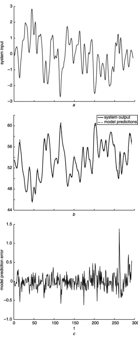
Fig. 3 Modelling results for example 3

a System input

b Model prediction and model output

c Model prediction error

[image:7.612.39.271.176.365.2] [image:7.612.301.533.180.753.2] [image:7.612.44.260.408.753.2]

small coefficient for D-optimality). The iterative procedure of the proposed algorithm was applied. The model was automatically terminated at 66 centres. The final basis pursuit parameter was derived at l¼1:7108: The modelling MSE for the test data set is derived at 1:36

105:Equivalently a 99:94%output variance of the test data has been explained by the model. To illustrate the overall performance of the model in capturing the underlying system dynamics the modelling results for both estimation and test data set 5 are shown inFig. 2.

4.3

Example 3

The benchmarking gas furnace data (series J in [23]) set consists of 296 input=output pairs representing coded input gas-feed rate as input,u(t), andCO2concentration from the

gas furnace as outputy(t). All the data were used as training data set. A RBF network with the input vector xðtÞ ¼ ½uðt1Þ;uðt2Þ;uðt3Þ;yðt1Þ;yðt2Þ;yðt3ÞT_{; and}

the thin-plate-spline basis function piðxðtÞÞ ¼ kxðtÞ cik2logkxðtÞ cikwas used as the basis function with all

data sets as candidate centresci:

The iterative procedure of the proposed algorithm was applied with b¼104: The model was automatically terminated at 36-centres. The final basis-pursuit parameter was derived atl¼0:0052:The modelling MSE for the test data set is derived at 0.045. A list of results on the same data can be found in[24]. It can be seen that the results obtained in this study are comparable. The modelling results for both estimation and test data sets are shown inFig. 3.

5 Conclusions

This paper has introduced a model identification algorithm for linear-in-the-parameters models. The pro-posed approach is based on the forward orthogonal least-square algorithm using the modified Gram – Schmidt procedure. The approach aims to simultaneously optimise the model approximation ability, sparsity and robustness by combining the modified Gram – Schmidt algorithm with basis pursuit and D-optimality design. The main contribution is to tune the model parameters, in each forward regression step, with the basis pursuit that minimises the l1 norm of the parameter estimates vector. The D-optimality design criterion is used for model selection to ensure the model robustness and automati-cally terminates at a sparse model. The choice of basis-pursuit parameters is discussed and a simple iterative procedure of the proposed algorithm is introduced to obtain a model with good generalisation. Both the parameter tuning procedure, based on basis pursuit, and the model selection criterion, based on the D-optimality that is effective in ensuring model robustness, are integrated with forward regression to maintain compu-tational efficiency.

6 Acknowledgments

XH gratefully acknowledges that part of this work was supported by the UK EPSRC. The authors would like to thank the referees for their constructive comments.

7 References

1 Harris, C.J., Hong, X., and Gan, Q.: ‘Adaptive modelling, estimation and fusion from data: a neurofuzzy approach’ (Springer-Verlag, Berlin, 2002)

2 Brown, M., and Harris, C.J.: ‘Neurofuzzy adaptive modelling and control’ (Prentice Hall, Hemel Hempstead, 1994)

3 Bossley, K.M.: ‘Neurofuzzy modelling approaches in system identifi-cation’. PhD thesis, Dept of ECS, University of Southampton, 1997 4 Murray-Smith, R., and Johansen, T.A.: ‘Multiple model approaches to

modelling and control’ (Taylor and Francis, London, 1997)

5 Bellman, R.: ‘Adaptive control processes’ (Princeton University Press, Princeton, 1966)

6 Jang, J.S.R., Sun, C.T., and Mizutani, E.: ‘Neurofuzzy and soft computing: a computational approach to learning and machine intelligence’ (Prentice Hall, Upper Saddle River, NJ, 1997)

7 Takagi, T., and Sugeno, M.: ‘Fuzzy identification of systems and its applications to modelling and control’,IEEE Trans. Syst. Man Cybern., 1985,15, pp. 116 – 132

8 Chen, S., Billings, S.A., and Luo, W.: ‘Orthogonal least squares methods and their applications to nonlinear system identification’,Int. J. Control, 1989,50, pp. 1873 – 1896

9 Chen, S., Wu, Y., and Luk, B.L.: ‘Combined genetic algorithm optimization and regularized orthogonal least-squares learning for radial basis function networks’,IEEE Trans. Neural Netw., 1999,10, pp. 1239 – 1243

10 Orr, M.J.L.: ‘Regularisation in the selection of radial basis function centers’,Neural Comput., 1995,7, (3), pp. 954 – 975

11 Akaike, H.: ‘A new look at the statistical model identification’,IEEE Trans. Autom. Control, 1974,19, pp. 716 – 723

12 Hansen, P.C.: ‘Rank-deficient and discrete ill-posed problems’ (SIAM, Philadelphia, 1998)

13 Neal, R.M., and Zhang, J.: ‘Classification for high dimensional problems using bayesian neural networks and dirichlet diffusion trees’. Presented at the NIPS Workshop on Feature Selection, Whistler, BC, 11 – 13 December 2003

14 Atkinson, A.C., and Donev, A.N.: ‘Optimum experimental designs’ (Clarendon Press, Oxford, 1992)

15 Hong, X., and Harris, C.J.: ‘Nonlinear model structure detection using optimum experimental design and orthogonal least squares’,IEEE Trans. Neural Netw., 2001,12, (2), pp. 435 – 439

16 Hong, X., and Harris, C.J.: ‘Nonlinear model structure design and construction using orthogonal least squares and D-optimality design’,

IEEE Trans Neural Netw., 2001,13, (5), pp. 1245 – 1250

17 Chen, S.: ‘Locally regularised orthogonal least squares algorithm for the construction of sparse kernel regression models’. Proc. 6th. Int. Conf. on Signal Processing, Beijing, China, 26 – 30 August 2002, pp. 1229 – 1232

18 Chen, S., Hong, X., and Harris, C.J.: ‘Sparse kernel regression modelling using combined locally regularised orthogonal least squares and D-optimality experimental design’,IEEE Trans. Autom. Control, 2003,48, (6), pp. 1029 – 1036

19 MacKay, D.J.C.: ‘Bayesian methods for adaptive models’. PhD thesis, California Institute of Technology, USA, 1991

20 Chen, S.S., Donoho, D.L., and Saunders, M.A.: ‘Atomic decomposition by basis pursuit’,SIAM Rev., 2001,43, (1), pp. 129 – 159

21 Efron, B., Hastie, T., Johnstone, I., and Tibshirani, R.: ‘Leastangle regression’,Ann. Sta., 2004,32, pp. 407 – 451

22 Ikeda, K.: ‘Multiple-valued stationary state and its instability of the transmitted light by a ring cavity system’,Opt. Commun., 1979,30, (2), pp. 257 – 261

23 Box, G.E.P., and Jenkins, G.M.: ‘Time series analysis, forecasting and control’ (Holden-Day, London, 1976)