Modelling Truncated and Clustered Count Data

M

T

C

C

D

A

S

,

R

C

A

Count response data often exhibit departures from the assumptions of standard Poisson

generalized linear models (McCullagh & Nelder 1989). In particular, cluster level correlation

of the data and truncation at zero are two common characteristics of such data. In this paper

we describe a random components truncated Poisson model that can be applied to clustered

and zero-truncated count data. Residual maximum likelihood method estimators for the

parameters of this model are developed and their use illustrated using a data set of non-zero

counts of sheets with edge strain defects in iron sheets produced by the Mobarekeh Steel

Complex, Iran. We also report on a small scale simulation study that supports the estimation

procedure.

Modelling Truncated and Clustered Count Data

Ayoub Saei and Ray Chambers

Southampton Statistical Sciences Research Institute, University of Southampton, Highfield, Southampton, SO17 1BJ, United Kingdom

Summary

Count response data often exhibit departures from the assumptions of standard Poisson generalized linear models (McCullagh & Nelder 1989). In particular, cluster level correlation of the data and truncation at zero are two common characteristics of such data. In this paper we describe a random components truncated Poisson model that can be applied to clustered and zero-truncated count data. Residual maximum likelihood method estimators for the parameters of this model are developed and their use illustrated using a data set of non-zero counts of sheets with edge strain defects in iron sheets produced by the Mobarekeh Steel Complex, Iran. We also report on a small scale simulation study that supports the estimation procedure.

Key words: Cluster, Poisson, Random components, REML, Truncated.

1. Introduction

defects observed. Unfortunately, no information was collected on sheets with no edge defects, nor was there a count of the number of such sheets. Consequently information on numbers of sheets with edge defects was only available for days on which there was at least one sheet with such defects.

A flexible and the most widely used model for analysing count response data is the Poisson generalized linear model (McCullagh & Nelder, 1989 Chap. 6). In our case however these data are truncated at zero. The distribution of strictly positive Poisson count data is called the zero-truncated Poisson and has a long history, dating back to the papers of David & Johnson (1952) and Plackett (1953). See also Johnson, Kotz & Kemp (1992). Shaw (1988) extends the Poisson generalized linear model (PGLM) of McCullagh & Nelder (1989) to deal with truncated count data. Alternatively, zero truncated count data can be modelled via the negative binomial generalized linear model (NBGLM), see Gurmu (1991) and Grogger & Carson (1991). Gurmu & Trivedi (1992) present tests for overdispersion in the truncated count model. The truncated Poisson generalized linear model (TPGLM) has been applied to adenomatous polyps data by Xie & Aicken (1997). Examples of economic applications of the TPGLM are given in Cameron & Trivedi (1998 Chap. 1).

In many applications, however, the dependence structure is more complex than the independent observations assumed by the TPGLM. In particular, count data often exhibit clustering, with observations within clusters correlated with one another. A typical example of this is where repeated measurements are taken of a single subject and a cluster consists of the set of observations for this subject. Ignoring such clustering effects in the TPGLM leads to overdipersion and can result in biased and inconsistent estimates of the regression coefficients in the model (Grogger & Carson, 1991).

Sections 2 and 3 define the random effects TPGLM and estimation procedures for model parameters respectively. Section 4 then sets out results from a small simulation study that explores the behaviour of these estimators, while Sections 5 contains a description of their application to the MSC data set on edge strain defects for iron sheets. The results of the paper are discussed in Section 6.

2. Model Specification

In what follows i = 1, 2, ..., N denotes a cluster and t = 1,2, ... , denotes an observation within a cluster. Let Y

ni

it represent the value that a count response variable Y takes at observation t within cluster i. In our application, i denotes day and t denotes time within day, we will refer to these indices as day and time from now on. We assume that , while the data collection process is such that only strictly positive values of Y

) Pn(

d

it it

Y = η

it are observed. We consider two different models for λit. In the first, ηit = ln(λit) is assumed to be a linear function of a vector xit of p covariates as well as a random day effect u1i to account for variation not explained by the values in xit. That is,

(1)

i it it u1

T +

=x β

η

where β is an unknown vector of regression coefficients. The random effects u1i are assumed to be realisations of independent N(0, φ1) random variables.

In the second model ηit includes an extra random effect u2i, allowing a possible change in variance and pattern of association in the second and following observations within a day. This is consistent with the idea that the any day departures from the model in the first time period (first observation in a day) are likely to be carried over into subsequent time periods(in subsequent observations in a day) and to be augmented further errors. This model is

(2)

i t i it

it u1 u2

T ∆

η = x β + +

where ∆t = I(t >1), ( , ) N( , ) and

d

2

1 = 0 Φ

= _{i i}

i u u

u

. (3) ⎥

⎦ ⎤ ⎢

⎣ ⎡ =

2 3

3 1

φ φ

φ φ

Φ

important to realise that a negative value for uˆ_2i implies a larger decline in ηit, so that small Y observations are likely (an improvement in the production lines).

Let ( , ,..., ),

1 1 12 11

1 = u u uN

u ( , ,..., )

2 2 22 21

2 = u u u N

u and let Z1, Z2 denote the

incidence matrices for the random effects vectors u1 and u2 respectively. Let N1 denote

the number of the clusters N2 the number of the clusters with more than one

observation. In general the model for η=(η_it, i=1,2,...,N, t=1,2,...,n_i) can be expressed as η= Xβ +Zu, where X is a known matrix of regression variables, Z = Z1

and u = u1 under (1) and Z = [Z1, Z2] and u=(u1,u2) under (2). The random vectors u1

and u are distributed as multivariate normal with zero mean vectors and variance-covariance matrices given by

1 1IN

A=φ and _⎥ respectively,

⎦ ⎤ ⎢

⎣ ⎡ =

2 1

2 T 3

3 1

N N

J

J

I I

A φ_{φ φ}φ

where J is given by deleting the columns of the identity matrix that correspond to clusters with a single observation.

1

N

I

3. Model Estimation

Henderson (1963, 1973a, and 1975) develops best linear unbiased predictors for linear mixed models. These ideas have been extended to obtain maximum likelihood (ML) and restricted or residual maximum likelihood (REML) estimators in Harville (1977), Thompson (1980), Fellner (1986, 1987) and Speed (1991). McGilchrist (1994) extends this approach to generalized linear mixed models. This method has elements in common with Schall (1991), Breslow & Clayton (1993), Wolfinger (1993), Nelder & Lee (1996) and Saei & McGilchrist (1998). Lee & Nelder (2001a, 2001b) further extend the work of Nelder & Lee (1996) to correlated non-normal data. Below we outline the extension of this approach to the random component truncated Poisson model.

Let l1 be the loglikelihood function of truncated Poison observations conditional

on the value of the random component vector u and let l2 be the logarithm of the

probability density function of u. For the model (2) the functions l1 and l2 are

∑ ∑

= N i

n

t it it it it it

i

y y

l

1 1

) | | ln . ( 2

1 T 1

2 A u A u

− + + − = const l

respectively. Penalised likelihood (PL) estimates and are obtained by maximising l = l

β~ u~

1 + l2 with respect to β and u respectively. These estimates are then used as an

initial step in finding ML and REML estimates of φj via Anderson (1973) and Henderson (1973b) algorithm. The iterative procedure used to obtain the ML and REML estimators and their approximate variance-covariance matrices can be specified as follows:

(a) Starting from initial values β₀, u0 and φj0 (hence A0) successive iterations are

obtained by finding changes ∆β and ∆uto the current estimates from the equations ⎥ ⎦ ⎤ ⎢ ⎣ ⎡ − ∂ ∂ = ⎥ ⎦ ⎤ ⎢ ⎣ ⎡ − 0 1 0 0 1 T u A 0 W u V η β l ∆ ∆ (4)

where W = [X, Z], η₀ =Xβ₀+Zu₀ and _⎥ ⎦ ⎤ ⎢ ⎣ ⎡ + ∂ ∂ ∂ −

= ₋₁

0 T 0 0 1 2 T ) ( A 0 0 0 W W V η η l ; T 0 0 1 2 0

1/∂η and ∂ /∂η ∂η

∂l l are first and second order derivatives of l1 with

respect to η andevaluated at initial value η0.

(b) Once iterations of (4) have converged to β~ and u~, let η~=Xβ~+Z~u,

T 1

2 ~ ~

/∂η∂η

∂ l − =

B , T* =[T_jk*]=[A₀−1+ZTBZ]−1, a1 = 1 1 T 1 * 11 1 ~ ~ )

tr(BT +u Bu , a2 = 2 T 2 * 22 ~ ~ )

tr(T +u u , a3 = 2 1 T 1 * 11 2 ~ ~ )

tr(BT +u B u and 2(tr( ) ~T ~₂)

1 T * 12

4 T J u Ju

a = + . B1 is a

diagonal matrix with entry if the corresponding cluster has a single observation and 1 otherwise, while B

2 20 10 2 2 30 20

10 ) /( )

(φ φ −φ φ φ

2 is a diagonal matrix with

diagonal element zero if the corresponding cluster has a single observation and 1 otherwise. The estimates of φj are then given by

(c) The preceding two steps are then repeated, with initial values set to β~, u~ and .

j

φˆ

At convergence, φˆ_j is the ML estimate φˆ_j(ML) of φj. The asymptotic variance-covariance matrix for φˆ_(ML)=(φˆ_1(ML), φˆ_2(ML) ,φˆ_3(ML)) is

(6) 1 333 233 133 323 223 123 322 222 122 313 213 113 312 212 112 311 211 111 (ML) 2 2 2 2 2 2 2 ) ˆ var( − ⎥ ⎥ ⎥ ⎦ ⎤ ⎢ ⎢ ⎢ ⎣ ⎡ − + − + − + − + − + − + = r r r r r r r r r r r r r r r r r r φ where )) ( ) ( ( tr 1 1 1 k j jk r φ φ ∂ ∂ ∂ ∂

= A A− A A−

)) ( ) ( ( tr 1 * 1 * 2 k j jk r φ φ ∂ ∂ ∂ ∂

= T A− T A−

)) ( ) ( ( tr 1 * 1 3 k j jk r φ φ ∂ ∂ ∂ ∂

= A A− T A−

for j, k = 1, 2, 3.

Let _⎥ and

⎦ ⎤ ⎢ ⎣ ⎡ = 22 21 12 11 V V V V V _⎥ ⎦ ⎤ ⎢ ⎣ ⎡ = − 22 21 12 11 1 T T T T

V denote the partitions of the matrix V and its

inverse corresponding to the dimensions of β and u. Replacing T* by T22 in (5) and

(6) yields the REML estimate φˆj(REML) of φj and the variance-covariance matrix for the REML estimators φˆ_(REML) =(φˆ_1(REML),φˆ_2(REML),φˆ_3(REML)) respectively.

4. Simulations

A limited simulation study was undertaken to examine the performance of the method. Truncated count observations were generated from the one random component truncated Poisson model, ηit= β0 + xitβ1 + u1i and the two random component truncated Poisson model, ηit = β0 + xitβ1 + u1i + ∆tu2i. The values of u1i were independently generated from normal distribution with zero mean and variance φ1 in the first model.

were randomly assigned to values of zero or one. Observations were generated for times t = 1, 2, …, 5 and for subjects i = 1, 2, …, 30. The TPGLM was then fitted to these data

and estimates of φ1, φ2, φ3, β0, and β1 obtained, as well as the mean deviance (MD) and

lower and upper confidence intervals for β0 and β1 (with α = 0.05). This process was

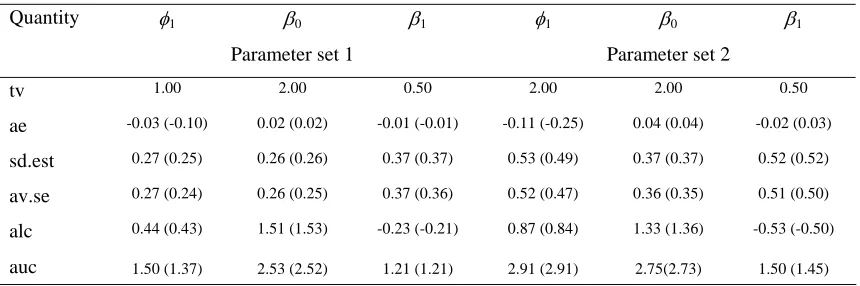
then independently replicated 10000 times. Table 1 defines the quantities reported in simulation results set out in tables 2 – 6. Tables 3 – 6 show the results by both ML (in brackets) and REML methods.

Table 1 about here

Table 2 shows the results from fitting the TPGLM via ML to truncated observations generated by one and two random components TPGLMs. Corresponding results from REML and ML (in brackets) fits of a one random component TPGLM are set out in Table 3.

Tables 2 and 3 about here

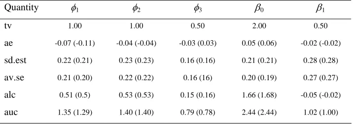
Tables 4 and 5 explores the impact of model misspecification, showing the results from REML and ML fits of a one and a two random components TPGLM to data generated by a two correlated random components model. In comparison, Table 6 shows what happens when the correct two component model is fitted to the two component data.

Tables 4 – 6 about here

The results set out in Table 2 show that the ML estimators of β0 and β1 under the

standard TPGLM are seriously biased when applied to observations generated under random components TPGLM. This bias increases from one component random effect to the two correlated random components. It is also increases with the size of the variance component in the random components TPGLM. The average mean deviances (amd) are very far from 1 in all cases and the average 95% confidence limits (alc, auc) exclude the true values of the parameters β0 and β1. The average estimated standard errors (av.se)

are also much smaller than their corresponding simulation standard errors (sd.est) of the estimates of these parameters.

of the regression parameters. The simulation standard errors sd.est of the parameter estimators agrees with their average estimated standard errors av.se under both ML and REML. This is also true for the φ1, φ2 and φ3. Although not shown here, increasing the

number of observations for each subject from 5 to 15 significantly decreased the biases of the parameter estimators and their estimated variances. We also see that in all cases the average 95% confidence limits (alc, auc) contain the true values of β0, β1, φ1,φ2 and

φ3.

Finally, in Tables 4 and 5 we show that the effect of model misspecification when fitting a random components TPGLM. In these cases we fitted a one random component TPGLM and a two independent random components to data generated from a two correlated random components TPGLM. This led to positively biased variance component estimators and increased bias for the estimators of β0 and β1 for the one

random component model. These biases are small when we ignore the covariance between the two random components. The “average” confidence interval does not include the true value for φ1 in Table 4.

5. Application to Iron Sheet Data

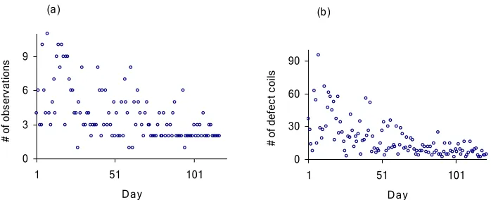
series structure for the random effects would have been appropriate. However, in the absence of any information in this regard, we decided to persist with the simple two component random effects model for these data. Figure 1(b) shows number of coils with edge strain defect.

(a)

0 3 6 9

1 51 101

Day

# of

obs

er

va

tions

(b)

0 30 60 90

1 51 101

Day

# of

def

ec

t c

oi

ls

Figure 1. (a) Number of observations on each 122 days; (b) number of coils with edge strain defect over 122 days.

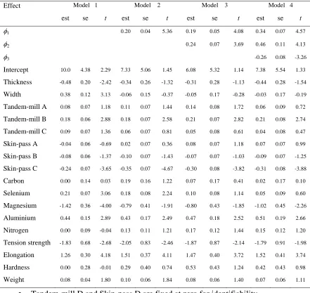
Table 7 sets out the parameter estimates and associated standard errors for four zero-truncated Poisson GLMs fitted to these data, with the response variable in each case corresponding to the number of sheets with edge strain defects observed on each day. Model 1 is the standard TPGLM, fitted via ML. Model 2 is a one random effect TPGLM, fitted via REML, with the random effect corresponding to day of observation. Model 3 is a two independent random effects TPGLM, with an extra random effect introduced to allow for within day heterogeneity. Finally, Model 4 relaxes the independent assumption in model 3 and includes an extra parameter to account for dependence between two random effects. Models 3 and 4 are also fitted using REML.

Examination of the results for Model 4 in Table 7 show that there is statistically significant variation between days ( = 0.34 with an estimated standard error of 0.07). This day effect varies significantly within a day ( = 0.46 with an estimated standard error of 0.11). Furthermore the two random effects are correlated with estimated covariance of = -0.26 and estimated standard error of 0.08. The estimated correlation between two random effects is

1

ˆ φ

2

ˆ φ

3

ˆ φ

identified for further study. Under Models 2, 3 and 4, neither sheet thickness nor sheet width effects are statistically significant. In contrast, under Model 1 (TPGLM) both sheet width and sheet thickness are highly significant. There are also significant tandem-mill and skin-pass process effects, with Wald statistics ( ) of 9.96 and 23.2 respectively. However, with the exception of magnesium and selenium, the conclusions are the same for the remaining covariates under all four models. The selenium does not have significant effect under both models 3 and 4 whereas magnesium does have a significant effect under only model 4. In contrast, under both Model 1 (TPGLM) and Model 2 (single random component TPGLM) selenium and magnesium (marginally for model 2) are significant. The aluminium, elongation and tension strength are other significant covariates. This conclusion is supported by all four models.

β β βˆT_[var( ˆ_)]−1 ˆ

Table 7 about here

6. Summary and Discussion

In this paper we introduce a simple method for analysing longitudinal or repeated measurement count response data that are truncated at zero. Two types of models, one involving a single random component to account for between subject heterogeneity, and a second involving two random components, with the second component used to account for within subject heterogeneity, have been investigated. These random components are allowed to be correlated. When applied to zero truncated data on counts of coils with edge defects in iron sheets produced at the Mobarekeh Steel Complex, the two random components model indicates the existence of statistically significant day to day and within day heterogeneity in these data. The two random components are also significantly correlated. Furthermore, misleading inferences are obtained if the within day heterogeneity and the dependence between random components are ignored in model specification.

to be negatively biased. Increasing number of observation per cluster and clusters decreases the bias and improves the asymptotic performance of the REML estimators. Our inference is based on the asymptotic properties of the REML estimators. In general, the development of asymptotic properties is difficult for models with random effects. This difficulty is not specific to generalized linear mixed models (the approach taken in this paper). Jiang (1996) has investigated the asymptotic behaviour of REML estimators for linear mixed models. Breslow and Clayton (1993) have showed that for Poisson data the accuracy of these estimators improves as the mean increases. Lin (1997) has pointed out that REML estimator of variance components are not normally distributed unless the number of clusters is large and the estimators bounded away from zero. Using a Laplace approximation, Lin & Breslow (1996) show that the REML estimators are biased for large variance components and introduced a bias correction to improve the asymptotic performance of the REML estimators.

Turning now to ML estimation, we note that in theory ML estimates can be calculated via numerical integration using Gauss-Hermite quadrature. However, this is an impractical method for the models with high dimension random effects. More recently McCulloch (1997) and Booth & Hobert (1999) have explored the use of Markov Chain Monte Carlo (MCMC) and Monte Carlo EM in this context. These are computer intensitive approaches and their application to the complex models is very difficult (if not impossible). They also require fairly sophisticated computer programming since there is no generally available software.

Finally, we note that the translated Poisson distribution, defined by Pr(Yit = yit) = exp(-λit) /( y

1

−

it

y it

λ it - 1)! is an alternative to the truncated Poisson distribution for positive response values. The application of this model via the specification ln(µit - 1) =

, i.e., a fixed effect model, to the iron sheet data yielded a mean deviance of 3.1 whereas the TPGLM without day random effect (TPGLM fixed effect model) had a mean deviance of 2.994. Clearly, further research needs to be done to explore alternative models for positive valued data.

β

T

it it =x

Acknowledgments

The first author’s research was partially supported by research council of Isfahan University of Technology. The authors thank the associate Editor and a referee for their helpful comments.

References

Anderson, T.W. (1973). Asymptotically efficient estimation of covariance matrices with linear structure. Ann. Statist. 1, 135 - 141.

Booth, J.G. & Hobert, J.P. (1999). Maximizing generalized linear mixed model likelihoods with an automated Monte Carlo EM algorithm. J. Roy. Statist. Soc. Ser. B 61, 265 - 285.

Breslow, N.E. & Clayton, D.G. (1993). Approximate inference in generalised linear mixed models. J. Amer. Statist. Assoc. 88, 9 - 25.

Cameron, A.C. & Trivedi, P. (1998). Regression analysis of count data. Cambridge University Press, Cambridge.

David, F.N. & Johnson, N.L. (1952). The truncated Poisson. Biometrics 8, 275 - 285. Gurmu, S. (1991) Tests for detecting overdispersion in the positive Poisson regression

model. J. Bus. Econom. Statist. 9, 215 - 222.

Gurmu, S. & Trivedi (1992). Overdispersion tests for truncated Poisson regression models. J. Econometrics 54, 347 - 370.

Grogger, J.T. & Carson, R.T. (1991). Models for truncated counts. J. Appl. Econometrics 6, 225 - 238.

Henderson, C.R. (1963). Selection index and expected genetic advance. In Statistical Genetics and Plant Breeding (W.D. Hanson and H.F. Robinson, eds.), 141 - 163.

National Academy of Sciences and National Research Council Publication No. 982, Washington, D.C.

Henderson, C.R. (1973a). Sire evaluation and genetic trends. In Proceedings of the Animal Breeding and Genetics Symposium in Honour of Dr. Jay L. Lush 10-41.

Amer. Soc. Animal Sci.-Amer. Dairy Sci. Assn.-Poultry Sci. Assn. Champaigne, Illinois.

Henderson, C.R. (1975). Best linear unbiased estimation and prediction under selection model. Biometrics 31, 423 - 447.

Jiang, J. (1996). REML estimation: asymptotic behaviour and related topic. Ann. Statist. 24, 255 - 286.

Johnson, N.L., Kotz, S. & Kemp, A.W. (1992). Univariate discrete distributions. Second Ed. John Wiley & Sons, Inc.

Lee, Y. & Nelder, J.A. (2001a). Hierarchical generalized linear models: A synthesis of generalised linear models, random-effect model and structured dispersions. Biometrika 88, 987 - 1006.

Lee, Y. & Nelder, J.A. (2001b). Modelling and analysing correlated non-normal data. Statistical Modelling 1, 3 - 16

Lin, X. & Breslow, N.E. (1996). Bias correction in generalized linear mixed model with multiple components of dispersion. J. Amer. Statist. Assoc. 91, 1007 - 1016. McCullagh, P. (1980). Regression models for ordinal data. J. Roy. Statist. Soc. Ser. B,

42, 109 - 142.

McCullagh, P. & Nelder, J.A. (1989). Generalized linear models. Second Ed. London: Chapman and Hall.

McCulloch, C.E. (1997). Maximum likelihood algorithms for generalized linear mixed models. J. Amer. Statist. Assoc. 92, 162 - 170.

McGilchrist, C.A. (1994). Estimation in generalized mixed models. J. Roy. Statist. Soc. Ser. B 56, 61 - 69.

Nelder, J.A. & Lee, Y. (1996). Hierarchical generalized linear models. J. Roy. Statist. Soc. Ser. B 58, 619-678.

Plackett, R.L. (1953). The truncated Poisson distributions. Biometrics 9, 485 - 488. Saei, A. & McGilchrist, C. (1998). Longitudinal threshold models with random

components. The Statistician (JRSS Series D) 47, 365 - 375.

Schall, R (1991). Estimation in generalised linear models with random effects. Biometrika 78, 719 - 727.

Shaw, D. (1988). One-site samples’ regression problems of non-negative integers, truncation, and endogenous stratification. J. Econometrics 37, 211 - 223.

Wolfinger, R. (1993). Laplace’s approximation for nonlinear mixed models. Biometrika 80, 791 - 796.

Table 1 Definitions of quantities reported in simulation results set out in tables 2 – 6. Quantity Description

tv true parameter values ae average error

sd.est actual standard error over 10000 simulations av.se average estimated standard error

alc average lower 95% confidence limit auc average upper 95% confidence limit amd average mean deviance

Table 2 Simulation results for the ML fit of the TPGLM to data generated from one and two random component truncated Poisson models; see Table 1 for definitions.

1 Component Model 2 Components Model

Quantity φ1 β0 β1 φ1 φ2 φ3 β0 β1 φ1 φ2 φ3 β0 β1

Parameter set 1 Parameter set 2

tv 1.00 2.00 0.50 1.00 1.00 0.00 2.00 0.50 1.00 1.00 0.50 2.00 0.50

ae 0.45 -0.03 0.65 -0.13 0.74 -0.19

sd.est 0.30 0.41 0.35 0.46 0.37 0.51

av.se 0.03 0.05 0.03 0.04 0.03 0.04

alc 2.37 0.38 2.59 0.28 2.67 0.23

auc 2.51 0.56 2.71 0.45 2.80 0.39

amd 13.45 20.80 24.50

Table 3 Simulation results for the REML (ML) fit to data generated from a one random component truncated Poisson model; see Table 1 for definitions.

Quantity φ1 β0 β1 φ1 β0 β1

Parameter set 1 Parameter set 2

tv 1.00 2.00 0.50 2.00 2.00 0.50

ae -0.03 (-0.10) 0.02 (0.02) -0.01 (-0.01) -0.11 (-0.25) 0.04 (0.04) -0.02 (0.03)

sd.est 0.27 (0.25) 0.26 (0.26) 0.37 (0.37) 0.53 (0.49) 0.37 (0.37) 0.52 (0.52)

av.se 0.27 (0.24) 0.26 (0.25) 0.37 (0.36) 0.52 (0.47) 0.36 (0.35) 0.51 (0.50)

alc 0.44 (0.43) 1.51 (1.53) -0.23 (-0.21) 0.87 (0.84) 1.33 (1.36) -0.53 (-0.50)

Table 4 Simulation results for REML (ML) fit of a one random component truncated Poisson model to data generated from a two correlated random components truncated

Poisson model; see Table 1 for definitions.

Quantity φ1 φ2 φ3 β0 β1

tv 1.00 1.00 0.50 2.00 0.50

ae 0.97 (1.03) 0.10 (0.11) -0.02 (-0.02)

sd.est 0.57 (0.55) 0.40 (0.39) 0.56 (0.56)

av.se 0.58 (0.54) 0.39 (0.38) 0.55 (0.53)

alc 0.83 (0.98) 1.34 (1.37) -0.60 (-0.56)

auc 3.11 (3.10) 2.87 (2.84) 1.57 (1.52)

Table 5 Simulation results for REML (ML) fit of a two independent random components truncated Poisson model to data generated from a two correlated random

components truncated Poisson model; see Table 1 for definitions. Quantit

y φ1 φ2 φ3 β0 β1

tv 1.00 1.00 0.50 2.00 0.50

ae 0.03 (-0.05) -0.04 (-0.04) 0.02 (0.03) -0.02 (-0.02)

sd.est 0.32 (0.29) 0.29 (0.29) 0.29 (0.29) 0.40 (0.40)

av.se 0.31 (0.28) 0.29 (0.29) 0.28 (0.27) 0.40 (0.38)

alc 0.43 (0.41) 0.38 (0.39) 1.46 (1.49) -0.30 (-0.27)

auc 1.64 (1.49) 1.53 (1.53) 2.57 (2.56) 1.26 (1.23)

Table 6 Simulation results for REML (ML) fit to data generated from a two correlated random components truncated Poisson model; see Table 1 for definitions.

Quantity φ1 φ2 φ3 β0 β1

tv 1.00 1.00 0.50 2.00 0.50

ae -0.07 (-0.11) -0.04 (-0.04) -0.03 (0.03) 0.05 (0.06) -0.02 (-0.02)

sd.est 0.22 (0.21) 0.23 (0.23) 0.16 (0.16) 0.21 (0.21) 0.28 (0.28)

av.se 0.21 (0.20) 0.22 (0.22) 0.16 (16) 0.20 (0.19) 0.27 (0.27)

alc 0.51 (0.5) 0.53 (0.53) 0.15 (0.16) 1.66 (1.68) -0.05 (-0.02)

Table 7 Parameter estimates (est), standard errors (se) and t (t = est/se) for four models fitted to the MSC iron sheet data.

Effect Model 1 Model 2 Model 3 Model 4 est se t est se t est se t est se t

φ1 0.20 0.04 5.36 0.19 0.05 4.08 0.34 0.07 4.57

φ2 0.24 0.07 3.69 0.46 0.11 4.13

φ3 -0.26 0.08 -3.26

Intercept 10.0 4.38 2.29 7.33 5.06 1.45 6.08 5.32 1.14 7.38 5.54 1.33

Thickness -0.48 0.20 -2.42 -0.34 0.26 -1.32 -0.31 0.28 -1.13 -0.44 0.28 -1.54

Width 0.38 0.12 3.13 -0.06 0.15 -0.37 -0.05 0.17 -0.28 -0.03 0.17 -0.19

Tandem-mill A 0.08 0.07 1.18 0.11 0.07 1.44 0.14 0.08 1.72 0.06 0.09 0.72

Tandem-mill B 0.18 0.06 2.88 0.18 0.07 2.58 0.21 0.07 2.82 0.21 0.08 2.74

Tandem-mill C 0.09 0.07 1.36 0.06 0.07 0.81 0.05 0.08 0.61 0.04 0.08 0.47

Skin-pass A -0.04 0.06 -0.69 0.02 0.07 0.36 0.08 0.07 1.18 0.07 0.07 0.99

Skin-pass B -0.08 0.06 -1.37 -0.10 0.07 -1.43 -0.07 0.07 -1.03 -0.09 0.07 -1.25

Skin-pass C -0.24 0.07 -3.65 -0.35 0.07 -4.67 -0.30 0.08 -3.82 -0.31 0.08 -3.88

Carbon 0.00 0.14 0.03 0.19 0.16 1.22 0.07 0.17 0.41 0.02 0.17 0.10

Selenium 0.21 0.07 3.06 0.18 0.08 2.24 0.10 0.08 1.14 0.05 0.09 0.60

Magnesium -1.42 0.36 -4.00 -0.79 0.41 -1.91 -0.80 0.43 -1.85 -1.02 0.45 -2.26

Aluminium 0.44 0.15 2.89 0.43 0.17 2.49 0.47 0.18 2.52 0.51 0.19 2.66

Nitrogen 0.00 0.09 -0.04 0.13 0.11 1.21 0.17 0.12 1.44 0.15 0.12 1.20

Tension strength -1.83 0.68 -2.68 -2.05 0.83 -2.46 -1.87 0.87 -2.14 -1.79 0.91 -1.98

Elongation 1.26 0.30 4.18 1.51 0.37 4.11 1.47 0.40 3.72 1.52 0.41 3.74

Hardness 0.00 0.28 -0.01 0.29 0.40 0.74 0.53 0.43 1.24 0.42 0.43 0.98

Weight 0.08 0.04 1.80 0.10 0.06 1.84 0.08 0.06 1.40 0.07 0.06 1.11 • Tandem-mill D and Skin-pass D are fixed at zero for identifiability

• Model 1 = TPGLM

• Model 2 = A one random component truncated Poisson model

• Model 3 = A two independent random components truncated Poisson model