Computational
Intelligence
An Introduction
Andries P. Engelbrecht
University of Pretoria
South Africa
Copyright © 2002 John Wiley & Sons Ltd, The Atrium, Southern Gate, Chichester, West Sussex P019 8SQ, England
Telephone (+44) 1243 779777
Email (for orders and customer service enquiries): [email protected] Visit our Home Page on www.wileyeurope.com or www.wiley.com
All Rights Reserved. No part of this publication may be reproduced, stored in a retrieval system or transmitted in any form or by any means, electronic, mechanical, photocopying, recording, scanning or otherwise, except under the terms of the Copyright, Designs and Patents Act 1988 or under the terms of a licence issued by the Copyright Licensing Agency Ltd, 90 Tottenham Court Road, London W1T 4LP, UK, without the permission in writing of the Publisher. Requests to the Publisher should be addressed to the Permissions Department, John Wiley & Sons Ltd, The Atrium, Southern Gate, Chichester, West Sussex PO19 8SQ, England, or emailed to [email protected], or faxed to (+44) 1243 770571.
This publication is designed to provide accurate and authoritative information in regard to the subject matter covered. It is sold on the understanding that the Publisher is not engaged in rendering professional services. If professional advice or other expert assistance is required, the services of a competent professional should be sought.
Other Wiley Editorial Offices
John Wiley & Sons Inc., 111 River Street, Hoboken, NJ 07030, USA Jossey-Bass, 989 Market Street, San Francisco, CA 94103-1741, USA Wiley-VCH Verlag GmbH, Boschstr. 12, D-69469 Weinheim, Germany
John Wiley & Sons Australia Ltd, 33 Park Road, Milton, Queensland 4064, Australia John Wiley & Sons (Asia) Pte Ltd, 2 Clementi Loop #02-01, Jin Xing Distripark, Singapore
129809
John Wiley & Sons Canada Ltd, 22 Worcester Road, Etobicoke, Ontario, Canada M9W 1L1
British Library Cataloguing in Publication Data
A catalogue record for this book is available from the British Library ISBN 0-470-84870-7
Typeset by the author.
Printed and bound in Great Britain by Biddies Ltd, Guildford and King's Lynn
To my parents, Jan and Magriet Engelbrecht, without whose loving support
Contents
List of Figures
XVII
Preface xx
Part I INTRODUCTION 1
1 Introduction to Computational Intelligence 3
1.1 Computational Intelligence Paradigms 5
1.1.1 Artificial Neural Networks 6
1.1.2 Evolutionary Computing 8
1.1.3 Swarm Intelligence 10
1.1.4 Fuzzy Systems 11
1.2 Short History 11
1.3 Assignments 13
Part II ARTIFICIAL NEURAL NETWORKS 15
2 The Artificial Neuron 17
2.1 Calculating the Net Input Signal 18
2.2 Activation Functions 18
2.3 Artificial Neuron Geometry 20
2.4 Artificial Neuron Learning 21
2.4.1 Augmented Vectors 22
2.4.2 Gradient Descent Learning Rule 22
2.4.3 Widrow-Hoff Learning Rule 24
2.4.4 Generalized Delta Learning Rule 24
2.4.5 Error-Correction Learning Rule 24
2.5 Conclusion 24
2.6 Assignments 25
3 Supervised Learning Neural Networks 27
3.1 Neural Network Types 27
3.1.1 Feedforward Neural Networks 28
3.1.2 Functional Link Neural Networks 29
3.1.3 Product Unit Neural Networks 30
3.1.4 Simple Recurrent Neural Networks 32
3.1.5 Time-Delay Neural Networks 34
3.2 Supervised Learning Rules 36
3.2.1 The Learning Problem 36
3.2.2 Gradient Descent Optimization 37
3.2.3 Scaled Conjugate Gradient 45
3.2.4 LeapFrog Optimization 47
3.2.5 Particle Swarm Optimization 48
3.3 Functioning of Hidden Units 49
3.4 Ensemble Neural Networks 50
3.5 Conclusion 52
3.6 Assignments 53
4 Unsupervised Learning Neural Networks 55
4.1 Background 55
4.2 Hebbian Learning Rule 56
4.3 Principal Component Learning Rule 58
4.4 Learning Vector Quantizer-I 60
4.5 Self-Organizing Feature Maps 63
4.5.1 Stochastic Training Rule 63
4.5.2 Batch Map 66
4.5.3 Growing SOM 67
4.5.4 Improving Convergence Speed 68
4.5.5 Clustering and Visualization 70
4.5.6 Using SOM 71
4.6 Conclusion 71
4.7 Assignments 72
5 Radial Basis Function Networks 75
5.1 Learning Vector Quantizer-II 75
5.2 Radial Basis Function Neural Networks 76
5.3 Conclusion 78
5.4 Assignments 78
6 Reinforcement Learning 79
6.1 Learning through Awards 79
6.2 Reinforcement Learning Rule 80
6.3 Conclusion 80
6.4 Assignments 81
7 Performance Issues (Supervised Learning) 83
7.1.1 Accuracy 84
7.1.2 Complexity 88
7.1.3 Convergence 89
7.2 Analysis of Performance 89
7.3 Performance Factors 90
7.3.1 Data Preparation 90
7.3.2 Weight Initialization 97
7.3.3 Learning Rate and Momentum 98
7.3.4 Optimization Method 101
7.3.5 Architecture Selection 101
7.3.6 Adaptive Activation Functions 108
7.3.7 Active Learning 110
7.4 Conclusion 118
7.5 Assignments 119
Part III EVOLUTIONARY COMPUTING 121
8 Introduction to Evolutionary Computing 123
8.1 Representation of Solutions - The Chromosome 124
8.2 Fitness Function 125
8.3 Initial Population 126
8.4 Selection Operators 126
8.4.1 Random Selection 127
8.4.2 Proportional Selection 127
8.4.3 Tournament Selection 128
8.4.4 Rank-Based Selection 129
8.5 Reproduction Operators 130
8.6 General Evolutionary Algorithm 130
8.7 Evolutionary Computing vs Classical Optimization 131
8.8 Conclusion 131
8.9 Assignments 132
9 Genetic Algorithms 133
9.1 Random Search 133
9.2 General Genetic Algorithm 134
9.3 Chromosome Representation 135
9.4 Cross-over 137
9.5 Mutation 138
9.6 Island Genetic Algorithms 141
9.7 Routing Optimization Application 142
9.8 Conclusion 144
9.9 Assignments 144
10 Genetic Programming 147
10.1 Chromosome Representation 147
10.2 Initial Population 149
10.3 Fitness Function 149
10.4 Cross-over Operators 151
10.5 Mutation Operators 151
10.6 Building-Block Approach to Genetic Programming 152
10.7 Assignments 154
11 Evolutionary Programming 155
11.1 General Evolutionary Programming Algorithm 155
11.2 Mutation and Selection 156
11.3 Evolutionary Programming Examples 156
11.3.1 Finite-State Machines 156
11.3.2 Function Optimization 158
11.4 Assignments 160
12 Evolutionary Strategies 161
12.1 Evolutionary Strategy Algorithm 161
12.2 Chromosome Representation 162
12.3 Crossover Operators 163
12.4 Mutation operators 164
12.5 Selection Operators 166
12.6 Conclusion 166
13 Differential Evolution 167
13.1 Reproduction 167
13.2 General Differential Evolution Algorithm 168
13.3 Conclusion 169
13.4 Assignments 169
14 Cultural Evolution 171
14.1 Belief Space 172
14.2 General Cultural Algorithms 173
14.3 Cultural Algorithm Application 174
14.4 Conclusion 175
14.5 Assignments 175
15 Coevolution 177
15.1 Coevolutionary Algorithm 178
15.2 Competitive Fitness 179
15.2.1 Relative Fitness Evaluation 179
15.2.2 Fitness Sampling 180
15.2.3 Hall of Fame 180
15.3 Cooperative Coevolutionary Genetic Algorithm 180
15.4 Conclusion 181
15.5 Assignments 182
Part IV SWARM INTELLIGENCE 183
16 Particle Swarm Optimization 185
16.1 Social Network Structure: The Neighborhood Principle 186
16.2 Particle Swarm Optimization Algorithm 187
16.2.1 Individual Best 187
16.2.2 Global Best 188
16.2.3 Local Best 189
16.2.4 Fitness Calculation 189
16.2.5 Convergence 189
16.3 PSO System Parameters 189
16.4 Modifications to PSO 191
16.4.1 Binary PSO 191
16.4.2 Using Selection 191
16.4.3 Breeding PSO 192
16.4.4 Neighborhood Topologies 193
16.5 Cooperative PSO 193
16.6 Particle Swarm Optimization versus Evolutionary Computing and Cultural Evolution 194
16.7 Applications 194
16.8 Conclusion 195
16.9 Assignments 195
17 Ant Colony Optimization 199
17.1 The "Invisible Manager" (Stigmergy) 199
17.2 The Pheromone 200
17.3 Ant Colonies and Optimization 201
17.4 Ant Colonies and Clustering 203
17.5 Applications of Ant Colony Optimization 206
17.6 Conclusion 208
17.7 Assignments 208
Part V FUZZY SYSTEMS 209
18 Fuzzy Systems 211
18.1 Fuzzy Sets 212
18.2 Membership Functions 212
18.3 Fuzzy Operators 214
18.4 Fuzzy Set Characteristics 218
18.5 Linguistics Variables and Hedges 219
18.6 Fuzziness and Probability 221
18.7 Conclusion 221
18.8 Assignments 222
19 Fuzzy Inferencing Systems 225
19.1 Fuzzification 227
19.2 Inferencing 227
19.3 Defuzzification 228
19.4 Conclusion 229
19.5 Assignments 229
20 Fuzzy Controllers 233
20.1 Components of Fuzzy Controllers 233
20.2 Fuzzy Controller Types 234
20.2.1 Table-Based Controller 236
20.2.2 Mamdani Fuzzy Controller 236
20.2.3 Takagi-Sugeno Controller 237
20.3 Conclusion 237
20.4 Assignments 238
21 Rough Sets 239
21.1 Concept of Discernibility 240
21.2 Vagueness in Rough Sets 241
21.3 Uncertainty in Rough Sets 242
21.4 Conclusion 242
21.5 Assignments 243
22 CONCLUSION 245
Bibliography 247
Further Reading 269
A Acronyms 271
B Symbols 273
B.I Part II - Artificial Neural Networks 273
B.11 Chapters 2-3 273
B.1.2 Chapter 4 274
B.1.3 Chapter 5 275
B.1.4 Chapter 6 275
B.1.5 Chapter 7 276
B.2 Part III - Evolutionary Computing 276
B.3 Part IV - Swarm Intelligence 277
B.3.1 Chapter 17 277
B.3.2 Chapter 18 277
B.4 Part V - Fuzzy Systems 278
B.4.1 Chapters 19-21 278
B.4.2 Chapter 22 278
Index 281
List of Figures
1.1 Illustration of CI paradigms 5
1.2 Illustration of a biological neuron 7
1.3 Illustration of an artificial neuron 8
1.4 Illustration of an artificial neural network 9
2.1 An artificial neuron 17
2.2 Activation functions 19
2.3 Artificial neuron boundary illustration 21
2.4 GD illustrated 23
3.1 Feedforward neural network 28
3.2 Functional link neural network 30
3.3 Elman simple recurrent neural network 33
3.4 Jordan simple recurrent neural network 34
3.5 A single time-delay neuron 35
3.6 Illustration of PU search space for f(z) = z3 44
3.7 Feedforward neural network classification boundary illustration ... 50
3.8 Hidden unit functioning for function approximation 51
3.9 Ensemble neural network 52
4.1 Unsupervised neural network 57
4.2 Learning vector quantizer to illustrate clustering 61
4.4 Visualization of SOM clusters for iris classification 73
5.1 Radial basis function neural network 77
6.1 Reinforcement learning problem 80
7.1 Illustration of overfitting 86
7.2 Effect of outliers 92
7.3 SSE objective function 93
7.4 Huber objective function 94
7.5 Effect of learning rate 99
7.6 Adaptive sigmoid 109
7.7 Passive vs active learning 113
9.1 Hamming distance for binary and Gray coding 135
9.2 Cross-over operators 139
9.3 Mutation operators 140
9.4 An island GA system 141
10.1 Genetic program representation 148
10.2 Genetic programming cross-over 150
10.3 Genetic programming mutation operators 153
11.1 Finite-state machine 157
14.1 Cultural algorithm framework 173
16.1 Neighborhood structures for particle swarm optimization [Kennedy 1999] 197
16.2 gbest and West illustrated 198
17.1 Pheromone trail following of ants 201
18.1 Illustration of membership function for two-valued sets 213
18.2 Illustration of tall membership function 214
18.3 Example membership functions for fuzzy sets 215
18.5 Membership functions for assignments 223
19.1 Fuzzy rule-based reasoning system 226
19.2 Defuzzification methods for centroid calculation 230
19.3 Membership functions for assignments 1 and 2 231
Preface
Man has learned much from studies of natural systems, using what has been learned to develop new algorithmic models to solve complex problems. This book presents an introduction to some of these technological paradigms, under the umbrella of computational intelligence (CI). In this context, the book includes artificial neural networks, evolutionary computing, swarm intelligence and fuzzy logic, which are respectively models of the following natural systems: biological neural networks, evolution, swarm behavior of social organisms, and human thinking processes.
Why this book on computational intelligence? Need arose from a graduate course, where students do not have a deep background of artificial intelligence and mathe-matics. Therefore the introductory nature, both in terms of the CI paradigms and mathematical depth. While the material is introductory in nature, it does not shy away from details, and does present the mathematical foundations to the interested reader. The intention of the book is not to provide thorough attention to all compu-tational intelligence paradigms and algorithms, but to give an overview of the most popular and frequently used models. As such, the book is appropriate for beginners in the CI field. The book is therefore also applicable as prescribed material for a third year undergraduate course.
In addition to providing an overview of CI paradigms, the book provides insights into many new developments on the CI research front (including material to be published in 2002) - just to tempt the interested reader. As such, the material is useful to graduate students and researchers who want a broader view of the dif-ferent CI paradigms, also researchers from other fields who have no knowledge of the power of CI techniques, e.g. bioinformaticians, biochemists, mechanical and chemical engineers, economists, musicians and medical practitioners.
The book is organized in five parts. Part I provides a short introduction to the different CI paradigms and a historical overview. Parts II to V cover the different paradigms, and can be presented in any order.
learning rules. Chapter 3 covers supervised learning, with an introduction to differ-ent types of supervised networks. These include feedforward NNs, functional link NNs, product unit NNs and recurrent NNs. Different supervised learning algorithms are discussed, including gradient descent, scaled conjugate gradient, LeapProg and particle swarm optimization. Chapter 4 covers unsupervised learning. Different un-supervised NN models are discussed, including the learning vector quantizer and self-organizing feature maps. Chapter 5 introduces radial basis function NNs which are hybrid unsupervised and supervised learners. Reinforcement learning is dealt with in chapter 6. Much attention is given to performance issues of supervised net-works in chapter 7. Aspects that are included are measures of accuracy, analysis of performance, data preparation, weight initialization, optimal learning parameters, network architecture selection, adaptive activation functions and active learning.
Part III introduces several evolutionary computation models. Topics covered in-clude: an overview of the computational evolution process in chapter 8. Chapter 9 covers genetic algorithms, chapter 10 genetic programming, chapter 11 evolutionary programming, chapter 12 evolutionary strategies, chapter 13 differential evolution, chapter 14 cultural evolution, and chapter 15 covers coevolution, introducing both competitive and symbiotic coevolution.
Part IV presents an introduction to two types of swarm-based models: Chapter 16 discusses particle swarm optimization and covers some of the new developments in particle swarm optimization research. Ant colony optimization is overviewed in chapter 17.
Part V deals with fuzzy systems. Chapter 18 presents an introduction to fuzzy systems with a discussion on membership functions, linguistic variables and hedges. Fuzzy inferencing systems are explained in chapter 19, while fuzzy controllers are discussed in chapter 20. An overview of rough sets is given in chapter 21.
The conclusion brings together the different paradigms and shows that hybrid sys-tems can be developed to attack difficult real-world problems.
Throughout the book, assignments are given to highlight certain aspects of the covered material and to stimulate thought. Some example applications are given where they seemed appropriate to better illustrate the theoretical concepts.
Several Internet sites will be helpful as an additional. These include:
• http://citeseer.nj.nec.com/ which is an excellent search engine for Al-related publications;
• http://www.ics.uci.edu/~mlearn/MLRepository.html, a repository of data bases maintained by UCI;
http://www.lirmm.fr/~reitz/copie/siftware.html, a source of commercial and free software.
http://www.aic.nrl.navy.mil/~aha/research/machine-leaming.htiiil, a reposi-tory of machine learning resources
http://dsp.jpl.nasa.gov/members/payman/swarm/, with resources on swarm intelligence.
http://www.cse.dmu.ac.uk/~rij/fuzzy.html and
http://www.austinlinks.com/Fuzzy/ with information on fuzzy logic.
http://www.informatik.uni-stuttgart.de/ifi/fk/evolalg/, a repository for evo-lutionary computing.
http://www.evalife.dk/bbase, another evolutionary computing and artificial life repository.
Part I
Chapter 1
Introduction to Computational
Intelligence
"Keep it simple: as simple as possible,
but no simpler." - A. Einstein
A major thrust in algorithmic development is the design of algorithmic models to solve increasingly complex problems. Enormous successes have been achieved through the modeling of biological and natural intelligence, resulting in so-called "intelligent systems". These intelligent algorithms include artificial neural net-works, evolutionary computing, swarm intelligence, and fuzzy systems. Together with logic, deductive reasoning, expert systems, case-based reasoning and symbolic machine learning systems, these intelligent algorithms form part of the field of
Arti-ficial Intelligence (AI). Just looking at this wide variety of AI techniques, AI can be
seen as a combination of several research disciplines, for example, computer science, physiology, philosophy, sociology and biology.
But what is intelligence ? Attempts to find definitions of intelligence still provoke
heavy debate. Dictionaries define intelligence as the ability to comprehend, to un-derstand and profit from experience, to interpret intelligence, having the capacity for thought and reason (especially to a high degree). Other keywords that describe aspects of intelligence include creativity, skill, consciousness, emotion and intuition.
Can computers be intelligent? This is a question that to this day causes more
4 CHAPTER 1. INTRODUCTION TO COMPUTATIONAL INTELLIGENCE
his statements are still visionary. While successes have been achieved in modeling biological neural systems, there are still no solutions to the complex problem of modeling intuition, consciousness and emotion - which form integral parts of human intelligence.
In 1950 Turing published his test of computer intelligence, referred to as the Turing
test [Turing 1950]. The test consisted of a person asking questions via a keyboard
to both a person and a computer. If the interrogator could not tell the computer apart from the human, the computer could be perceived as being intelligent. Turing believed that it would be possible for a computer with 109 bits of storage space to
pass a 5-minute version of the test with 70% probability by the year 2000. Has his belief come true? The answer to this question is left to the reader, in fear of running head first into another debate! However, the contents of this book may help to shed some light on the answer to this question.
A more recent definition of artificial intelligence came from the IEEE Neural Net-works Council of 1996: the study of how to make computers do things at which people are doing better. A definition that is flawed, but this is left to the reader to explore in one of the assignments at the end of this chapter.
This book concentrates on a sub-branch of AI, namely Computational Intelligence (CI) - the study of adaptive mechanisms to enable or facilitate intelligent behavior in complex and changing environments. These mechanisms include those AI paradigms that exhibit an ability to learn or adapt to new situations, to generalize, abstract, discover and associate. The following CI paradigms are covered: artificial neural networks, evolutionary computing, swarm intelligence and fuzzy systems. While individual techniques from these CI paradigms have been applied successfully to solve real-world problems, the current trend is to develop hybrids of paradigms, since no one paradigm is superior to the others in all situations. In doing so, we capitalize on the respective strengths of the components of the hybrid CI system, and eliminate weaknesses of individual components.
The rest of this book is organized as follows: Section 1.1 presents a short overview of the different CI paradigms, also discussing the biological motivation for each paradigm. A short history of AI is presented in Section 1.2. Artificial neural net-works are covered in Part II, evolutionary computing in Part III, swarm intelligence in Part IV and fuzzy systems in Part V. A short discussion on hybrid CI models is given in the conclusion of this book.
1.1. COMPUTATIONAL INTELLIGENCE PARADIGMS
included in this book as being CI techniques.
1.1 Computational Intelligence Paradigms
This book considers four main paradigms of Computation Intelligence (CI), namely artificial neural networks (NN), evolutionary computing (EC), swarm intelligence (SI) and fuzzy systems (FS). Figure 1.1 gives a summary of the aim of the book. In addition to CI paradigms, probabilistic methods are frequently used together with CI techniques, which is therefore shown in the figure. Soft computing, a term coined by Lotfi Zadeh, is a different grouping of paradigms, which usually refers to the collective set of CI paradigms and probabilistic methods. The arrows indicate that techniques from different paradigms can be combined to form hybrid systems.
[image:28.468.87.346.273.532.2]Probabilistic
Methods
Figure 1.1: Illustration of CI paradigms
CHAPTER 1. INTRODUCTION TO COMPUTATIONAL INTELLIGENCE
1.1.1 Artificial Neural Networks
The brain is a complex, nonlinear and parallel computer. It has the ability to perform tasks such as pattern recognition, perception and motor control much faster than any computer - even though events occur in the nanosecond range for silicon gates, and milliseconds for neural systems. In addition to these characteristics, others such as the ability to learn, memorize and still generalize, prompted research in algorithmic modeling of biological neural systems - referred to as artificial neural
networks (NN).
It is estimated that there is in the order of 10-500 billion neurons in the human cortex, with 60 trillion synapses. The neurons are arranged in approximately 1000 main modules, each having about 500 neural networks. Will it then be possible to
truly model the human brain? Not now. Current successes in neural modeling are
for small artificial NNs aimed at solving a specific task. We can thus solve problems with a single objective quite easily with moderate-sized NNs as constrained by the capabilities of modern computing power and storage space. The brain has, however, the ability to solve several problems simultaneously using distributed parts of the brain. We still have a long way to go ...
The basic building blocks of biological neural systems are nerve cells, referred to as neurons. As illustrated in Figure 1.2, a neuron consists of a cell body, dendrites and an axon. Neurons are massively interconnected, where an interconnection is between the axon of one neuron and a dendrite of another neuron. This connection is referred to as a synapse. Signals propagate from the dendrites, through the cell body to the axon; from where the signals are propagated to all connected dendrites. A signal is transmitted to the axon of a neuron only when the cell "fires". A neuron can either inhibit or excite a signal.
An artificial neuron (AN) is a model of a biological neuron (BN). Each AN receives signals from the environment or other ANs, gathers these signals, and when fired, transmits a signal to all connected ANs. Figure 1.3 is a representation of an arti-ficial neuron. Input signals are inhibited or excited through negative and positive numerical weights associated with each connection to the AN. The firing of an AN and the strength of the exiting signal are controlled via a function, referred to as the activation function. The AN collects all incoming signals, and computes a net input signal as a function of the respective weights. The net signal serves as input to the activation function which calculates the output signal of the AN.
An artificial neural network (NN) is a layered network of ANs. An NN may consist of an input layer, hidden layers and an output layer. ANs in one layer are connected, fully or partially, to the ANs in the next layer. Feedback connections to previous layers are also possible. A typical NN structure is depicted in Figure 1.4.
1.1. COMPUTATIONAL INTELLIGENCE PARADIGMS
Cell Body
[image:30.468.50.371.84.309.2]Synapse
Figure 1.2: Illustration of a biological neuron
that the list below is by no means complete):
• single-layer NNs, such as the Hopfield network;
• multilayer feedforward NNs, including, for example, standard backpropaga-tion, functional link and product unit networks;
• temporal NNs, such as the Elman and Jordan simple recurrent networks as well as time-delay neural networks;
• self-organizing NNs, such as the Kohonen self-organizing feature maps and the learning vector quantizer;
• combined feedforward and self-organizing NNs, such as the radial basis func-tion networks.
8 CHAPTER 1. INTRODUCTION TO COMPUTATIONAL INTELLIGENCE
Input signals
\ Weight
x^!/~\
•*• Output signal
Figure 1.3: Illustration of an artificial neuron
1.1.2 Evolutionary Computing
Evolutionary computing has as its objective the model of natural evolution, where the main concept is survival of the fittest: the weak must die. In natural evolution, survival is achieved through reproduction. Offspring, reproduced from two parents (sometimes more than two), contain genetic material of both (or all) parents -hopefully the best characteristics of each parent. Those individuals that inherit bad characteristics are weak and lose the battle to survive. This is nicely illustrated in some bird species where one hatchling manages to get more food, gets stronger, and at the end kicks out all its siblings from the nest to die.
In evolutionary computing we model a population of individuals, where an individual is referred to as a chromosome. A chromosome defines the characteristics of indi-viduals in the population. Each characteristic is referred to as a gene. The value of a gene is referred to as an allele. For each generation, individuals compete to repro-duce offspring. Those individuals with the best survival capabilities have the best chance to reproduce. Offspring is generated by combining parts of the parents, a process referred to as crossover. Each individual in the population can also undergo mutation which alters some of the allele of the chromosome. The survival strength of an individual is measured using a fitness function which reflects the objectives and constraints of the problem to be solved. After each generation, individuals may undergo culling, or individuals may survive to the next generation (referred to as
elitism). Additionally, behavioral characteristics (as encapsulated in phenotypes)
can be used to influence the evolutionary process in two ways: phenotypes may influence genetic changes, and/or behavioral characteristics evolve separately.
Different classes of EC algorithms have been developed:
• Genetic algorithms which model genetic evolution.
• Genetic programming which is based on genetic algorithms, but individuals
1.1. COMPUTATIONAL INTELLIGENCE PARADIGMS
Hidden Layer
Input Layer
Figure 1.4: Illustration of an artificial neural network
Evolutionary programming which is derived from the simulation of adapt-ive behavior in evolution (phenotypic evolution).
Evolution strategies which are geared toward modeling the strategic pa-rameters that control variation in evolution, i.e. the evolution of evolution.
Differential evolution, which is similar to genetic algorithms, differing in the reproduction mechanism used.
Cultural evolution which models the evolution of culture of a population and how the culture influences the genetic and phenotypic evolution of individuals.
Co-evolution where initially "dumb" individuals evolve through cooperation, or in competition with one another, acquiring the necessary characteristics to survive.
10 CHAPTER 1. INTRODUCTION TO COMPUTATIONAL INTELLIGENCE
In this case parasites infect individuals. Those individuals that are too weak die. On the other hand, immunology has been used to study the evolution of viruses and how antibodies should evolve to kill virus infections.
Evolutionary computing has been used successfully in real-world applications, for example, data mining, combinatorial optimization, fault diagnosis, classification, clustering, scheduling and time series approximation.
1.1.3 Swarm Intelligence
Swarm intelligence originated from the study of colonies, or swarms of social organ-isms. Studies of the social behavior of organisms (individuals) in swarms prompted the design of very efficient optimization and clustering algorithms. For example, simulation studies of the graceful, but unpredictable, choreography of bird flocks led to the design of the particle swarm optimization algorithm, and studies of the foraging behavior of ants resulted in ant colony optimization algorithms.
Particle swarm optimization (PSO) is a global optimization approach, modeled on the social behavior of bird flocks. PSO is a population-based search procedure where the individuals, referred to as particles, are grouped into a swarm. Each particle in the swarm represents a candidate solution to the optimization problem. In a PSO system, each particle is "flown" through the multidimensional search space, adjusting its position in search space according to its own experience and that of neighbor-ing particles. A particle therefore makes use of the best position encountered by itself and the best position of its neighbors to position itself toward an optimum solution. The effect is that particles "fly" toward the global minimum, while still searching a wide area around the best solution. The performance of each particle (i.e. the "closeness" of a particle to the global minimum) is measured according to a predefined fitness function which is related to the problem being solved. Applica-tions of PSO include function approximation, clustering, optimization of mechanical structures, and solving systems of equations.
Studies of ant colonies have contributed in abundance to the set of intelligent al-gorithms. The modeling of pheromone depositing by ants in their search for the shortest paths to food sources resulted in the development of shortest path opti-mization algorithms. Other applications of ant colony optiopti-mization include routing optimization in telecommunications networks, graph coloring, scheduling and solv-ing the quadratic assignment problem. Studies of the nest buildsolv-ing of ants and bees resulted in the development of clustering and structural optimization algorithms.
1.2. SHORT HISTORY 11
1.1.4 Fuzzy Systems
Traditional set theory requires elements to be either part of a set or not. Similarly, binary-valued logic requires the values of parameters to be either 0 or 1, with similar constraints on the outcome of an inferencing process. Human reasoning is, however, almost always not this exact. Our observations and reasoning usually include a measure of uncertainty. For example, humans are capable of understanding the sentence: "Some Computer Science students can program in most languages". But how can a computer represent and reason with this fact?
Fuzzy sets and fuzzy logic allow what is referred to as approximate reasoning. With fuzzy sets, an element belongs to a set to a certain degree of certainty. Fuzzy logic allows reasoning with these uncertain facts to infer new facts, with a degree of certainty associated with each fact. In a sense, fuzzy sets and logic allow the modeling of common sense.
The uncertainty in fuzzy systems is referred to as nonstatistical uncertainty, and should not be confused with statistical uncertainty. Statistical uncertainty is based on the laws of probability, whereas nonstatistical uncertainty is based on vagueness, imprecision and/or ambiguity. Statistical uncertainty is resolved through observa-tions. For example, when a coin is tossed we are certain what the outcome is, while before tossing the coin, we know that the probability of each outcome is 50%. Non-statistical uncertainty, or fuzziness, is an inherent property of a system and cannot be altered or resolved by observations.
Fuzzy systems have been applied successfully to control systems, gear transmission and braking systems in vehicles, controlling lifts, home appliances, controlling traffic signals, and many others.
1.2 Short History
Aristotle (384–322 be) was possibly the first to move toward the concept of artificial intelligence. His aim was to explain and codify styles of deductive reasoning, which he referred to as syllogisms. Ramon Llull (1235-1316) developed the Ars Magna: an optimistic attempt to build a machine, consisting of a set of wheels, which was supposed to be able to answer all questions. Today this is still just a dream -or rather, an illusion. The mathematician Gottfried Leibniz (1646-1716) reasoned about the existence of a calculus philosophicus, a universal algebra that can be used to represent all knowledge (including moral truths) in a deductive system.
12 CHAPTER 1. INTRODUCTION TO COMPUTATIONAL INTELLIGENCE
part of the first AI tools.
It was only in the 1950s that the first definition of artificial intelligence was es-tablished by Alan Turing. Turing studied how machinery could be used to mimic processes of the human brain. His studies resulted in one of the first publications of AI, entitled Intelligent Machinery. In addition to his interest in intelligent machines, he had an interest in how and why organisms developed particular shapes. In 1952 he published a paper, entitled The Chemical Basis of Morphogenesis - possibly the first studies in what is now known as artificial life.
The term artificial intelligence was first coined in 1956 at the Dartmouth conference, organized by John MacCarthy - now regarded as the father of AI. From 1956 to 1969 much research was done in modeling biological neurons. Most notable were the work on perceptrons by Rosenblatt, and the adaline by Widrow and Hoff. In 1969, Minsky and Papert caused a major setback to artificial neural network research. With their book, called Perceptrons, they concluded that, in their "intuitive judgment", the extension of simple perceptrons to multilayer perceptrons "is sterile". This caused research in NNs to go into hibernation until the mid-1980s. During this period of hibernation a few researchers, most notably Grossberg, Carpenter, Amari, Kohonen and Fukushima, continued their research efforts.
The resurrection of NN research came with landmark publications from Hopfield, Hinton, and Rumelhart and McLelland in the early and mid-1980s. From the late 1980s research in NNs started to explode, and is today one of the largest research areas in Computer Science.
The development of evolutionary computing (EC) started with genetic algorithms in the 1950s with the work of Fraser. However, it is John Holland who is generally viewed as the father of EC, most specifically of genetic algorithms. In these works, elements of Darwin's theory of evolution [Darwin 1859] were modeled algorithmi-cally. In the 1960s, Rechenberg developed evolutionary strategies (ES). Research in EC was not a stormy path as was the case for NNs. Other important contributions which shaped the field were by De Jong, Schaffer, Goldberg, Fogel and Koza.
1.3. ASSIGNMENTS 13
in the late 1980s. Today it is a very active field with many successful applications, especially in control systems. In 1991, Pawlak introduced rough set theory to Com-puter Science, where the fundamental concept is the finding of a lower and upper approximation to input space. All elements within the lower approximation have full membership, while the boundary elements (those elements between the upper and lower approximation) belong to the set to a certain degree.
Interestingly enough, it was an unacknowledged South „ African poet, Eugene N Marais (1871-1936), who produced some of the first and most significant contri-butions to swarm intelligence in his studies of the social behavior of both apes and ants. Two books on his findings were published more than 30 years after his death, namely The Soul of the White Ant [Marais 1970] and The Soul of the Ape [Marais 1969]. The algorithmic modeling of swarms only gained momentum in the early 1990s with the work of Marco Dorigo on the modeling of ant colonies. In 1996 Eberhart and Kennedy developed the particle swarm optimization algorithm as a model of bird flocks. Swarm intelligence is in its infancy, and is a promising field resulting in interesting applications.
1.3 Assignments
1. Comment on the eligibility of Turing's test for computer intelligence, and his belief that computers with 109 bits of storage would pass a 5-minute version
of his test with 70% probability.
2. Comment on the eligibility of the definition of Artificial Intelligence as given by the 1996 IEEE Neural Networks Council.
Part II
Artificial neural networks (NN) were inspired from brain modeling studies. Chap-ter 1 illustrated the relationship between biological and artificial neural networks. But why invest so much effort in modeling biological neural networks? Implemen-tations in a number of application fields have presented ample rewards in terms of efficiency and ability to solve complex problems. Some of the classes of applications to which artificial NNs have been applied include:
• classification, where the aim is to predict the class of an input vector;
• pattern matching, where the aim is to produce a pattern best associated with a given input vector;
• pattern completion, where the aim is to complete the missing parts of a given input vector;
• optimization, where the aim is to find the optimal values of parameters in an optimization problem;
• control, where, given an input vector, an appropriate action is suggested;
• function approximation/times series modeling, where the aim is to learn the functional relationships between input and desired output vectors;
• data mining, with the aim of discovering hidden patterns from data – also referred to as knowledge discovery.
16
A neural network is basically a realization of a nonlinear mapping from RI to
where / and K are respectively the dimension of the input and target (desired output) space. The function FNN is usually a complex function of a set of nonlinear
functions, one for each neuron in the network.
Chapter 2
The Artificial Neuron
An artificial neuron (AN), or neuron, implements a nonlinear mapping from RI to
[0,1] or [—1,1], depending on the activation function used. That is,
fAN : R1 -> [0,1]
or
where / is the number of input signals to the AN. Figure 2.1 presents an illustration of an AN with notational conventions that will be used throughout this text. An AN receives a vector of / input signals,
X = ( x1, x2 • • , x1)
either from the environment or from other ANs. To each input signal xi is associated
a weight wi to strengthen or deplete the input signal. The AN computes the net
input signal, and uses an activation function fAN to compute the output signal y
given the net input. The strength of the output signal is further influenced by a threshold value 9. also referred to as the bias.
Figure 2.1: An artificial neuron
18 CHAPTER 2. THE ARTIFICIAL NEURON
2.1 Calculating the Net Input Signal
The net input signal to an AN is usually computed as the weighted sum of all input signals,
/
tUj (2.1)
Artificial neurons that compute the net input signal as the weighted sum of input signals are referred to as summation units (SU). An alternative to compute the net input signal is to use product units (PU), where
*xwii (2.2)
t=i
Product units allow higher-order combinations of inputs, having the advantage of increased information capacity.
2.2 Activation Functions
The function fAN receives the net input signal and bias, and determines the output
(or firing strength) of the neuron. This function is referred to as the activation
function. Different types of activation functions can be used. In general,
activa-tion funcactiva-tions are monotonically increasing mappings, where (excluding the linear function)
-OO = 0 or fAN
and
= 1
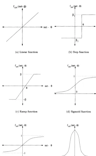
Frequently used activation functions are enumerated below:
1. Linear function (see Figure 2.2(a) for 0 = 0):
f AN (net -0)= ß(net - 0) (2.3)
The linear function produces a linearly modulated output, where ß is a con-stant.
2. Step function (see Figure 2.2(b) for 0 > 0):
fAN ( * n\ I ß1 if net >0 ,0 .v
2.2. ACTIVATION FUNCTIONS 19
fAN (net- 6)
-*~net- 6
net-(a) Linear function (b) Step function
fA N(net-6)
-*-
net-(c) Ramp function (d) Sigmoid function
fAN (net-6)
*•
net-fA N( n e t - e )
[image:42.468.58.376.79.595.2](e) Hyperbolic tangent function (f) Gaussian function
20 CHAPTER 2. THE ARTIFICIAL NEURON
The step function produces one of two scalar output values, depending on the value of the threshold 0. Usually, a binary output is produced for which ß = 1 and ß2 = 0; a bipolar output is also sometimes used where ß1 = 1 and
ß2= -!.
3. Ramp function (see Figure 2.2(c) for 0 > 0):
C ß if n e t - 0 > ß
fAN(net - 9) = net-0 if |net - 0| < ß (2.5)
[ -ft if net-0< -ft
The ramp function is a combination of the linear and step functions.
4. Sigmoid function (see Figure 2.2(d) for 0 = 0):
fAN(net -6)=
The sigmoid function is a continuous version of the ramp function, with
fA N(net) G (0,1). The parameter A controls the steepness of the function.
Usually, A = 1.
5. Hyperbolic tangent (see Figure 2.2(e) for 0 = 0):
e(net-0) _ e-(net-B)
fAN(net -0) =
or also defined as
fA N(net6) =
The output of the hyperbolic tangent is in the range (—1,1).
6. Gaussian function (see Figure 2.2(f) for 0 = 0):
fAN(net -0) = e-(net-0)2 (2.9)
where net — 0 is the mean and a1 the variance of the Gaussian distribution.
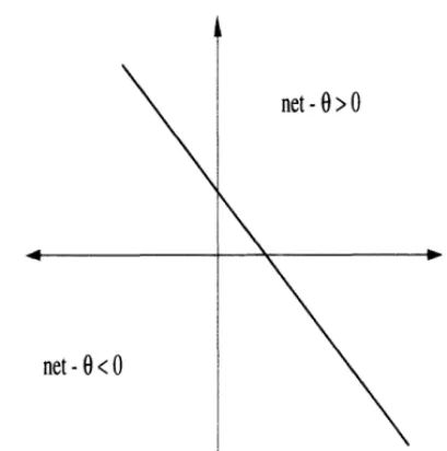
2.3 Artificial Neuron Geometry
Single neurons can be used to realize linearly separable functions without any error. Linear separability means that the neuron can separate the space of n-dimensional input vectors yielding an above-threshold response from those having a below-threshold response by an n-dimensional hyperplane. The hyperplane forms the boundary between the input vectors associated with the two output values. Fig-ure 2.3 illustrates the decision boundary for a neuron with the step activation func-tion. The hyperplane separates the input vectors for which ^i xiwi — 0 > 0 from
2.4. ARTIFICIAL NEURON LEARNING 21
net-0<0
net-0>0
[image:44.468.111.316.78.284.2]net-6 = 0
Figure 2.3: Artificial neuron boundary illustration
Thus, given the input signals and 0, the weight values wi, can easily be calculated.
To be able to learn functions that are not linearly separable, a layered NN of several neurons is required.
2.4 Artificial Neuron Learning
The question that now remains to be answered is, how do we get the values of the weights Wi and the threshold 91 For simple neurons implementing, for example, Boolean functions, it is easy to calculate these values. But suppose that we have no prior knowledge about the function - except for data - how do we get the Wi and
9 values? Through learning. The AN learns the best values for the wi and 9 from
the given data. Learning consists of adjusting weight and threshold values until a certain criterion (or several criteria) is (are) satisfied.
There are three main types of learning:
• Supervised learning, where the neuron (or NN) is provided with a data
set consisting of input vectors and a target (desired output) associated with each input vector. This data set is referred to as the training set. The aim of supervised training is then to adjust the weight values such that the error between the real output, y = f(net — 9), of the neuron and the target output,
22 CHAPTER 2. THE ARTIFICIAL NEURON
• Unsupervised learning, where the aim is to discover patterns or features
in the input data with no assistance from an external source. Unsupervised learning basically performs a clustering of the training patterns.
• Reinforcement learning, where the aim is to reward the neuron (or parts of
a NN) for good performance, and to penalize the neuron for bad performance.
Several learning rules have been developed for the different learning types. Be-fore continuing with these learning rules, we simplify our AN model by introducing augmented vectors.
2.4.1 Augmented Vectors
An artificial neuron is characterized by its weight vector W, threshold 0 and activa-tion funcactiva-tion. During learning, both the weights and the threshold are adapted. To simplify learning equations, we augment the input vector to include an additional input unit, xI+1, referred to as the bias unit. The value of xI+i is always -1, and the weight wI+1 serves as the value of the threshold. The net input signal to the
AN (assuming SUs) is then calculated as
net = ] xiwi +
i-l
i+i
= $>xiwi
i=1
where 9 =
In the case of the step function, an input vector yields an output of 1 when ES xiwi > 0, and 0 when
The rest of this chapter considers training of single neurons.
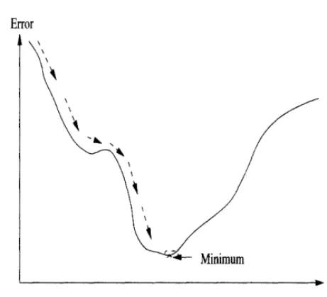
2.4.2 Gradient Descent Learning Rule
While gradient descent (GD) is not the first training rule for ANs, it is possibly the approach that is used most to train neurons (and NNs for that matter). GD requires the definition of an error (or objective) function to measure the neuron's error in approximating the target. The sum of squared errors
2.4. ARTIFICIAL NEURON LEARNING 23
is usually used, where tp and fp are respectively the target and actual output for
pattern p, and P is the total number of input-target vector pairs (patterns) in the training set.
The aim of GD is to find the weight values that minimize £. This is achieved by calculating the gradient of £ in weight space, and to move the weight vector along the negative gradient (as illustrated for a single weight in Figure 2.4).
Error
Minimum
[image:46.468.101.332.176.386.2]+ Weight
Figure 2.4: GD illustrated
Given a single training pattern, weights are updated using
with
where
38
df
(2.12)
(2.13)
(2.14)
and 77 is the learning rate (size of the steps taken in the negative direction of the gradient). The calculation of the partial derivative of f with respect to netp (the net
input for pattern p) presents a problem for all discontinuous activation functions, such as the step and ramp functions; xi,p is the i-th input signal corresponding to
24 CHAPTER 2. THE ARTIFICIAL NEURON
2.4.3 Widrow-Hoff Learning Rule
For the Widrow-Hoff learning rule [Widrow 1987], assume that f = netp. Then
= 1, giving
= _2(tp - fP)xiP (2.15)
Weights are then updated using
wi( t ) =wi(t-l)+ 2n(tp - fp)xi,p (2.16)
The Widrow-Hoff learning rule, also referred to as the least-means-square (LMS) algorithm, was one of the first algorithms used to train layered neural networks with multiple adaptive linear neurons. This network was commonly referred to as the Madaline [Widrow 1987, Widrow and Lehr 1990].
2.4.4 Generalized Delta Learning Rule
The generalized delta learning rule is a generalization of the Widrow-Hoff learning rule which assumes differentiable activation functions. Assume that the sigmoid function (from equation (2.6)) is used. Then,
onetp
giving
-^- = -2(tp - fp)fp(l - fp)xi p (2.18)
2.4.5 Error-Correction Learning Rule
For the error-correction learning rule it is assumed that binary-valued activation functions are used, for example, the step function. Weights are only adjusted when the neuron responds in error. That is, only when (tp — fp) = 1 or (tp — fp) = — 1,
are weights adjusted using equation (2.16).
2.5 Conclusion
2.6. ASSIGNMENTS 25
2.6 Assignments
1. Explain why the threshold 9 is necessary. What is the effect of 0, and what will the consequences be of not having a threshold?
2. Explain what the effects of weight changes are on the separating hyperplane.
3. Which of the following Boolean functions can be realized with a single neuron which implements a SU? Justify your answer.
(a) x
(b)
(c) x1 + x2
where x1x2 denotes x1 AND x2; x1 + x2 denotes x1 OR x2; x1 denotes
NOT xi,
4. Is it possible to use a single PU to learn problems which are not linearly separable?
5. Why is the error per pattern squared?
6. Can the function |tp — op| be used instead of (tp — op)2?
7. Is the following statement true or false: A single neuron can be used to
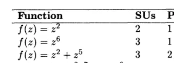
ap-proximate the function f ( z ) = z2? Justify your answer.
Chapter 3
Single neurons have limitations in the type of functions they can learn. A single neuron (implementing a SU) can be used to realize linearly separable functions only. As soon as functions that are not linearly separable need to be learned, a layered network of neurons is required. Training these layered networks is more complex than training a single neuron, and training can be supervised, unsupervised or through reinforcement. This chapter deals with supervised training.
Supervised learning requires a training set which consists of input vectors and a target vector associated with each input vector. The NN learner uses the target vector to determine how well it has learned, and to guide adjustments to weight values to reduce its overall error. This chapter considers different NN types that learn under supervision. These network types include standard multilayer NNs, functional link NNs, simple recurrent NNs, time-delay NNs and product unit NNs. We first describe these different architectures in Section 3.1. Different learning rules for supervised training are then discussed in Section 3.2. The chapter ends with a discussion on ensemble NNs in Section 3.4.
3.1 Neural Network Types
Various multilayer NN types have been developed. Feedforward NNs such as the standard multilayer NN, functional link NN and product unit NN receive external signals and simply propagate these signals through all the layers to obtain the result (output) of the NN. There are no feedback connections to previous layers. Recurrent NNs, on the other hand, have such feedback connections to model the temporal characteristics of the problem being learned. Time-delay NNs, on the other hand,
28 CHAPTER 3. SUPERVISED LEARNING NEURAL NETWORKS
memorize a window of previously observed patterns.
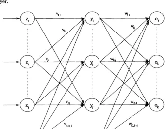
3.1.1 Feedforward Neural Networks
Figure 3.1 illustrates a standard feedforward neural network (FFNN), consisting of three layers: an output layer, a hidden layer and an output layer. While this figure illustrates only one hidden layer, a FFNN can have more than one hidden layer. However, it has been proved that FFNNs with monotonically increasing differen-tiable functions can approximate any continuous function with one hidden layer, provided that the hidden layer has enough hidden neurons [Hornik 1989]. A FFNN can also have direct (linear) connections between the input layer and the output layer.
Bias unit
Figure 3.1: Feedforward neural network
The output of a FFNN for any given input pattern p is calculated with a single forward pass through the network. For each output unit ok we have (assuming no
direct connections between the input and output layers),
[image:51.468.49.384.257.519.2]3.1. NEURAL NETWORK TYPES 29
J+i
J+l I+1
where fOk and fyi are respectively the activation function for output unit ok and
hidden unit yj; wkj is the weight between output unit ok and hidden unit yj; Zi,p
is the value of input unit Zi{ for input pattern p; the (I + l)-th input unit and the
( J + l)-th hidden unit are bias units representing the threshold values of neurons in the next layer.
Note that each activation function can be a different function. It is not necessary that all activation functions be the same. Also, each input unit can implement an activation function. It is usually assumed that inputs units have linear activation functions.
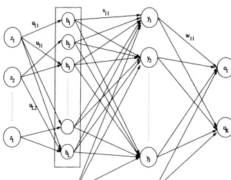
3.1.2 Functional Link Neural Networks
In functional link neural networks (FLNN) input units do implement activation functions. A FLNN is simply a FFNN with the input layer expanded into a layer of functional higher-order units [Ghosh and Shin 1992, Hussain et al. 1997]. The input layer, with dimension /, is therefore expanded to functional units h1, h2, - • • ,hL,
where L is the total number of functional units, and each functional unit hi is a function of the input parameter vector (z1, • • •, zI), i.e. hl( z1, • • •, zI) (see Figure 3.2).
The weight matrix U between the input layer and the layer of functional units is defined as
1 if functional unit hl is dependent of Zi ,„ ,
0 otherwise
For FLNNs, Vji is the weight between hidden unit yj and functional link hi.
Calculation of the activation of each output unit ok occurs in the same manner as
for FFNNs, except that the additional layer of functional units is taken into account:
J+l L
n, —f ok,P —
j=l 1=1
30 CHAPTER 3. SUPERVISED LEARNING NEURAL NETWORKS
Figure 3.2: Functional link neural network
3.1.3 Product Unit Neural Networks
Product unit neural networks (PUNN) have neurons which compute the weighted product of input signals, instead of a weighted sum [Durbin and Rumelhart 1989, Janson and Frenzel 1993, Leerink et al. 1995]. For product units, the net input is computed as given in equation (2.2).
Different PUNNs have been suggested. In one type each input unit is connected to SUs, and to a dedicated group of PUs. Another PUNN type has alternating layers of product and summation units. Due to the mathematical complexity of having PUs in more than one hidden layer, this section only illustrates the case for which just the hidden layer has PUs, and no SUs. The output layer has only SUs, and linear activation functions are assumed for all neurons in the network. Then, for each hidden unit yj, the net input to that hidden unit is (note that no bias is included)
TT
3.1. NEURAL NETWORK TYPES 31
= eE i vj i( zt,p) (3.3)
where Zijp is the activation value of input unit Zi, and vji is the weight between input
Zi and hidden unit yj.
An alternative to the above formulation of the net input signal for PUs is to include a "distortion" factor within the product, such as
where zI+1,P = — 1 for all patterns; vj,+1 represents the distortion factor. The
purpose of the distortion factor is to dynamically shape the activation function during training to more closely fit the shape of the true function represented by the training data.
If zi,p < 0, then zi,p can be written as the complex number zi,p = i2|Zi,p| (i = 1)
which, substituted in (3.3), yields
Let c = 0 + v = a + 6 be a complex number representing i. Then,
Inc - In rei° = Inr + i6 + 2nki (3.6)
where r = Aa2 + b2 — 1.
Considering only the main argument, arg(c), k; = 0 which implies that 2ki — 0. Furthermore, 9 = | for i = (0,1). Therefore, id = z|, which simplifies equation (3.9)tolnc=^ljr, and consequently,
Inz2 = z7r (3.7)
Substitution of (3.7) in (3.5) gives
7 7
^7r)] (3.8)
Leaving out the imaginary part ([Durbin and Rumelhart 1989] show that the added complexity of including the imaginary part does not help with increasing perfor-mance) ,
7
IbCLy- C 'r CUO^/l 7 Vji) V""*'/
32 CHAPTERS. SUPERVISED LEARNING NEURAL NETWORKS
Now, let
t=i
i=1
with
_/ 0 if zi
I 1 tf*K and Zitp / 0.
Then,
netyjp = ep>>p cos(7r<^)p) (3.13)
The output value for each output unit is then calculated as
J+i
f / X "* f / pj _ f sk \\ f 1 t A\
"Jfe,p — Joif \ }. ™kjjyj \€ COS^TTipjjjJ J v"--'-^/
Note that a bias is now included for each output unit.
3.1.4 Simple Recurrent Neural Networks
Simple recurrent neural networks (SRNN) have feedback connections which add the ability to also learn the temporal characteristics of the data set. Several different types of SRNNs have been developed, of which the Elman and Jordan SRNNs are simple extensions of FFNNs.
The Elman SRNN, as illustrated in Figure 3.3, makes a copy of the hidden layer, which is referred to as the context layer. The purpose of the context layer is to store the previous state of the hidden layer, i.e. the state of the hidden layer at the previous pattern presentation. The context layer serves as an extension of the input layer, feeding signals representing previous network states, to the hidden layer. The input vector is therefore
(3.15)
actual inputs context units
Context units zI+2, • • •, ZI+1+J are fully interconnected with all hidden units. The
connections from each hidden unit yj (for j = 1, • • •, J) to its corresponding context
3.1. NEURAL NETWORK TYPES 33
Context layer
Figure 3.3: Elman simple recurrent neural network
influence of previous states is weighted. Determining such weights adds additional complexity to the training step.
Each output unit's activation is then calculated as
J+i I+1+J
(3.16)
where (z1+2,P, • • •, zI+1+J,p) = (y1,P(t - 1), • • •, yj,p(t - 1)).
Jordan SRNNs, on the other hand, make a copy of the output layer instead of the hidden layer. The copy of the output layer, referred to as the state layer, extends the input layer to
z = (z1 , • • • , zIi+1 zI+2, • • • , zI+i+K (3.17)
actual inputs state units
The previous state of the output layer then also serves as input to the network. For each output unit we have
J+l I+l+K
34 CHAPTER 3. SUPERVISED LEARNING NEURAL NETWORKS
State layer
Figure 3.4: Jordan simple recurrent neural network
where (z/+2,P, • • •, zI+1+K,,p) = (01,p(t - 1), • • •, oK,P(t - 1)).
3.1.5 Time-Delay Neural Networks
A time-delay neural network (TDNN), also referred to as backpropagation-through-time, is a temporal network with its input patterns successively delayed in time. A single neuron with T time delays for each input unit is illustrated in Figure 3.5. This type of neuron is then used as a building block to construct a complete feedforward TDNN.
Initially, only Zi,p(t), with t = 0, has a value and zi,p(t — t') is zero for all i= 1, • • • ,I
with time steps t' = 1 , - - - , T ; T is the total number of time steps, or number of delayed patterns. Immediately after the first pattern is presented, and before presentation of the second pattern,
After presentation of t patterns and before the presentation of pattern t + 1,
/
all t — I. t,
3.1. NEURAL NETWORK TYPES
35Figure 3.5: A single time-delay neuron
This causes a total of T patterns to influence the updates of weight values, thus allowing the temporal characteristics to drive the shaping of the learned function. The connections between Zi,p(t — t ) and zi,p(t — t + 1) has a value of 1.
The output of a TDNN is calculated as
J+i I T
36 CHAPTERS. SUPERVISED LEARNING NEURAL NETWORKS
3.2 Supervised Learning Rules
Up to this point we have seen how NNs can be used to calculate an output value given an input pattern. This section explains approaches to train the NN such that the output of the network is an accurate approximation of the target values. First, the learning problem is explained, and then solutions are presented.
3.2.1 The Learning Problem
Consider a finite set of input-target pairs D = {dp = (zp, tp)|p = 1, • • • , P} sampled
from a stationary density £l(D), with Z,)P, t*)p € K for i = 1, • • • , 7 and k = 1, • • • , K ;
Zi,p is the value of input unit Zi and tk,p is the target value of output unit ok for
pattern p. According to the signal-plus-noise model,
tp = M£p)+Cp (3-19)
where (z) is the unknown function. The input values zi,p are sampled with
probabil-ity densprobabil-ity w(z), and the Ck,p are independent, identically distributed noise sampled
with density 0(0 5 having zero mean. The objective of learning is then to
approxi-mate the unknown function n(z) using the information contained in the finite data set D. For NN learning this is achieved by dividing the set D randomly into a training set DT, validation set DV and a test set DG. The approximation to n(z) is
found from the training set DT, memorization is determined from Dv (more about
this later), and the generalization accuracy is estimated from the test set DG (more
about this later).
Since prior knowledge about Q(D) is usually not known, a nonparametric regression approach is used by the NN learner to search through its hypothesis space H for a function FNN(DT', W) which gives a good estimation of the unknown function n(z),
where FNN G H. For multilayer NNs, the hypothesis space consists of all
functions realizable from the given network architecture as described by the weight vector W.
During learning, the function FNN : RI — >• Rk is found which minimizes the
empirical error
1 PT
ET(DT- W) = — V^yv^p, W) - -fp)2 (3.20)
PT^
where PT is the total number of training patterns. The hope is that a small empirical
(training) error will also give a small true error, or generalization error, defined as
3.2. SUPERVISED LEARNING RULES 37
For the purpose of NN learning, the empirical error in equation (3.20) is referred to as the objective function to be optimized by the optimization method. Sev-eral optimization algorithms for training NNs have been developed [Battiti 1992, Becker and Le Cun 1988, Duch and Korczak 1998]. These algorithms are grouped into two classes:
• Local optimization, where the algorithm may get stuck in a local optimum
without finding a global optimum. Gradient descent and scaled conjugate gradient are examples of local optimizers.
• Global optimization, where the algorithm searches for the global optimum
by employing mechanisms to search larger parts of the search space. Global optimizers include LeapFrog, simulated annealing, evolutionary computing and swarm optimization.
Local and global optimization techniques can be combined to form hybrid training algorithms.
Learning consists of adjusting weights until an acceptable empirical error has been reached. Two types of supervised learning algorithms exist, based on when weights are updated:
• Stochastic/online learning, where weights are adjusted after each pattern
presentation. In this case the next input pattern is selected randomly from the training set, to prevent any bias that may occur due to the order in which patterns occur in the training set.
• Batch/off-line learning, where weight changes are accumulated and used to
adjust weights only after all training patterns have been presented.
3.2.2 Gradient Descent Optimization
Gradient descent (GD) optimization has led to one of the most popular learning algorithms, namely backpropagation, developed by Werbos [Werbos 1974]. Learning iterations (one learning iteration is referred to as an epoch) consists of two phases:
1. Feedforward pass, which simply calculates the output value(s) of the NN
(as discussed in Section 3.1).
2. Backward propagation, which propagates an error signal back from the
38 CHAPTERS. SUPERVISED LEARNING NEURAL NETWORKS
Feedforward Neural Networks
Assume that the sum squared error (SSE) is used as the objective function. Then, for each pattern, p,
where K is the number of output units, and tk,p and Ok,p are respectively the target
and actual output values of the k-th output unit.
The rest of the derivations refer to an individual pattern. The pattern subscript,
p, is therefore omitted for notational convenience. Also assume sigmoid activation
functions in the hidden and output layers with augmented vectors. Then,
and
Weights are updated, in the case of stochastic learning, according to the following equations:
wkj(t) += wkj-(t) + ocj ( t - 1) (3.25)
Vji(t) += A«ji(*) + a&Vji(t - 1) (3.26)
where a is the momentum (discussed later).
In the rest of this section the equations for calculating Awkj(t) and Avj i(t) are
derived. The reference to time, £, is omitted for notational convenience.
From (3.23),
dok _ df0le _ .^ ^ , _ / (327)
dnet0le dnetOk k
and
Q J-t-1
where f'0k is the derivative of the corresponding activation function. Prom (3.27),
(3.28),
dot dok dnetn.
dnet0lc
= (1