Adaptive sampling in digital control

8-1964

Adaptive sampling in digital control

Kenneth Allen McCollom

Iowa State University R. M. Stewart Jr. Iowa State University

Follow this and additional works at:http://lib.dr.iastate.edu/ameslab_isreports Part of theElectrical and Computer Engineering Commons

This Report is brought to you for free and open access by the Ames Laboratory at Iowa State University Digital Repository. It has been accepted for inclusion in Ames Laboratory Technical Reports by an authorized administrator of Iowa State University Digital Repository. For more information, please [email protected].

Recommended Citation

Abstract

This study provides a set of design curves from which effective digital control for an experiment can be obtained and at the same time efficient use of a digital computer shared with other experiments can be realized. The state variable technique is used as both a design method for obtaining the design curves for adaptive sampling and for predicting the states for control of the process. The adaptive sampling technique is defined to be that choice of constant prediction period that will satisfy control specifications over a specified range of system conditions. The complete range of system operation is divided into a number of classes for which criteria can be devised for determining when the system is in each class. In each class the prediction period is no smaller than that required over the range of the operation of the class. The objective of the adaptive sampling is to use the digital computer for control as little as possible yet maintain the system control specifications.

Disciplines

Electrical and Computer Engineering | Engineering

IOWA STATE UNIVERSITY

ADAPTIVE SAMPLING IN DIGITAL CONTROL

by

Kenneth Allen McCollom & R. M. Stewart, Jr.

RESEARCH AND

DEVELOPMENT

REPORT

UNITED STATES ATOMIC ENERGY COMMISSION Research and Development Report

ADAPTIVE SAMPLING IN DIGITAL CONTROL

by

Kenneth Allen McCollom & R. M. Stewart, Jr.

August, 1964

Ames Laboratory at

Iowa State University of Science and Technology F. H. Spedding, Director

IS-995

This report is distributed according to the category Engineering and Equipment (UC-38) as listed in TID-4500, December l, 1964.

LEGAL NOTICE---,

This report was prepared as an account of Government sponsored work.

Neither the United States, nor the Commission, nor any person acting on behalf of the Commis sian:

A. Makes any warranty or representation, expressed or implied, with respect to the accuracy, completeness, or usefulness of the information contained in this report, or that the use of any information, apparatus, method, or process disclosed in this report may not infringe privately owned rights; or

B. Assumes any liabilities with respect to the use of, or for

damages resulting from the use of any information, apparatus, method, or process disclosed in this report.

As used in the above, "person acting on behalf of the Commission" includes any employee or contractor of the Commis sian, or employee of such contractor, to the extent that such employee or contractor of the Commission, or employee of such contractor prepares, disseminates, or provides access to, any information pursuant to his employment or contract with the Commission, or his employment with such contractor.

Printed in USA. Price $4. 00. Available from the Clearinghouse for Federal Scientific and Technical Information, National

Bureau of Standards, U. S. Department of Commerce, Springfield,

IS-995 CONTENTS ABSTRACT

I. INTRODUCTION

II. REVIEW OF LITERATURE III. METHOD OF INVESTIGATION

A. State Variable Technique 1. Recursion formula

2. Piecewise constant inputs B. Adaptive Sampling Technique

1. Prediction equations for unit block 2. Design parameters

C. Nonlinear, Time-varying Systems IV. EXPERIMENTAL IMPLEMENTATION

A. Description of Process System B. Derivation of Mathematical Model

1. Dynamics of sample radioactivity 2. Dynamics of sample transport

3. Dynamics of mass isotope separator 4. Combined dynamics at the target C. Solution for System Equations

D. System Control

1. Multilevel control equations 2. Application of adaptive sampling V. CONCLUSIONS AND RECOMMENDATIONS VI. BIBLIOGRAPHY

IS-995

ADAPTIVE SAMPLING IN DIGITAL CONTROL Kenneth Allen McCollom and R. M. Stewart, Jr.

ABSTRACT

This study provides a set of design curves from which effective digital control for an experiment can be obtained and at the same time efficient use of a digital computer shared with other experiments can be realized. The state variable technique is used as both a design method for obtaining the design curves for adaptive sampling and for predicting the states for control of the process. The adaptive sampling technique is defined to be that choice of constant prediction period that will satisfy control specifications over a specified range of system conditions. The complete range of system operation is divided into a number of classes for which criteria can be devised for determining when the system is in each class. In each class the prediction period is no smaller than that required over the range of the operation of the class. The objective of the adaptive sampling is to use the digital computer for control as little as possible yet maintain the system control specifications.

The method developed here is general enough to allow use by a con-trol engineer who has, or can develop, an adequate mathematical model for the process. The model is reduced to a set of first order differential

equations and then converted to Laplace Transform block diagrams. The knowledge of the behavior of a single first order differential equation, or similarly a single first order Laplace Transfer block, for a reasonable number of deterministic inputs allows the control engineer to analyze the control behavior of his complete block diagram one block at a time as sum-ing piecewise constant inputs to the block.

Using the method developed here, an interesting and useful charac-teristic is demonstrated for process systems which have particles or components that originate at the input of the process, are carried through the process in space and time and finally are expelled from the process never to return. These processes are commonly described by a set of nonlinear differential equations with time-varying coefficients. Solving this set of equations simultaneously is both a long and difficult task. For processes with the characteristics described above, this set of nonlinear differential equations can be uncoupled and the resulting sets solved in sequence. The experiment on which the adaptive sampling is demonstrated, the set of uncoupled equations prove to be individual first order differential equations that are linear.

jL,

.~

0o

J~,e__

Vr- a.-

Pn.

D.

~

2

~ ~

~

~~

4

.

~

.

~

{bju;J.J

tf6t/-k tL__

D~,~

f

~~ 'J~/

~-I. INTROD~CTION

Conventional automatic control has made significant

accomplishments in industrial and military applications. This type control is the design of control systems to determine the compensation necessary to fulfill a certain set of require-ments. The most common requirements are values of gain margin, phase margin, M-peak, rise time, settling time, peak overshoot, integral square error, and mean square error.

Pollowing many years of active development, conventional automatic control system design appears to be approaching a saturation point which, in turn, is encouraging the develop-ment of new theories of control. Perhaps the greatest impetus

for this change has been the computational aid supplied by modern digital computers. Some of the new mathematical techniques in the developing theories, such as dynamic pro-gramming, are impractical without the speed and capacity for calculations nov available.

The new techniques in control system design usually use the differential equations that describe the process mathemat-ically as a means for predicting what will happen in the

future. Then the predicted values are used to determine

usually the value of the variable in a first order

differen-tial equation describing a p~rtion of the process. If the

process is described by an nth order differential equation,

then it has n states which are normally determined in the

control problem.

The digital computer is not only aiding in the

develop-ment of such new theories but also is practically and, just

as important, economically implementing the theory by acting

as an element in the feedback loop of the control systems.

The economic advantage has resulted from two sources: first,

the cost of the computer hardware has declined to reasonable

values for use as control elements, and, second, the hardware

and software for computers has developed so that a single

computer can be shared by a number of different, otherwise

unrelated, experiments.

The purpose of this dissertation is to determine when

attention is necessary for the control of an experiment from

the computer which is shared with other experiments. To allow

investigation of the dynamic behavior of a process a unit

block which represents a first order differential equation has

been selected. Using deterministic inputs as driving

func-tions the characteristics of the unit block are determined for

a variety of inputs. A process system 1s investigated by

building up the complete system from the unit blocks. The

exactly with a piecewise constant input and approximately with

a time-varying input.

The error and deviation design curves for a number of

different deterministic inputs to the unit block are used in

the design of a multivariable control system for a nuclear

physics experiment. A sample is irradiated in a nuclear

reactorJ and the decay characteristics of the radioactive

atoms produced are examined. The sample is solidJ but through

controlled heating its vapor is continuously removed from the

reactor and inserted into the ion source of a mass isotope

separator. The mass isotope separator separates the

radio-active atoms from the parent atoms so that the decay

charac-teristics can be investigated. The control requirement is to

replace in a continuous stream from the reactor all atoms which

decay at the isotope separator target. The system is described

by a set of nonlinear differential equations with time-varying

coefficients and transport lags. The set of differential

equa-tions representing the system can be uncoupled to allow sequential

II. REVIEW 0!' LITERATURE

Prior to 1950, little was published in the area of

analysis and design of sampled-data systems. Digital

comput-ers were first used in control systems and later used in

complex automatic tracking systems for satellites in space.

The new emphasis on sampled-data systems has resulted in books

devoted solely to the subject (12, 16, 18, 19) instead of

chapters in the back of books otherwise devoted to continuous

control systems.

The design and synthesis of sampled-data control systems

can be divided into several categories. To aid in developing

the ideas for this dissertation, the categories here are

designated instantaneous feedback control systems and

predic-tive control systems. The instantaneous feedback control

system compares the present condition of the output to the

desired output and makes a correction to the system. The

pre-dictive control system, using the immediate system condition

and the expected inputs, predicts what the output will be at

some future time and makes a correction as soon as possible

following the calculations.

The instantaneous feedback control system was developed

first as sampled-data systems came into common use. The most

popular technique used to analyze these systems is the

for sampled-data systems is entirely analogous to the

applica-tion of the Laplace transformaapplica-tion to continuous-data systems.

Most of the techniques used for solving linear continuous-data

systems, such as the Nyquist criterion, root locus diagram or

Bode diagram, can be modified and extended to the studies of

linear sampled-data systems (12).

The predictive control systems predict the state of the

system at some future time using difference and state variable

equations derived from the differential equations describing

the physical system. In some sampled-data system design books

(16)

no distinction is made between the state of a difference

equation that is an approximation to the solution of the

dif-ferential equation and the state variable equation that is an

exact solution to the differential equation. A careful

docu-mentation of the history of the state variable method as

developed by both mathematicians and engineers has been made

by Fuller (5).

Kalman and Bertram (1~ have presented a general synthesis

procedure for using the state variable technique in the design

of a control system. However, the final control system uses

present values of the states for control of the system. Use

of the state variable technique in the design allows the

opti-mum choice of linear combination of all of the states to be

fed back to the input. Once these feedback terms are

controller. The authors do suggest that transport lags may be handled in the system using prediction. The digital computer is used for solving the prediction equations after each sample.

Dynamic programming theory applied to the optimum design of digital control systems (1, 2, 19) uses prediction by the

state variable method in a multistage decision process to

maximize the total return for a system. A systematic solution procedure may be derived by making use of Bellman's (1)

Principle of Optimality which states that "an optimal policy has the property that whatever the initial state and the

initial decisions are, the remaining decisions must constitute an optimal policy with regard to the state resulting from the first decision." This approach implies that to solve a speci-fic optimization problem the original problem is imbedded within a family of similar problems. The original multistage optimization problem is replaced by a sequence of single-stage decision processes which are easier to handle. The disadvan-tage is in checking all possible sequences of inputs to obtain the optimum one from each succeeding state. The number of possible paths increases with each succeeding stage.

Consid-erable computer storage is required to check every path and to allow a choice of the one which fits most satisfactorily the particular system.

using a two-level "bang-bang" type servo. The number of

possible branches of input sequences are reduced

consider-ably \'/hen only four inputs are available for choice. The

input variable operating-the controlled system is actuated

by an estimate of the error which will exist at some future

time. Repeated estimations of the future error are obtained

by predicting ahead1 on a fast time base, both the reference

and the controlled variable as well as some of their lower

order derivatives. The input signal is switched at the time

when the predicting computations determine that future

syn-chronization of reference and output w6uld occur if polarity

of the input signal were switched at that time.

The state of a linear system can theoretically be changed

to any other desired state by putting an impulse into the

state. Sufficient energy must be given by the impulse to the

system in zero time to change the state. Optimum control is

no longer a multistep requirement but can be obtained in a

single step at any time. Gupta and Hasdorff (6) have made the

technique practical by assuming that the input is a

combina-tion of a Gaussian (normal) shaped funccombina-tion and its

deriva-tives. The normal function in the limit as the standard

deviation goes to zero is the impulse function. With the

normal function the energy does not have to be delivered in

zero time. A basic difficulty is generating these normal

change the state is a function of the standard deviation which

is made as small as possible.

In many sampled-data control systems signals are sampled

periodically, although this type of sampling may not always be

possible and in some situations may not be desirable. The

introduction of aperiodic sampling may even improve the system

stability (12, p. 370). Recently a great increase of interest

has occurred in systems in which the sampling operations may

not be performed synchronously. Attempts have been made to

modify and use some of the methods for handling nonlinear

control systems such as describing functions or modifying the

Z-transform

(9).

These methods lead to complex analysis for

even simple systems.

Kalman and Bertram (11) have made a major contribution

in sampled-data analysis and control by showing how the state

variable technique can handle sampling systems of a general

type in a clear and uniform way. They claim that the method

yields simplifications even in the analysis and synthesis of

conventional periodic sampling systems. The method

auto-matically eliminates one of the chief difficulties of the

transform method, namely that it is difficult or cumbersome

to obtain information about the behavior of the system at any

time other than the sampling instants.

In their general theory, Kalman and Bertram give a very

as •a set

ot

numbers (called state variables) which contain as

much information regarding the past history of the element as

is required tor the calculation of the entire future behavior

of the element." The evolution of a dfnamic system through

time mar be visualized as a succession or state transitions.

Since each transition is independent of everrthing except the

present state and the input during the present transition,

then the non-uniform sample period is handled as easily as the

un1rora sample period. An important characteristic or the

state variable technique is that design effort is on the

analy-tical aspects of system problems with the drudger,y of

numeri-cal computations necessarily left to be performed by a digital

computer. The computations performed by the digital computer

after a sampling instant are usually quite short compared to

the time between two samples. Since this time is usually also

short compared to the time constants in the system dynamics,

the delay caused by the computations may be disregarded

alto-gather.

For simplicity, Kalman and Bertram use sample and hold

elements and assume that the input to the system is piecewise

constant. Any input that is var,ying can be integrated, if

known beforehand, through the convolution integral with the

transition matrix. The exact value of the input as a function

of time in the future must be known for this to be an exact

III. MEtHOD OJ INVESTIGATION

The extent to Which system design can proceed in a

logi-cal, systematic, and intelligent manner is to a degree

meas-ured by the knowledge of the process dynamics. Thus, the

first goal in control system design must be the determination

·of the dynamic characteristics of the process to be controlled.

The dynamic characterization of a process is commonly

de-scribed by a set of first order differential equations which

are functions explicitly of time and functions of the plant

states, x(t); driving control functions, u(t); and disturbance

functions, n(t).

In vector form,

~Ct)

=

1[

x(t), u(t), n(t), t

J

(1)

In addition to this general equation the process usually has

limits on the permissible driving functions because of

practi-cal considerations such as saturation or power limitation.

The mathematical model of a system may be made up of

differential equations with order greater than one.

Fortu-nately, equations of higher order can always be treated

numerically by reducing them to a larger system of first order

equations of the form of Equation 1. Henrici

(7)

has shown

that such reduction does not increase discretization error in

system equations to be first order, the model must first be

reduced to a first order set of differential equations.

A. State Variable Technique

The class of control systems which have received

con-siderable attention in the literature are those described by

the following vector form of the differential equations.

ict>

=

A(t)x(t) + u(t) + n(t) (2)

where A(t) is referred to as the coefficient matrix of the ·

process. This process is said to be linear and non-stationary.

However, the process is linear and stationary if A(t) is not a

function of ti.me. Por the latter case, consider the solution

to the homogeneous vector equation where there are no driving

functions or disturbances to the system. Thus

i(t)

=

A i(t) (3)

rhe plant starts to move at time, t0 , from an initial state,

X •

0 The solution of this homogeneous vector differential equation is similar to the solution of a single first order

differential equation

x(t)

=

m x(t) (4)

m(t-t0 )

x(t)

=

e x0 (5)

where m is a constant. In the vector differential Equation 3

the term, A, is a matrix. Before a solution of the vector

differential equation can be obtained by analogy to the first

order differential equation a definition of exponentiation of

a matrix must be made. Since

(X)

emt

L

mktk

=

_~ (6)

k=O

then let

(X)

eAt

₌

L

Aktk

kT""

(7)

k=O

for which there are defined matrix operations. This suggests

that the solution for the vector differential equation is

i(t)

(8)

The equation

(9)

is commonly defined as the transition matrix of the system

since

shows that if i ₀ are the states at some initial time, t0 , the

movement or transition of the states to new positions at t is

only a function of the initial state and the transition matrix.

The solution of the general differential equation with

driving forces and disturbances can be shown to be of the form

(11)

Differentiating with respect to t gives

-• •

x(t) =A x(t) + •<t - t0)01 (t) (12)

Setting this equal to the general form of the differential

equation in Equation 2 with A not being a function of time

makes the following equality necessarr tor Equation 11 to be

a solution.

-

•

A i(t) + u(t) + n(t) =A i(t) + •<t - t₀)o_1(t) (13)

Cancelling terms and solving for

W

_{1(t) gives}

Substituting this into lquation ll givea the aolut1on aa

i'(t)

the intecral sign since it is not a tunction of the

integrat-iDC Yariable. The definition of the transition matrix as an

exponential function allows consolidation ot the two

transi-tion matrices now under the integral sign. In additransi-tion, at

t

=

t0 the transition matrix, •<t - t0 ), becomes the identity

matrix. Therefore the constant 02 is just the value of x(t0 ). fhe final result is

where

and the vector form of the equation tor which this is the

solution is

....

(17)

x (

t )

=

A % ( t) +

u (

t ) + i ( t ) ( 18 )

the linear, tima-stationar.y form of lquation 2. This powerful

equation expresses the instantaneous motion of the process in

terms of the driving control signals, aD7 disturbances and the

initial states. !hese equations describe the exact motion of

the process if the original equations are an exact

mathemati-cal model of the process and if the control signal, the other

driving functions and the disturbances are exactl7 known.

on the results. The exactness of this solution is emphasized

since the approximate numerical solution of a differential

equation is often obtained by solving a related difference

equation which results in -a state-transition equation similar

to Equation 16.

1. Recursion formula

The state variable solution developed in the last section

and shov.n 1n Equation 16 is more useful tor handling in the

computer if the equation is placed in a recursive form. This

can be accomplished if the prediction period is constant.

Disturbances also a~e assumed to be zero and all inputs are

assumed to be deterministic in nature.

Letting the present time be tk and eliminating the

disturbance term as an input to the system, Equation 16

be-comes

This general form, valid for t > tlt, is usefUl for calculating

exact output states where more than one stage is in sequence.

However, the recursion equation is obtained b7 alwa7s

predict-ing a fixed period, T, ahead

ot

the present tiae. !hua, if t

(20)

The following substitution will be useful throughout:

(21)

Equation 20 is the equation with which the majority of the

future development is involved.

The recursion formula can be used· for two different

situations that appear in control systems. When the

differ-ential equations describing the dynamics of the system are

reduced to a set of first order differential equations and

states assigned, all of the states will probably not be

measurable. If ~~e state cannot be measured, the value of

the state at the present is known only through having

calcu-lated it in the prediction Equation 20, starting from a known

initial condition of the state. Thus, any error in predicting

the state T seconds later tends to accumulate as any transient

condition persists. A state that cannot be measured is

re-ferred to as an inaccessible state, and the state that is

measurable is an accessible state. Usually, through careful

choice of states, most of the state variables in a system can

be measured. Accessibility and inaccessibility are fundamental

to the application of the state variable method, since the

method requires that the present state be known. Any error in

a transient input condition and disappear during a stable

input condition to the state.

Referring again to the recursion Equation 20, the

dif-ference in using this equation for calculation of the

acces-sible and the inaccesacces-sible states is the value used for

x(tk). If the state is accessible, the value of the

measure-ment at tk for the state variable is used. If the state is

inaccessible the previously predicted value for the state is

used. The predicted values for the states x(tk+l) just T

seconds later are exact values only if both the present states

x(tk) are known and the driving functions u(t) are known for

the period.

2. Piecewise constant inputs

The state variable technique offers the control engineer

a set of tools which allows him to predict the complete state

of his process at any future time. The prediction is exact

only if he knows the input driving functions to the process

from the present to the time of the prediction. If the

driv-ing function is under his control, he has no problem. However,

there are driving functions that are not under his control and

can change at any time. To allow prediction to still be

accomplished some type of approximation for the input over the

sample period must be made.

driving function remains constant during T in Equation 20. A

more sophisticated procedure is to linearly extrapolate the

driving function from its value at the preceding time through

the value at the initial time and on to a value at the

predic-tion time. An even more intricate procedure is to curve fit

the last three input function values and represent the driving

function as a polynomial. The last two procedures require

considerable computer processing which for a real-time, shared

computer could be impractical.

The mathematical form is most simple when the driving

functions for a given differential equation in the matrix are

measured and are assumed to remain constant at that value over

the period of prediction. The amount of error is dependent on

how far the driving function changes during the period. By

investigating the system it is usually possible to determine

how rapidly a driving function can change. For example, if

the input to a given differential equation is the output from

another state of the system, the time constant for that state,

together w1 th its permissible inp·ut, will limit the rate of

magnitude change possible. Chemical reactions can only

pro-gress at certain rates which can be measured and defined. In

the system to be considered later, the neutron flux in the

reactor will normally change no faster th.an a certain

pre-scribed rate.

remains constant can be investigated. The results can

deter-mine the time available for prediction and error correction

without exceeding the control specifications of the system.

One fortunate conditicn exists for the general prediction

equation. If the driving function remains constant for several

periods, any past errors gradually are reduced to zero. This

condition fits nicely the intuitive idea that the most recent

measurements should be the ones that more readily indicate the

value of the present state and that the measurements made in

the more distant past have less and less weight on the value

ot

the present state. Then, if there are no calculation

errors for a period. of time, the total error diminishes.

Choosing the simple approximation of a piecewise constant

driVing function to all differential equations in the system

simplifies the control computations required from the digital

computer to a minimum number of simple manipulations.

B. Adaptive Sampling Technique

An adaptive sampling technique is here defined to be that

choice of constant prediction period that will satistJ S,Jstem

control specifications over a specified range of systea

condi-tions. The complete range of system operation is divided into

a number of classes for which criteria can be devised for

the prediction period is to be no smaller than that required

over the range of the operation of the class. The objective

for the adaptive sampling is to use the digital computer for

control as little as possible yet maintain the system control

specifications.

A method is developed here that is general enough to

allow use by a control engineer.who has, or can develop, an

adequate mathematical model for the process. The model is

reduced to a set of first order differential equations and

then converted to Laplace Transform block diagrams. The

knowledge of the behavior of a single first order differential

equation, or similarly a single first order Laplace Transform

block, for a reasonable number of deterministic inputs allows

the control engineer to analyze the control behavior of his

complete block diagram one block at a time.

The first order differential equation to be used as the

basic building block is given by

(22)

and the corresponding Laplace Transform unit block is shown in

Figure l. A set of deterministic inputs are also shown in

Figure l. The equations representing these inputs are

Positive exponential:

Unit step w1 th

negative exponential:

(25}

(26}

Since the differential equation is a linear equation, the

principle of .superposition applies. The total response of the output for the sum of several inputs at the same time is found by considering each input separately and swaming their

indi-vidual outputs. This allows even more variety in simulating different inputs.

1. Prediction equations ~ ~ block

Two sets of prediction equations are required to allow development of design parameters for decisions for the adap-tive sampling. One of the sets of equations is an exact solution for the output of the unit block for a given input. The other set of equations is that which uses piecewise con-stant approximations for the input and thus obtains an approx-imate solution for the output of the unit block. fhis set of equations will later be used as the control equations in the real time digital control. In this section, the approximate solutions are compared to the exact solutions for a given input to generate design parameter curves.

The recursion equation developed earlier and given in

u1( t )

block are obtained. For the first order differential equation

given in Equation 22, the transition matrix is readily

deter-mined from the homogeneous solution to be

(27)

Substituting this into the recursion equation gives

... _

This equation generates both the exact and the ~pproximate

solution for the output when u1 (t) and u1 (tk)' respectively, are used for u1 ( T) ·under the integral sign. In the

approxi-mate case, u1(tk) is no longer a function of the integrating variable, so it can be brought out in front of the integral

sign. In _{the exact case u1 is a function}

ot

the integrating

variable so cannot be brought outside of the integral.

The simulation of the unit block is made ld.th IC and all

inputs set to unity. This allova universal curves to be

generated with gain factors inserted b7 the deSign engineer

for each s7stem investigated. The percent error used for the

exponential curves is defined b7

(29)

automatically normalizes the result since all gain factors

cancel. The inputs other than the exponential ones use the

deviation between the exact and the approximate outputs to

allow the generation of useful design curves.

Initiating each of the inputs at the instant of a sample

tends to maximize the error presented in the resulting curves.

Anytime there has been a choice of doing part of the

measure-ment or calculation two ways, the one causing the most error

has been chosen. The resulting curves tend to be pessimistic

in their estimate of the error. In the case·of the unit step,

there is only error in predicting the output between the time

the step occurs and the next sample instant, since after that

the input is constant. A constant input makes the output

prediction for both the approximate and the exact solutions

identical.

The prediction equations are obtained by substituting

u1 (t) and u1 (tk), respectively, for each input investigated. Integrating over the recursive limits gives the following set

of recursive prediction equa tiona. for the unit block transfer

function shown in ligure 1:

Case a: u1 (t)

=

t, u1 (t0 )

=

0, x1 (t0 )

=

0

Approximate solution

Exact solution,

-(l-n)T/-r1

:x₁(t_{1 )}

=

l - e

t/Tp

Case c: u1 (t)

=

e , _{u1 (t}0 )

=

1, x1 (t0 )

=

1

Exact solution,

Approximate solution,

(31)

(32)

-T/Tl

e )

(33)

-T/Tl kT/Tp -T/Tl

xl(tk+l)

=

e x

₁

(tk) + e

(1 -

e )

(34)

Case d: . _{u1 (t)}

=

e -t/T P, u1(t~)

=

0, _{u1 (t}+ _{0 )}

=

1, x_{1 (t}0 )

=

0

Exact solution,

-T/Tl

e )

(35)

2. Design parameters

The recursion equations describing the exact solution and

the approximate solution of the output state for the four

input cases are placed in forms that minimize the number of

variables. Wherever possible, the sample period and the time

constants, T, were put in ratio form, T/T. This is a

non-dimensional ratio which is easy to use in the general

applica-tion of these curves. · The abscissa of each of the curves

generated has been made the ratio of the sample period to the

time constant of the unit block, T/T_{1 .} The ordinate is either some form of the percent error or the deviation of the

approx-imate value from the exact value of the output state. Finally,

the family of curves is generated by the remaining variables

in each of the cases. For instance, in all of the exponential

inputs, the families of curves are for different values of the

ratio of the unit block time constant to the exponential time

constant, T1/Tp·

The approximate solution may have either ~ accessible or

an inaccessible output. If the output is accessible, then the

present state, x1(tk), of the system is obtained from the

exact solution when prediction was made from the previous

state. The exact solution gives the same result as a

measure-ment does for the present state. If the output is

inaccessi-ble, then the present state, x₁(tk), is obtained from having

The ramp input to the unit block

eventually results in a fixed amplitude deviation between the

approximate output and the exact output for a given sample

period. The time in Which the deviation ceases to increase

is dependent upon the time constant of the unit block, T1 • Since the abscissa of the curves is !/T1 a family of curves shows the gradual increase in amplitude at each tk following

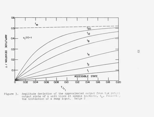
the initiation of' the ramp. ?igures 2 and 3 show two

differ-ent scales for the abscissa and d1splaJ the deviation of' the

approximate output from the exact output. The curves

desig-nated as tk show the deViation at the end of the kth period

just kT seconds after ~n1t1at1on ot the ramp. Por the

acces-sible case, the deViation is reduced to zero again at the end

of each period by a measurement. The result is that the

deViation at the next sample is again the same value as shown

at t 1 for a given value of T/T1 • !hus, onlr one curve, that designated t 1,is used for the aooeslible output state, while all of the curves are used for the inaccessible output state,

and the deviation at lt! seconds ia indicated b7 the curve

designated as ~· A daShed line in both of the figures

indi-cates the asymptotic value of the deYiation at t00 • Since the

simulation in the digital ooaputer was carried onlr to ·lt

=

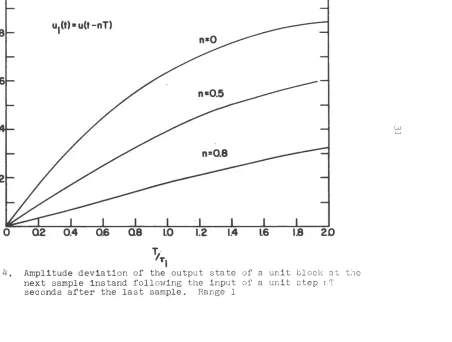
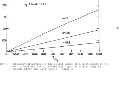
20, further specific curves are not included.

b. u1(t)

=

u(t - nT) The unit step input to the unit block results in a deviation ot the output state at the next

J> ~

,

c

2

0 fTI

0 fTI

<

~

0 u1 (t)•t.

[image:36.593.75.725.45.519.2]

z _{0 .} ...

-t _{ACCESSII..E STATE}

0

2.0

~

_Tl

Figure 2. Amplitude deviation of the approximated output from the actual output state of a unit block at sample instants, tk, followitig the initiation of a ramp input. Range 1

1\)

0.

---tCI)

- - - , 2 0

_____ _

---

-

---)>

~

,

u₁(t)=t

c

c!

0

1"1

0

1"1

<

~

[image:37.587.63.628.47.532.2]

~ ...

-i

0.20

T/.

TJ

Figure 3. Amplitude deviation of the approximated output from the actual

output state of a unit block at sample instants, tk' follol'lilJ:_:;

the initiation of a ramp input. Range 2

constant

ot

the unit block. As the sample period is made

longer, the output has time to grow larger. The deviation, as

a function of T/T 1 and the time after a sample that the step starts, is shown for

twn

_{ranges of T/T 1 in Figures 4 and 5.}

The parameter, n, varies between 0 and 1 where the step occurs

at t~ for n

=

0 and at ti for n

=

1. As previously indicated,

there is no .further deviation between the approximate solution

and exact solution for the output after the first sample

following the unit step.

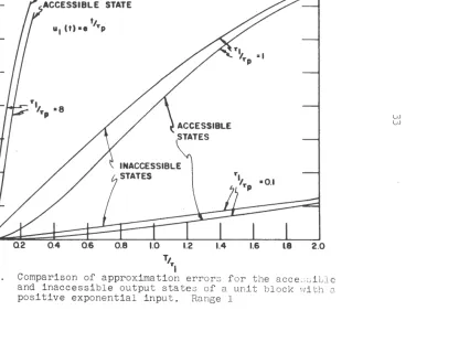
c. ul(t)

=

et/Tp The positive exponential input to

the unit block eventually results in a constant error between

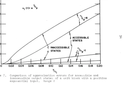
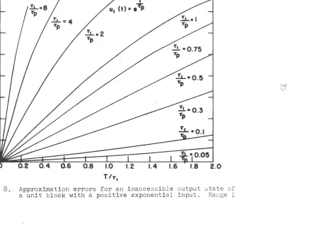
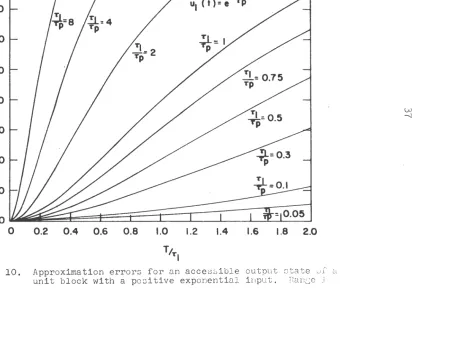
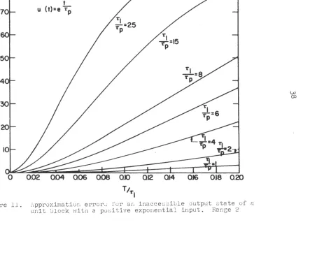
the approximate output and the exact output for given T/T 1 and T1/Tp· The exponential input reaches this asymptotic error in a time dependent on the time constant of the unit block.

Since the abscissa is in terms of T/T 1, the small values of the abscissa take more sample periods to reach the asymptotic

error. For T/T 1 greater than 0.5 the asymptotic error is reached in three or four sample periods. The comparisons for

the asymptotic errors, resulting for the inaccessible and

accessible output states, are shown for two ranges of T/T 1 in Figures

6

and

7.

These two figures are included for

compara-tive purposes only. The inaccessible state for two ranges of

T/T 1 and a more complete selection of ratios, T_{1/Tp' are given}

in Figures 8 and 9. Similarly, the accessible output state is

I

~

~

0

"'

₀

~

i

'

....

!4

-u₁ (t) • u(t -n T)

0.

T· ~TI

n•0.5

n=0.8

[image:39.591.139.645.106.518.2]

20

Figure

4.

Amplitude deviation of the output state of a unit bl ock at the

next sample instand following the input of a unit step r:T

seconds after the last sampl e. Range 1

\.AJ

~

,

r

-t

c

c

""

c

1"1

<

~

0

z

...

-t

~

-u1 (t)= u(t-nT)

n=O

0~~~~~~~~~~

[image:40.591.130.689.117.478.2]

T/ Tl

Figure 5. Amplitude deviation of the output state of a unit block at the

next sample instant following the input of a unit step nT

seconds after the last sample. Range 2

l.JJ

•

en

-<

c

.,

~

0

ITI

::u ::u

0

::u

I

.,

ITI ~ ITI

z

~

02

INACCESSIBLE STATE

ACCESSIBLE STATE

Ul (t) ae f/Tp

0.4 0.6 2.0

[image:41.593.177.623.120.498.2]

~ ~

Figure 6. Comparison of approximation errors for the accesGilJle

and inaccessible output states of a unit block wi th a positive exponential input. Range 1

•

(I) ~ E

.,

~

~

0

"'

::u ::u

0

::u

•

.,

"'

::u n

"'

z ~

6

0

'"

ul (t)• e "p

0.02 0.04 . 0.06 008

INACCESSIBLE STATES

0.10

T

,,.

,

OJ2 0.14 OJ& 0.18 0.20

Figure

7.

Comparison of approximation errors for accessible and

inaccessible output states of a unit block with a positive

exponential input. Range 2

LU

[image:42.591.147.641.106.479.2]

+:-en

-<

c

,

-t

0

-t

-

n

"'

:a

:a

0 ~

I

.,

"'

~

n

"'

z

-t

[image:43.593.139.610.103.505.2]

TITI

Figure

8.

Approximation errors for an inaccessible output state of

a unit block with a positive exponential input. Range 1

VJ

l>

(/) -<

3:

"'U

~

0

rTI

::u ::u

0 _{"2,.j_} ::u

I

"'U

rTI

::u 0

rTI

z

---4

I

/

/

T

/TI

To~ _j

020

Figure S,. .\pproximatior; error e; i:cr c'i1 inacce~ot>ii.Jle output state __ r·

unit bl oclc ui tn a po ~;i t i ve exponential i!<pu t. Range 2

w

)>

(J)

70

-< 60

~

.,

-t

~ 50

0

,

:u

::0

0

:u

40

30

~ 20

::0 0

,

z 10

-t

u1 ( t) = e Tp

o

!U/~

1 1

C

1 1

if=,o.o5]

0 0.2 0.4 0.6 0.8 1.0 1.2 1.4 1.6 1.8 2.0

[image:45.593.132.610.108.493.2]

TtTI

Figure 10. Approximation errors for an accessible output state 01 ct

unit block with a positive exponential input. nar1se 1

l.AJ

l> ~

3:

~

0

1"1

:::u

~

:::u

I

,

1"1

:::u

~

~

0

t

u (t)=e TP

0.02 0.04 0.06 0.08 0.10

TtT

I

Ql6 _{OJ8 0.20}

Figure 11. Approximation error0 for ar; inaccessible output state of n

unit block with a positive exponential input. Range 2

w

[image:46.600.127.631.88.494.2]

general way the error at early sample periods prior to

reach-ing the asymptotic error. However, the comparison of the

accessible and inaccessible output states may prove useful,

and it is true that the error l s alwc1ys smaller than the

asymptotic value in the earlier sample periods. -tl-r

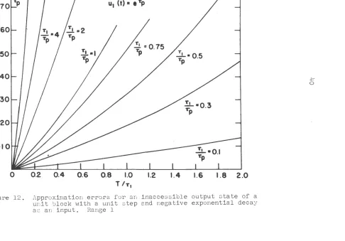
d. u1(t)

=

e 1 P The unit step followed by an

exponentialiy decreasing decay has characteristics quite

similar to that of the positive exponential. Two

character-istics are different. First, the error ls negative. The

decay makes the approximate solution for the. output state have an input that is always equal to the exact input at the sample

instant, but at al~ other times the input is greater. From

the error definition of Equation 29, the error is negative.

Second, an interesting result from this input is that the

error is constant from the very first sample for the

inacces-sible state. The error, then, does not have to be called an

asymptotic error since it is constant as a function of time.

The curves for two ranges of T/-r 1 for the inaccessible case

are shown in Figures 12 and 15. The results for the accessi- ·

ble case did not reduce to conditions that could be

meaning-fully displayed on a graph. At the first sample, the error

was the same as that for the 1nacoessi ble case.. After· that, the error decreased continually for the twenty samples

simu-lated on the computer. For this type of input, then, the

1"1

::0 ::0

0

::0

I

,

,.,.

::0

0

1"1

z

-t

0.6 0.8 1.0 TIT,

1.2 1.4

!L.o

.3

T"p

[image:48.595.102.588.113.504.2]

1.6 1.8 2.0

Figure 12. Approximation errors for an inaccessible output otate of a

unit block with a unit step 2nd negative exponential decay

as an input. Range l

SJ

:::0

~

I

~

~

~

. -i

t u₁ (t)•e- T"p

T/.

Tl

[image:49.599.72.617.79.504.2]

0.20

Figure

13.

Approximation errors for an inaccessible output state of u

unit block with a unit step and negative exponential decay

as an input. Range 2

C. Nonlinear, Time-varying Systems

The previous discussion has been limited to linear, time invariant processes. Unfortunately for the control engineer these characteristics seldom exist. If a linear approximation is used to describe a process that is not linear or time

stationary, the major question is the validity of the

approxi-mation.

Considering Equation 2 again, the transition matrix is

now a function of time and the initial time, t_{0 •} The general form would be ~(t, t0 ) instead of that obtained in the linear

case ~{t - t_{0 ).} Even though ~{t, t_{0 )} can also be expressed as an exponential as in the time-invariant system, the result is not nearly as satisfactory. There results no formula for +(t, t_{0 ),} although Tou (19) indicates that the transition

matrix can be expressed as an infinite series of successive integrals. This is not a convenient form with which to work,

and general procedures to derive the transition matrix apparently have not yet been obtained.

A non-linearity found in many processes shows up as a product of two of the state variables in the set of first

order differential equations describing the plant. Solutions for values of some of the states are needed before all equa-tions can be solved. A simultaneous matrix solution can only

to the correct values ·for the states. There are obvious computing time disadvantages of an iterative procedure for a

real-time shared digital computer for system control.

There is a type of plant that can be described by a set of first order differential equations which, in matrix form,

can be reduced in order and thus simplified. In general, this system is one that has parts of the system separated in space from other parts. In a continuous chemical plant the solution may pass through one tank with a catalyst which will cause a

certain reaction to take place. When the solution leaves that tank and proceeds to the next step the reaction will stop

be-cause of absence of the catalyst. Mathematically this part of

the system can be described by an independent sub-set of the set of equations describing the complete plant. The sub-set

can be solved first and the results inserted into the rest of

the equations. An example considered in Section IV uses a nuclear reactor as a source of neutrons to activate a

radio-isotope. No more radioactive isotopes are produced ~en the

sample is removed from the reactor enviroDaent. S1m1larly, a mass isotope separator is used to separate t.he sample stream. The behavior of the separator and its controls has no effect

on the production of the radioactive nuclides in the reactor.

These, then, are independent sets of equations and should be

able to be solved independently of the complete set.

set of equations is that one of the states involved in a

product of state variables may be in an independent sub-set of

the equations. As a consequence, the state can be determined

and act as a constant, and the non-linearity is removed. The

tool is convenient for use on such non-linear equations.

The independent sub-sets of the complete set are easily

recognized when the equations are put in matrix form. If a

q x q block of elements is found in the coefficient matrix

with all other elements in the q rows being zero, then these

q equations are independent of the other equations in the

matrix. One caution is that the driving functions must be

checked to see that no states or controls from outside the q

rows are encountered. Since the set of first order

differ-ential equations describing the system can be placed in any

sequence to make up the matrix, the best combination of zero

elements in the reduction of the order of the matrix can be

IV. EXPERIMENTAL IMPLEMENTATION

The adaptive sampling technique using state variable

prediction for control has been used in the design of a

con-trol system for an experiment in a nuclear reactor. The

purpose of the experiment is to investigate the decay schemes

of radioisotopes continuously produced and removed from the

reactor at a rate approximately equal to the half life of the

particular radioisotope. The effect is to produce a

radio-isotope with an infinite lifetime. The purpose of the control

system is to maintain the rate of arrival of the radioactive

atoms equal to the rate of decay from the isotope target.

A. Description of Process System

A schematic representation of the system is shown in

Figure 14. The nuclear reactor core provides a source of

neutrons when the reactor is operating. These neutrons are

in close association with a sample in a nearby experimental

facility and thus turn a certain portion of the atoms into

'

radioactive atoms by neutron capture. The solid sample is

contained in a chamber that is at a high vacuum and is

vaporized at a controlled rate by a heater. The vapor flows

out of the chamber in the reactor through a tube approximately

I

I

/

I

I

Sample Heater Current

Ion Source Magnet-...,

on Source lament

.Current

•~---Ion Accelerating and

Isotope-._.." Separator Magnet

Focusing Electrodes

[image:54.591.115.512.58.610.2]

Target

this transfer line. The ion source ionizes the sample vapor

and accelerates the resulting ions through a constant

poten-tial into the magnetic field of the separator. The separator

allows isotopes with different masses to be collected at

dif-ferent physical locations in the plane of the target at the

receiving end. At this point the physicist may examine the

radioisotopes that have been produced with the appropriate

physical tools.

The sample is usually non-radioactive when inserted into

the reactor. The buildup of radioactivity depends on the time

history of the neutron flux in the reactor, the neutron

capture cross section of the atoms and the half life or decay

constant of the radioactive nuclides. The vapor from the

heated sample will gradually build a pressure that will cause

other vaporized atoms to be transported down the line and into

the lower pressure area of the ion source and mass isotope

separator. The vapor enters a plasma in the ion source that

..

is sustained there by a filamentary heating elaent, a magnetic

field and appropriate element potentials. fhe vapor·beoames

ionized When encountering the high temperature of the plaaaa.

A small opening at the end of the ion source, beyond whiCh are

located appropriate extracting, accelerating and focusing lens

potentials, allows continuous extraction and acceleration of a

accelerated into the magnetic field of the mass isotope

separator, and the curvature of the beam along its flight path

in the field depends on the mass of the ions. The parent atom

normally captures one neutron to form the radioactive daughter

atom just one mass unit heavier. The parent and daughter

atoms can be separated sufficiently in space to allow separate

manipulation by the experimentalist. This action is similar

to that in a mass spectrometer used to identify different

atomic masses in analytical measurements, except that the mass

isotope separator provides a sufficient quantity of atoms to

allow physical or chemical experiments. A simplified word

block diagram shown in Figure 15 gives a reasonable flow

dia-gram of the interactions that take place in the process.

B. Derivation of Mathematical Model

The process system naturally divides into three parts

for studying its mathematical character: the first is forming

of radioactive atoms in the sample; the second is producing

vapor from the solid sample and transporting the vapor to the

inlet of the ion source of the mass isotope separator; the

third is converting the non-ionized sample to an ionized form

in the ion source and accelerating it through the separator

magnetic field to a target. The first objective will be to

Power to sample heater

I

Pressure in radiation volume

Transport lag

Aps

Total current in isotope separator

Power to ion source filament

IT

1--Neutron flux at sample

Radioactive atoms in

sample

Transport lag

N

M

Radioactive part I R B

-L.o_f_i_s_o_t_o_p_e_s_e_p_a_-_,..._ Target rator current

Decay rate

J1gure 15. Word flow block diagram of important variables in the experiment

adequately describe the complete process system and the

interactions between the variables.

1. pynamics

2f

sample radioactivity

The differential equations that describe the behavior of

a sample in neutron flux are well worked out in the literature

(8).

The two equations that describe the process for this

system are

dN(t) __ N(t) M( )d(t) N(t) w(t)

(37)

dt - A + ~ t P - N(t) + M(t)

dM(t) __ ~ M(t)¢(t) _ Mtt) w(t)

~ - N( ) + M(t)

where N(t)

=

number of radioactive atoms at any time,

M(t)

=

number of parent atoms at any time,

¢(t)

=

neutron flux, neutrons/cm2-sec,

(38)

~

=

neutron capture cross section of the sample, cm2

'

A

=

decay constant of the sample, sec-1 ,

t

=

time, sees, and

w(t)

=

flow of vaporized atoms, atoms/sec.

In Equation

37

the first term on the right is the rate of

disappearance of radioactive atoms by decay, the second term

is the rate of appearance of new radioactive atoms from

cap-ture of neutrons, and the third term is the rate of

transport-ing away the solid sample. In Equation 38 the first term is

the rate of disappearance of the parent atoms due to the

form-ing of radioactive atoms, ~d the second term is the rate of

disappearance due to transporting away the vaporized sample.

Several approximations for these equations are

appropri-ate when the conditions of the irradiations and the particular

samples used in this system are considered. It is expected

that a sample will seldom be smaller than 100 grams which is

approximately 1025 atoms of the parent. The maximum

vaporiza-tion rate that can be tolerated as an input to the mass

iso-tope separator is approximately lo15 atoms/second. Of this

total vaporization.rate the number that will be radioactive

is no greater than 109 atoms/second for the half lives,

neutron flux and sample cross sections involved. Thus, the

ratio N/M is no greater than lo-6 • In Equation 38 both terms

are negligible compared to the other time constants in the

system. Thus M(t) is no longer a function of time but rather

a constant equal to the total sample. In the case of a sample

that is very small or a combination of a very mull sample and

a long irradiation time, this approximation is no longer true,

and the second differential equation must be considered to

give a complete description of the system.

In Equation 37 the rate of change of the number of

active atoms in the sample due to vaporization of the