Real-time Visual Flow Algorithms for
Robotic Applications
Juan David Adarve Bermudez
A thesis submitted for the degree of
Doctor of Philosophy
The Australian National University
Except where otherwise indicated, this thesis is my own original work.
Acknowledgments
This thesis has been the work of many years and several (many) steps in the wrong direction. Throughout the journey, I have learned the meaning of doing quality research and to think about some fundamental questions currently important in robotics. None of this would have been possible without the guidance of Robert Mahony, my mentor and supervisor. Our regular discussions on how to best realize our algorithms have shaped my scientific thinking. I am very happy and grateful for being part of his school of thought. A special thanks to the members of my thesis committee members, Richard Hartley, Eric McCreath and David Austin for their advice throughout my PhD candidature.
To my fellow PhD students, Moses Bangura, Christian Rodriguez, Yi Zhou, Xiaolei Hou, Geoff Stacey and Alireza Khosravian, a huge thanks for their support along the PhD journey and for making my time at ANU very enjoyable. Also, many thanks to Alex Martin for his help building the required hardware and assistance running the experiments. To all my friends: Johnson, Edwin, Yessica, Belinda, Giulia, Johnny and Jhonatan, I value you all for being there when I needed it most.
Last but not least, I am deeply grateful to my family and beloved parents Consuelo and Omar for their love, support and sacrifices. To my mom, I am forever grateful for your love and advice, and my dad, although he passed away long ago, inspired me to follow the engineering path.
This work was supported initially by the Australian Research Council and MadJInnovation through the Linkage grant LP11020076 and later by the Australian Research Council through the “Australian Centre of Excellence for Robotic Vision” CE140100016.
Abstract
Vision offers important sensor cues to modern robotic platforms. Applications such as con-trol of aerial vehicles, visual servoing, simultaneous localization and mapping, navigation and more recently, learning, are examples where visual information is fundamental to accomplish tasks. However, the use of computer vision algorithms carries the computational cost of ex-tracting useful information from the stream of raw pixel data. The most sophisticated algo-rithms use complex mathematical formulations leading typically to computationally expensive, and consequently, slow implementations. Even with modern computing resources, high-speed and high-resolution video feed can only be used for basic image processing operations. For a vision algorithm to be integrated on a robotic system, the output of the algorithm should be provided in real time, that is, at least at the same frequency as the control logic of the robot. With robotic vehicles becoming more dynamic and ubiquitous, this places higher requirements to the vision processing pipeline.
This thesis addresses the problem of estimating dense visual flow information in real time. The contributions of this work are threefold. First, it introduces a new filtering algorithm for the estimation of dense optical flow at frame rates as fast as 800 Hz for640×480image res-olution. The algorithm follows a update-prediction architecture to estimate dense optical flow fields incrementally over time. A fundamental component of the algorithm is the modeling of the spatio-temporal evolution of the optical flow field by means of partial differential equa-tions. Numerical predictors can implement such PDEs to propagate current estimation of flow forward in time. Experimental validation of the algorithm is provided using high-speed ground truth image dataset as well as real-life video data at 300 Hz.
The second contribution is a new type of visual flow namedstructure flow. Mathematically, structure flow is the three-dimensional scene flow scaled by the inverse depth at each pixel in the image. Intuitively, it is the complete velocity field associated with image motion, including both optical flow and scale-change or apparent divergence of the image. Analogously to optic flow, structure flow provides a robotic vehicle with perception of the motion of the environment as seen by the camera. However, structure flow encodes the full 3D image motion of the scene whereas optic flow only encodes the component on the image plane. An algorithm to estimate structure flow from image and depth measurements is proposed based on the same filtering idea used to estimate optical flow.
The final contribution is thespherepixdata structure for processing spherical images. This data structure is the numerical back-end used for the real-time implementation of the struc-ture flow filter. It consists of a set of overlapping patches covering the surface of the sphere. Each individual patch approximately holds properties such as orthogonality and equidistance of points, thus allowing efficient implementations of low-level classical 2D convolution based image processing routines such as Gaussian filters and numerical derivatives.
These algorithms are implemented on GPU hardware and can be integrated to future Robotic Embedded Vision systems to provide fast visual information to robotic vehicles.
Contents
Acknowledgments vii
Abstract ix
1 Introduction 1
1.1 Contributions . . . 5
1.2 Publications . . . 6
1.3 Software Packages . . . 6
1.4 Thesis Outline . . . 6
2 A Filter Formulation for Computing Real-time Optical Flow 9 2.1 Outline . . . 10
2.2 Background . . . 10
2.2.1 Differential methods for optical flow computation . . . 12
2.2.2 Real-time algorithms and systems . . . 14
2.2.3 Neuromorphic approaches . . . 15
2.3 Incremental Computation of Optical Flow . . . 16
2.4 Filter Architecture . . . 17
2.4.1 Extraction of brightness parameters . . . 18
2.4.2 State propagation . . . 19
2.4.3 State update . . . 21
2.5 Numerical Implementation of State Propagation . . . 23
2.5.1 Discrete state propagation equations . . . 24
2.5.2 Upwind finite differences method . . . 25
2.5.3 Iterative numerical scheme . . . 26
2.5.4 Numerical artifacts . . . 27
2.5.5 Some comments about GPU and FPGA implementations . . . 28
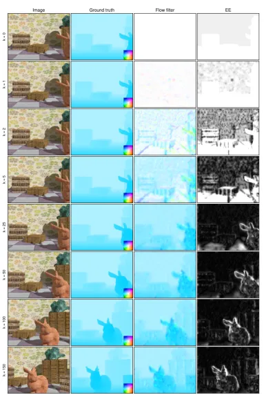
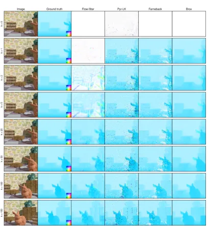
2.6 Experimental Results . . . 31
2.6.1 Ground truth optical flow dataset . . . 31
2.6.2 Error metrics . . . 32
2.6.3 Evaluation on the Bunny sequence . . . 32
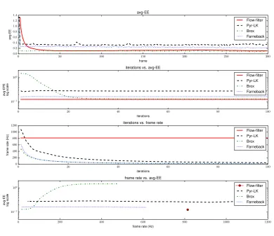
2.6.3.1 Runtime vs. error performance . . . 33
2.6.4 Evaluation on the Middlebury test dataset . . . 34
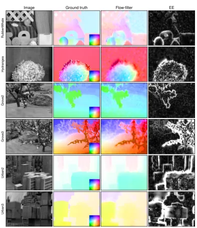
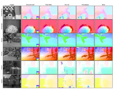
2.6.5 Evaluation on real-life high-speed video . . . 36
2.6.6 Runtime performance on embedded GPU hardware . . . 40
2.7 Summary . . . 41
3 Spherepix: a Data Structure for Spherical Image Processing 45
3.1 Outline . . . 47
3.2 Background . . . 47
3.2.1 Sphere pixelations . . . 47
3.2.2 Computer vision algorithms on the sphere . . . 48
3.3 Geometry . . . 50
3.3.1 Orthonormal coordinate system . . . 53
3.4 The Spherepix Data Structure . . . 54
3.4.1 Pixelation properties . . . 55
3.4.2 Coordinate interpolation . . . 56
3.5 Low-level Image Processing Operations . . . 58
3.5.1 Camera mapping . . . 58
3.5.2 Low-level image processing routines . . . 59
3.5.2.1 Gaussian filtering . . . 59
3.5.2.2 Image gradient . . . 62
3.5.3 Patch reconciliation . . . 62
3.6 Applications . . . 63
3.6.1 SIFT feature point extraction . . . 63
3.6.2 Dense optical flow computation . . . 67
3.7 Summary . . . 69
4 Real-time Structure Flow 71 4.1 Outline . . . 74
4.2 Background . . . 74
4.2.1 Kinematics . . . 74
4.2.2 Scene and optical flow on the image plane . . . 75
4.2.3 Estimation of scene flow . . . 76
4.2.4 Real-time algorithms . . . 77
4.3 Optical, Scene and Structure Flow on the Sphere . . . 77
4.4 Evolution equations . . . 81
4.4.0.1 Image brightness . . . 81
4.4.0.2 Structure flow . . . 82
4.4.0.3 Depth and inverse depth . . . 82
4.5 Filter Algorithm . . . 83
4.5.1 Brightness parameter extraction . . . 84
4.5.2 Inverse depth parameter extraction . . . 85
4.5.3 State prediction (k→k+) . . . 86
4.5.4 State update (k+→k+ 1) . . . 87
4.6 Numerical prediction . . . 90
4.7 Experimental Results . . . 92
4.7.1 Ground truth evaluation . . . 92
4.7.2 Evaluation on real-life data . . . 96
Contents xiii
5 Conclusions 99
5.1 Achievements . . . 99 5.2 Future Work . . . 100
A Ground Truth Optical Flow for a Perspective camera 105
B Numeric Solution to Spherepix Spring Regularization 107
List of Figures
1.1 Scene, optical and structure flow. . . 2
2.1 300 Hz incremental computation of optical flow. . . 9
2.2 Top level optical flow filter architecture. . . 18
2.3 Lower levels optical flow filter architecture. . . 18
2.4 Brightness model parameters computation. . . 19
2.5 Upwind direction with respect to optical flow. . . 25
2.6 One-dimensional optical flow propagation. . . 28
2.7 Numerical propagation of optical flow. . . 29
2.8 Numerical propagation of image field by the optical flow. . . 30
2.9 Panoramic view of Bunny 3D environment. . . 32
2.10 Flow-filter algorithm results on the Bunny sequence. . . 35
2.11 Estimated optical flow on the Bunny sequence. . . 36
2.12 Trade-off between accuracy and runtime performance in the Bunny sequence. . 37
2.13 Results in the interpolated Middlebury test dataset. . . 38
2.14 Evaluated algorithms in the Middlebury test dataset. . . 39
2.15 Youtube video layout. . . 41
2.16 ANU campus drive sequence. . . 43
2.17 ANU campus drive sequence: flow-filter and PyrLK comparison. . . 44
3.1 Catadioptric image mapped onto Spherepix patches. . . 45
3.2 HEALPix pixelation. . . 49
3.3 Cubed-sphere pixelation. . . 49
3.4 Yin-Yang pixelation. . . 50
3.5 Projection-retraction classes on the sphere. . . 51
3.6 Orthonormal coordinates in tangent spaceTη0S2. . . 53
3.7 Spherepix mass-spring system. . . 55
3.8 Patch subdivision modes. . . 55
3.9 Spherepix regularization measurements. . . 56
3.10 Orthonormal grid coordinates in tangent spaceTηijS 2. . . . 57
3.11 Spherepix patch interpolation belt. . . 57
3.12 Camera mapping onto the sphere. . . 60
3.13 Omnidirectional image mapping onto Spherepix. . . 61
3.14 Image gradient computation. . . 63
3.15 Panoramic rendering of Spherepix image. . . 64
3.16 Synthetic ommnidirectional images. . . 65
3.17 Recall vs rotation angle and Recall vs. 1 - Precision curves. . . 65
3.18 spixSIFT feature point extraction. . . 66
3.19 Dense optical flow computation. . . 68
3.20 Panoramic view of optical flow in tangent space coordinates. . . 69
4.1 Structure flow field. . . 71
4.2 Scene, optical and structure flow. . . 73
4.3 Kinematics of pointxexpressed in the camera body fixed frame. . . 74
4.4 Scene, structure and optical flow for a spherical camera. . . 77
4.5 Scene, structure and optical flow fields for a forward moving camera. . . 80
4.6 Structure flow pyramidal filter architecture. . . 84
4.7 Brightness parameters extraction. . . 85
4.8 Structure flow PDE source terms. . . 88
4.9 Numerical propagation of structure flow, image brightness and inverse depth. . 93
4.10 Urban Canyon dataset. . . 94
4.11 Results on the Urban Canyon dataset. . . 95
4.12 Error metrics for the Urban Canyon dataset. . . 96
List of Tables
2.1 Real-time optical flow methods. . . 15
2.2 Finite difference operators in thexandyaxes for a scalar fieldc. . . 25
2.3 Shift operators. . . 26
2.4 Parameters of evaluated algorithms in the Bunny sequence. . . 33
2.5 Results summary for the Bunny sequence. . . 34
2.6 Parameters of evaluated algorithms in the Middlebury test sequences. . . 37
2.7 Average Endpoint Error results in the Middlebury test dataset. . . 39
2.8 Average Angular Error results in the Middlebury test dataset. . . 40
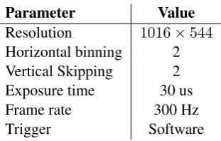
2.9 Basler USB3 camera parameters. . . 40
2.10 Flow-filter parameters for real-life high-speed video sequences. . . 41
2.11 Flow-filter Youtube videos. . . 41
2.12 Runtime performance on Nvidia Tegra K1 SoC and desktop GTX 780 GPU. . . 42
4.1 Difference operators in beta coordinates. . . 86
4.2 Runtime performance with one pyramid level at512×512resolution. . . 96
4.3 Runtime performance with two pyramid level at512×512resolution. . . 96
4.4 Runtime performance with two pyramid level at1024×1024resolution. . . 97
Chapter 1
Introduction
Genius is one percent inspiration and ninety-nine percent perspiration.
Thomas Alva Edison
Vision offers rich sensor information to robotic vehicles interacting in complex dynamic environments. As robots are increasingly deployed in unconstrained dynamic environments, the requirements of the visual system become more demanding in terms of accuracy and re-sponse time. Thanks to the expansion of the mobile phone industry, image sensors and embed-ded processors have experienced an increase in compute performance as well as a reduction in price, making the use of such technologies cost effective within the robotics industry. However, the extraction of meaningful information from a vision sensor is a complicated and computa-tionally intensive task.
The focus of this thesis is on the design and implementation of dense real-timevisual flow
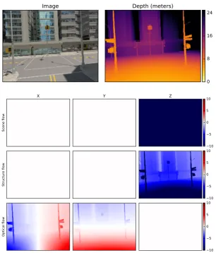
algorithms. A visual flow field is a vector field on the camera’s image surface that provides motion information for each pixel in the image. There are at least three types of visual flows, illustrated in Figure 1.1a, that can be extracted from image sequences: scene flow,optical flow
and the novelstructure flowthat I introduce in Chapter 4. Thescene flow, so called by Vedula et al. [1999], is the three-dimensional motion field of points in the world relative to the camera. That is, the Euclidean 3D velocity between the closest object in the scene at a given pixel location and the robot’s camera.Optical flowis the projection of the scene flow onto the image plane of the camera. It describes the velocity of each pixel in the image plane induced by the motion of the robot and the environment Barron [1994]. Structure flow, introduced in this thesis Adarve and Mahony [2016b], sits in between scene and optical flow. Mathematically, structure flow is the three-dimensional scene flow scaled by the inverse depth at each pixel in the image. Intuitively, it is the complete velocity field associated with image motion, including both optical flow and scale-change or apparent divergence of the image. Analogously to optic flow, structure flow provides a robotic vehicle with perception of the motion of the environment as seen by the camera. However, structure flow encodes the full 3D image motion of the scene whereas optic flow only encodes the tangential image motion.
From an algorithm complexity perspective, optical flow is the easiest to compute from image data among the three types of visual flow. Estimation of dense optical flow can be seen as a dense registration of two images separated in time Lucas and Kanade [1981]. For
(a) Scenev∈R3, structurew∈R3and optical flowΦ∈R2vectors for a pointxin the scene. Pointx moves with a relative velocity (scene flow)vwith respect to the camera body fixed frame, and projects to pixelpon the image plane. The optical flowΦatpis a two-dimensional projection of scene flow on the image plane. The structure flow vectorwis the scaling of the scene flow by the inverse of the distanceλtox.
Depth (meters)
0 8 16 24
Image
Optical flow
10 5 0 5 10 Y
Scene flow
X Z
10 5 0 5 10
10 5 0 5 10
Structure flow
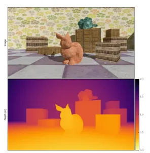
[image:20.595.124.431.336.695.2](b) Scene, structure and optical flow fields for a perspective camera mounted on a forward moving vehicle at 10m/s. The simulated perspective camera runs at 100 Hz.
3
each pixel in the first image, a displacement vector is computed such that the brightness value in the second image matches. Consequently, computation of optical flow is purely a data matching process, and it does not depend directly on the underlying scene or camera geometry. Algorithms for estimating optical flow can be counted by the hundreds and they have been summarized over the last two decades in the survey papers of Barron [1994] and Baker et al. [2011]. Optical flow has been widely used in robotic systems. Application examples include: visual servoing Hamel and Mahony [2002], vehicle landing on a moving platform Herisse et al. [2012], height regulation Ruffier and Franceschini [2005] and obstacle avoidance Srinivasan [2011a].
Computation of Scene flow is less studied than optical flow. State of the art algorithms using two-pair stereo-images can be found in the Kitti scene flow dataset of Menze and Geiger [2015]. Other approaches such as those using RGB-D sensors (e.g., the Microsoft Kinect) have also been studied Hadfield and Bowden [2011], Herbst et al. [2013]. Real-time scene flow algorithms are relatively slow compared to optical flow, running between 20-30 Hz Rabe et al. [2010], Wedel et al. [2011]. Runtime performance of modern two-pair stereo based approaches are reported in the Kitti scene flow dataset1.
Figure 1.1b illustrates the scene, structure and optical fields for a vehicle moving at 10m/s in collision course with a building located approximately at 15 meters. The image and depth map are from the visual odometry dataset of Zhang et al. [2016]. The simulated perspective camera (with the Z axis matching the camera focal axis) runs at 100 Hz and all flow fields are expressed in pixel units. Since the simulated scene is static, the calculated scene flow is equal for all pixels in the image and is equal to the negative of the camera velocity. As the vehicle moves along the focal axis of the camera, the xy component of the scene flow are zero. Scaling the scene flow by the inverse of the depth field, we obtain the structure flow field. The structure flow distinguishes between objects close to or far away from the camera since the relative angular divergence of closer objects is larger. That is, they are growing in the image more quickly than distant objects. Last row of Figure 1.1b is the optical flow field on the image plane of the camera. Since optical flow is the projection of the scene flow onto the image plane, thez component of the optical flow is zero. That is, no motion along the focal axis of the camera. In fact, the optical flow is a divergent vector field with the focus of expansion located in the center of the image; the direction of motion. Notice that, although the vehicle is moving quickly, the optical flow in the central region of the image is small, and it is difficult to evaluate the time to contact before the vehicle collides with the building.
Current algorithms developed within the Computer Vision community aim at improving the accuracy of the estimated optical flow fields. This trend can be observed in the latest re-sults of standard optical flow benchmark datasets Baker et al. [2011]; Butler et al. [2012]; Geiger et al. [2013]. At the same time, the complexity of the top performing algorithms has increased and thus their computational demands, as reported in the benchmarks. While these algorithms can be used in applications where runtime performance is not a critical constraint, their application on real-time vision pipelines, as those required by robotic platforms, is ques-tionable.
An underlying requirement of any visual flow algorithm in a robotic system is the capability
to perform computations in real-time. If the output of the algorithm is to be used as direct sensor feedback by the controller, ‘real-time’ means at least as fast as the frequency at which the control system works and preferably 5-10 times faster. For a typical aerial vehicle, this means the visual system needs to operate at frequencies in the order of 200-500 Hz Bangura et al. [2015]. Moreover, due to power and weight limitations of the vehicle, computations have to be carried out on embedded compute platforms with limited computational resources. As a consequence, typical robotic systems use rather simple algorithms, such as Srinivasan [1994] and Bouguet [2001] for computing optical flow, compared to the state of the art in Computer Vision.
Algorithms such as those mentioned above were designed using a two-frame approach in which the algorithm gives a dense output for each pair of frames. While this is the typical approach for computing optical flow, it does not match the intrinsic properties of a robotic vision system. Those are:
• High-speed video capture: Robotic vision systems can take advantage of high-speed image sensors to sample the evolution of the environment at high frame rates. As the environment is sampled faster, the relative change between any two consecutive frames gets smaller. In the limit, with a camera working at multiple hundreds of Hertz, the difference between any two images would be expected to be at the sub-pixel level.
• Additional sensor modalities: A typical robotic vehicle contains several sensors, such as inertial measurement units and laser scanners, that can be integrated into the visual system. Information provided by these sensors can be fused within the vision algorithms to create a robust and coherent representation of the environment surrounding the robot.
A key challenge of using high-speed image sensors is processing the stream of data in real-time. As an example, the high-speed camera used in the experiments of this thesis provides
1016×544images with 256 brightness levels per pixel at 300 Hz. This is equivalent to 158 Megabytes of image data to be processed every second. This resolution and frame rate places a heavy load on the available computational resources such as USB3 and RAM bandwidth as well as the compute resources of typical GPU hardware.
Considering the properties mentioned above, I proposed the termRobotic Embedded Vision
(REV) system to describe an electronic system and a set of algorithms to offer visual sensing capabilities to a robotic vehicle. A REV device contains vision sensors connected directly to processing elements (CPU, GPU or FPGA) as well as extra sensors, such as IMU or GPS, to provide additional information to the algorithms. Vision algorithms are executed inside the REV device, reducing the latency between image acquisition and processing. The output of the vision algorithms (optical flow, feature points, etc) is then used according to the robot’s current task, and only information required to perform such task is transmitted to the robot CPU. An application example is the transmission of velocity commands for an aerial vehicle according to the perceived optical flow. Notice that only the result of the algorithm is transmitted out of the device. This can potentially reduce the required bandwidth of the communication channel between the REV system and the robot CPU.
§1.1 Contributions 5
into consideration the properties of a robotic vision system mentioned above to create real-time algorithm formulations and implementations. Both optical and structure flow algorithms follow a filtering approach for estimating the underlying visual flow. The filters follow the standard prediction-update approach to incrementally build a dense estimate of flow using new sensor measurements and predictions made using the old state.
There are two advantages of using a filtering approach. First, thanks to the incremental nature of the algorithm, the output of the algorithm is temporally consistent. The state estimate at time k+ 1 is equal to the old estimate at time k plus some innovation considering new measurements. Second, a filtering approach can reduce the amount of computations required at each time step. Instead of computing highly accurate and dense flow fields using two images, that is, following the standard approach, an incremental algorithm does partial computations at every time step and adds new information to the state. Dense and accurate state estimates are reached over time.
An important contribution of this thesis is the use of partial differential equations (PDE) to model the spatio-temporal evolution of the optical and structure flow fields on the image surface. Efficient numerical methods that match the massive parallel compute power of GPU and FPGA platforms are developed to solve these PDEs.
For each visual flow algorithm, experimental validation is provided using both ground-truth data simulating a high-speed camera mounted on a mobile vehicle. Additionally, results on real-life videos captured are provided to validate the algorithms; for optical flow, a 300 Hz high-speed monocular camera is used, while a 60 Hz stereo camera array is used to test the structure flow algorithm. All the algorithms were implemented and tested on a Nvidia GTX 780 Desktop GPU card and partially tested on a embedded Nvidia Tegra K1 System on Chip.
1.1
Contributions
The following are the contribution of this thesis towards the design and development of real-time visual flow algorithms for robotic applications.
• Optical flow filter: A filtering algorithm for the computation of dense optical flow in real-time is proposed. The algorithm uses a predictor-update approach for the incre-mental estimation of optical flow. The prediction part is the first one to introduce the PDE approach for modeling the spatio-temporal evolution of the flow field on the image plane. A GPU implementation of the algorithm is developed and it is currently available as an open-source software. The algorithm can run at frame rates of more than 300 Hz on commodity Desktop GPU hardware.
• Spherepix data structure for spherical image processing: The Spherepix data struc-ture is a discretization of the unit-sphere on which low-level image operations such as Gaussian filtering and gradient computation can be efficiently implemented. Spherepix provides the numerical layer on which the structure flow filter algorithm is implemented.
1.2
Publications
Published
1. Adarve, JD., Li, W., Mahony, R. and Austin, D.,Towards an Efficient and Robust Op-tic Flow Algorithm for RoboOp-tic Applications, Australasian Conference on Robotics and Automation. 1-9, 2012.
2. Adarve, JD., Austin, D. and Mahony, R.,A Filtering Approach for Computation of Real-Time Dense Optical-flow for Robotic Applications, Australasian Conference on Robotics and Automation. 1-10, 2014.
3. Adarve, JD. and Mahony, R., A Filter Formulation for Computing Real Time Optical Flow, IEEE Robotics and Automation Letters, Vol. 1, 1192-1199, 2016.
4. Adarve, JD. and Mahony, R.,Spherepix: a Data Structure for Spherical Image Process-ing, IEEE Robotics and Automation Letters, Vol. 2, 483-490, 2016.
Under review
1. Adarve, JD. and Mahony, R.,Real-time Structure Flow, IEEE Transactions on Robotics.
1.3
Software Packages
1. Optical-flow-filter: https://github.com/jadarve/optical-flow-filter. Implementation of the optical flow filtering algorithm in CUDA. The repository provides demo appli-cations to run the algorithm from images captured from a webcam (OpenCV based) and from a high-speed Basler USB3 camera.
2. Spherepix: https://github.com/jadarve/spherepix. Implementation of the Spherepix data structure for processing of spherical images.
3. Structure-flow-filter: (To be released). Implementation of the structure flow filtering algorithm in CUDA.
1.4
Thesis Outline
§1.4 Thesis Outline 7
• Chapter 2presents the filtering approach for the computation of dense optical flow in real time. It provides a review of optical flow algorithms, in particular real-time methods used in robotic applications. The results section provides ground truth validation of the algorithm as well as qualitative comparison on high-speed 300 Hz real-life video taken in a driving scenario.
• Chapter 3describes theSpherepixdata structure for efficient implementation of com-puter vision routines on spherical images. The literature review focuses on general-purpose computer data structures for the discretization of the sphere, as well as the state of the art on computer vision algorithms on spherical images. The mathematical con-cepts in this chapter are fundamental to understand the numerical implementation of the Structure Flow algorithm in Chapter 4.
• Chapter 4develops theStructure Flowfield. The literature cited in this chapter focuses on the estimation of 3D motion fields from image or depth measurements (scene flow). This chapter develops the partial differential equations modeling the spatio-temporal evolution of the structure flow field on spherical camera geometry. Additionally, a filter-ing algorithm for the estimation of structure flow in real time is formulated and evaluated on ground-truth and real-life video sequences.
Chapter 2
A Filter Formulation for Computing
Real-time Optical Flow
Keep It Simple - Run It Fast
Juan Adarve
Flo
w
(color
encoded)
10.0 ms
Input
image
0.0 ms 30.0 ms 300.0 ms
Flo
w
magnitude
(pix.)
0.0 0.5 1.0 1.5 2.0
Figure 2.1: 300 Hz incremental computation of optical flow. Images captured with a high-speed camera are used to extract the underlying optical flow of the scene.
Optical flow is the two-dimensional vector field describing the motion of pixels in the im-age plane due to the motion of the environment and the camera. Optical flow offers important visual cues to a robotic vehicle moving in a dynamic environment. Applications such as visual servoing Hamel and Mahony [2002], vehicle landing Herisse et al. [2012], height regulation Ruffier and Franceschini [2005] and obstacle avoidance Srinivasan [2011a] use the estimated optical flow computed by the onboard vision system of the robot.
In a robotics context, an important requirement of any optical flow algorithm is its capa-bility to run at real-time frequencies. In practice, this means that the vision processing system should run at the same frequency, or preferably faster, than the vehicle controller. For a typi-cal high-performance autonomous vehicle, this translates to frame rates in the order of 200Hz Bangura et al. [2015]. Furthermore, typical robotic platforms have weight limitations that
strain the amount of compute hardware they can carry. For example, small aerial vehicles use similar embedded System on Chip (SoC) as those found in modern smart-phones. These chips are equipped with multi-core processing units as well as mobile Graphics Processing Units (GPU).
Real-time computation and embedded hardware constraints requires a different approach to compute optical flow from the state of the art algorithms documented in the well known benchmarks such as Baker et al. [2011]; Butler et al. [2012]; Geiger et al. [2013]. Typical algorithms from the Computer Vision community use two frames to estimate dense optical flow between the two images Baker et al. [2011]. In order to achieve highly accurate results, modern algorithms use sophisticated mathematical models to extract the optical flow from two frames. Typically, the most accurate algorithms are also the more computationally expensive, as it can be verified in the runtime reported in benchmark datasets cited above.
Recall the properties of a Robotic Embedded Vision system (REV) described in chapter 1, in particular thehigh-speed video samplingof the environment to capture the dynamics of objects in the world at high frequencies. This chapter proposes a new optical flow algorithm capable of running at frequencies as high as 800Hz at640×480on a Desktop computer and near 100 Hz on embedded GPU SoC at320×240pixel resolution.
The proposed algorithm follows a prediction-update filtering approach, where an internal optical flow state is incrementally built and updated using the stream of image data from the camera. An important component of the algorithms is the prediction stage, which is modeled as a system of partial differential equations to integrate forward in time the current estimation of image brightness and optical flow to create predictions for future time. Numerical solution to these equations is implemented using an efficient finite difference method based on upwind differences Thomas [1995]. This numerical method can be efficiently implemented on both GPU and FPGA hardware.
2.1
Outline
This chapter is divided as follows. Section 2.2 provides the relevant literature on optical flow and real-time algorithms. Section 2.3 develops the idea of incremental computation of optical flow. Section 2.4 explains the details of the filtering algorithm. Section 2.5 develops the numerical implementation of the propagation stage using finite difference methods. Section 2.6 provides the experimental results on both synthetic and real-life high-speed image sequences. Finally, the chapter is closed in Section 2.7 with some summary comments.
2.2
Background
Optical flow is the two-dimensional vector field describing the velocity of each pixel in a sequence of images. The computation of optical flow is one of the fundamental problems in computer vision and can be traced back beyond the seminal works of Lucas and Kanade [1981] and Horn and Schunck [1981].
§2.2 Background 11
used as: differential techniques, region based methods, energy based methods and phase based methods. From these, differential and region based methods are of interest in the context of this thesis.
• Differential techniques:Differential methods use spatio-temporal models of the image brightness to recover the underlying optical flow from a sequence of images. These methods are based on the brightness conservation assumption that states that the total amount of brightness in the image is conserved over time. Intuitively, this means that any change in the brightness value of a given pixel is due to the change in position of the object in the scene in that pixel direction.
Early works in optical flow such as those of Lucas and Kanade [1981] and Horn and Schunck [1981] are differential methods. These two algorithms marked a distinction be-tween local based (Lucas-Kanade) and global based methods (Horn-Schunck) for com-puting flow. Local based methods use a small support window around each pixel in the image to estimate optical flow, while global based methods impose a global constraint over the optical flow field to improve the quality of the estimation. In general, local based methods are faster than global based ones. A detailed explanation of these algorithms is provided in Section 2.2.2.
Modern differential algorithms Brox et al. [2004]; Bruhn et al. [2005]; Werlberger [2012] utilize the same differential principles together with robust optimization frameworks to create highly accurate flow estimates. In particular, global based methods often use the L1 norm instead of the L2 (as in Horn and Schunck) to be more robust to outliers in the estimation process.
• Region based algorithms:Region based methods to compute optical flow can be thought as a search process to find a patch of texture in the second image that matches a reference patch in the first. A key difference of this approach compared to differential techniques is that it does not make the assumption of the image brightness to be differentiable.
Early works such as that of Anandan [1989] uses thesum of square differences(SSD) to match texture patches within in a search region for each pixel. In order to support large pixel displacements, the algorithm is formulated in a pyramidal structure where coarse estimates of flow are computed on low resolution images and then are refined using higher resolution data. Srinivasan image interpolation algorithm follows a similar approach to find optical flow Srinivasan [1994], and has been used in real-life robotic systems Srinivasan [2011a].
Modern algorithms such as SimpleFlow byet. al.Tao et al. [2012], PatchMatch by Bao et al. [2014], Piecewise Parametric Flow by Yang and Li [2015] and many others have proven the effectiveness of region based methods on public benchmarks.
More recent algorithms are listed on different benchmark datasets. The most relevant are: the Middlebury flow dataset by Baker et al. [2011]1, the Kitti dataset by Geiger et al. [2013]2 and the Sintel dataset by Butler et al. [2012]3. Each of these datasets provide both test and
1http://vision.middlebury.edu/flow/
2http://www.cvlibs.net/datasets/kitti/eval_flow.php
evaluation sequences to evaluate optical flow algorithms. The image sequences can be both real-life images, for which the ground truth is computed using fluorescent markers as in the Middlebury dataset or using odometry and laser measurements as in the Kitti dataset. The Sintel dataset is a purely synthetic dataset based on the Sintel open-source movie4 created in Blender5. Ground truth optical flow can be extracted directly from the scene geometry (depth map) and the motion of objects relative to the camera.
Additionally, the survey article of Sun et al. [2014] offers a review of most recent al-gorithms together with a quantitative analysis of different optimization frameworks used to estimate optical flow. Also, the survey article of Chao et al. [2014] offers a list of optical flow algorithms currently used in robotic applications.
Optical flow algorithms are too numerous to create an exhaustive classification and review. Instead, the review provided in this chapter is focused on algorithms that have proven to work at real-time frequencies, thus making them effective for real-life robotic applications. In par-ticular, differential optical flow algorithms are reviewed in detail, as such algorithm are closer to the mathematical formulation used in this chapter. Additionally, bioinspired algorithms as well as methods using alternative camera technologies such as Dynamic Vision Systems are included in this review.
2.2.1 Differential methods for optical flow computation
The most common algorithms to compute optical flow are the differential methods. These methods model the temporal change of intensity due to the underlying optical flow present in the image sequence. The approach is based on the well known brightness conservation equationthat is the starting point of all differential methods Barron [1994].
Let Y(p, t) : R2 ×R → R denote the image brightness at pixel position p ∈ R2 and timet∈R. The common assumption about image brightness is that the objects composing the scene are made of Lambertian materials. That is, the light scattered by the material is invariant to the viewer’s view angle. Given this assumption, it is possible to say that the value of image brightness is constant over time. In other words, the total rate of change of image brightness over time is zero. Mathematically, one has
dY
dt = 0 (2.1)
Since brightness is a function of independent variablespandt, one can decompose Equa-tion (2.1) in terms of its partial derivatives as
dY
dt = ∂Y ∂p
dp dt +
∂Y
∂t = 0 (2.2)
where ∂Y∂p ∈ R2 is the image gradient vector and ddpt ∈ R2 is the relative change in pixel position, that is, the optical flow atp. Equation (2.2) is thebrightness conservation equation
modeling the relationship between temporal brightness change and optical flow, and is the common starting point of all differential techniques.
4https://durian.blender.org/
§2.2 Background 13
Equation (2.2) imposes only one constraint to the two-dimensional optical flow vector ddpt. That is, only the component of ddpt parallel to the image gradient ∂Y∂p is relevant to (2.2). This is known as theaperture problemin the literature. Algorithms need to use some form of data integration or regularization to recover the full two-degrees of optical flow.
In differential methods, there are two families of algorithms to find the optical flow from a sequence of images. The first family, local-based methods, consists in algorithms that use a local support window around each image pixel to find the underlying optical flow. The second family,global-based methods, impose global constraints over the whole image that the resulting optical flow field must satisfy.
Local-based methods use a finite support window around each image pixel to find optical flow. Within this window, flow is assumed to be constant and all image data within the window is used to recover one single flow vector. The most popular algorithm of this family was proposed by Lucas and Kanade [1981]. LetΩpdenote a support window around pixelp. The
basic formulation of Lucas-Kanade method is to minimize cost function
εp,Φ =
X
q∈Ωp
k∂pYqΦ+∂tYqk2 (2.3)
for the unknown optical flowΦ:= ddpt atp. Here∂pYqdenotes the image gradient vector at
pixelqand∂tYqis the image temporal derivative atq.
A popular implementation of Lucas-Kanade method is the one developed by Bouguet [2001] and available in OpenCV6. To support large optical flow fields, this implementation uses a pyramidal approach to subdivide the problem in different image scales. At coarse scale, the algorithm computes a coarse estimation of flow from the low resolution data. This coarse estimate is refined using higher resolution data from the next scale level, until the original resolution level is reached.
Local based methods, in general, are subject to noise in the data within the support window. In regions of the image where there is no gradient information, that is, in textureless regions of the image, it is not possible to recover optical flow. Moreover, the estimated optical flow suffers from the aperture problem, where only the flow in the direction of the image gradient can be computed.
Global-based methodsimpose a prior constraint over the optical flow at each pixel. Typi-cally, this prior has the form of a smoothness constraint where the optical flow field is assumed to be smooth across the image. One example of global based methods is the seminal work by Horn and Schunck [1981]. In their work, the authors formulate the optical flow problem as a variational problem where the brightness conservation equation is complemented with a flow smoothness term to regularize the computation of flow in image regions with poor texture data. The goal is to minimize cost functional in Equation (2.4) with respect toΦ.
ε2=
Z Z
k∂pYΦ+∂tYk2+α2(∂xφx)2+ (∂yφx)2+ (∂xφy)2+ (∂yφy)2dxdy (2.4)
Equation (2.4) can be solved using calculus of variations, expressing the integral in terms of its underlying Euler-Lagrange system of partial differential equations. The resulting system
couples the solution of each pixel and its neighbors, and requires an iterative method to find the solution (for example, Gauss-Jordan method).
The key advantage of global-based methods over local-based ones is that estimations at each pixel are well defined thanks to the smoothness term. In regions of the image where image gradient information is poor, the smoothness term in Equation (2.4) dominates over the image term. Consequently, the flow in those regions will be filled with flow coming from regions with high texture content such as image edges.
The work of Horn and Schunck opened a new research field in computer vision for the computation of optical flow using variational methods. One of such algorithms is proposed by Broxet. al. Brox et al. [2004] which is used as reference in the experimental evaluation in Section 2.6. Global-based methods typically outperform local-based methods in terms of accuracy in benchmarks such as Middlebury, Kitti and Sintel. However, local based methods perform better in terms of runtime, as it will be illustrated in the next section.
2.2.2 Real-time algorithms and systems
This section describes real-time optical flow algorithms and systems. This separation from mainstream optical flow algorithms is important in a robotics context, where algorithm’s run-time is as important as its accuracy.
In general, real-time flow algorithms are local-based methods. Many of these methods are some form of Lucas-Kanade method Lucas and Kanade [1981], region based method, like Srinivasan [1994], or neuromorphic approaches Mueggler et al. [2014]. Image data is con-strained to a local support window around each pixel. Moreover, the algorithms are designed such that the flow estimation is independent for each pixel, thus allowing one to perform com-putations in parallel for each all pixels. This pixel independence allows algorithm implemen-tation on multi-core processors or Graphic Processing Units (GPU). Moreover, it is possible to create digital circuit pipelines to compute optical flow directly in silicon. Prototypes of these pipelines can be deployed and tested on Field Programmable Gate Arrays (FPGA) chips.
Table 2.1 lists relevant real-time dense optical flow methods found in the literature. For each algorithm, its resolution (pixels), working framerate (Hz) and throughput (Mpix/s) is reported. The throughput is computed as
Tput= resolution·framerate
106 (2.5)
Typically, real-time optical flow algorithms are implemented on GPU hardware to take ad-vantage of the parallel compute power to perform per-pixel operations simultaneously. Bouguet [2001] created a pyramidal implementation of the Lucas-Kanade optical flow method freely available in OpenCV both in CPU and GPU versions. The GPU version is used in Section 2.6 to compare both the accuracy and performance of the optical flow filter algorithm. The eFOLKI algorithm of Plyer et al. [2014] is an implementation of the Lucas-Kanade method that increases the robustness of the algorithm by applying a Rank-n transform Zabih and Woodfill [1994] before minimizing a SSD cost function to find the optical flow.
§2.2 Background 15
external memory bank. The systems by Plett et al. [2012] and Zhang et al. [2008] are inspired by the visual cortex of insects to compute local motion descriptors.
Resolution Framerate (Hz) Tput. (Mpix/s) Hardware
Adarve and Mahony [2016a] 640×480 814 250.06 GPU
Derome et al. [2016] 1242×375 10 4.65 GPU
Kroeger et al. [2016] 128×54 600 4.14 CPU
Plyer et al. [2014] 640×480 166 60 GPU
Barranco et al. [2013] 640×480 31 9.52 FPGA
Plett et al. [2012] 240×240 350 20.16 FPGA
Anguita et al. [2009] 1280×1016 68.8 89.47 CPU
Zhang et al. [2008] 256×256 320 20.97 FPGA
Farnebäck [2003] 640×480 27 8.29 GPU
Bouguet [2001] 640×480 33 10.13 GPU
Table 2.1: Real-time optical flow methods. Image resolutions and framerate were copied from the original papers.
2.2.3 Neuromorphic approaches
There are alternative image sensors and algorithms inspired by nature from which it is possible to extract optical flow. These technologies and algorithms are of particular importance to robotics as they offer fast visual feedback to robotic vehicles.
One of such approaches comes from understanding the visual system of insects. Insects such as flies and bees have compound eyes made of a grid of light sensors known as the ommatidia. Each ommatidium captures a narrow field of view of the scene and is connected to the visual cortex of the insect. The reader is encouraged to read the review paper by Borst on the structure of insect’s eye Borst [2009]. It is possible to model the correlation between neighboring ommatidium to extract motion information. This correlation model is known as the Reichardt motion detector Reichardt [1987]. Systems such as those by Zhang et al. [2008] and Plett et al. [2012] have demonstrated the effectiveness of this motion detector in real-life systems.
The work by Srinivasan [2011a,b] offers an insight on how the motor control part of the insects’ neural cortex connects to the visual system. In his experiments, he has demonstrated how honeybees use optical flow for tasks such as navigation, obstacle avoidance and landing. The understanding of insect vision has brought insight to robotics to solve the same tasks on flying vehicles. Such is the case of the works by Ruffier and Franceschini on optical flow regulation Ruffier and Franceschini [2005], the work of Mafricaet. al.on velocity and steering angle control of a car vehicle Mafrica et al. [2016] and the work by Herisse et al. [2012] on landing and take-off of an aerial vehicle from a moving platform using optical flow.
image frames. An event is triggered by a temporal change in pixel brightness. Current hard-ware7transmits event location, timestamp and polarity (plus or minus) asynchronously. Conse-quently, the bandwidth required between camera and processing units is significantly reduced, as the camera only transmits the difference between two images. Applications of this technol-ogy are emerging: Benosman et al. [2012, 2014] extract optical flow from the event stream using a differential framework similar to that used on standard gray-scale images. Mueggler et al. [2014] use the stream of events to track the 6-DOF pose of an aerial vehicle using the on-board vehicle’s CPU.
2.3
Incremental Computation of Optical Flow
The main concept in the development of the proposed real-time optical flow algorithm is that of incrementally building a dense flow estimate over time. In this approach, one has an internal optical flow state that is constantly refined using new image measurements from the camera. Instead of computing dense flow fields from two images, as typical computer vision algorithms do, an incremental approach will exploit the large availability of data one has in a real-life robotic vision system to constantly estimate optical flow.
This incremental approach has two advantages over standard algorithms. First, the opti-cal flow field is temporally smooth. Thanks to the incremental nature of the algorithm, the temporal evolution of the estimated flow field will show a smooth transition between two con-secutive image frames. Second, there are computational efficiencies in this approach. Instead of using a complex algorithm to compute dense optical flow fields from two images, one can design a simpler flow update algorithm considering new image data and the current flow state estimation.
Intrinsic to the incremental approach to compute optical flow, is the concept of temporal evolution of the flow field. At each time step, that is, when a new image arrives, one needs to propagate forward in time the old flow state to align it to current time. Once the prediction is completed, both the flow state and the measurements are temporally aligned, and a new estimate of optical flow can be created using both pieces of information.
This process matches a filter architecture consisting of update and prediction stages. To the best of the author’s knowledge, this architecture for computing optical flow was first described in the PhD dissertation of Black [1992]. In his work, Black uses robust statistic methods in the update stage to refine the predicted optical flow from previous time step. The prediction is formulated as the warping of the optical flow field forward in time. This warping can be implemented by adding the optical flow field to each pixel coordinate and then performing a re-sampling of the resulting image.
The proposed algorithm in this chapter follows the same general update-prediction archi-tecture. However, a key novelty is the formulation of the prediction stage as system of partial differential equations modeling the transport of optical flow, and any associated field, by the optical flow. The prediction stage is implemented by numerically solving these transport PDEs using a finite difference solver. In contrast to image warping, the finite difference solver does work on a fixed grid of points and hence, it does not require a re-sampling post-processing
§2.4 Filter Architecture 17
stage.
As it will be shown throughout the chapter, this filter formulation leads to regular compu-tations that can be realized in both GPU and FPGA hardware, and can run at the frequencies required by a robotic vision system.
2.4
Filter Architecture
The optical flow filter algorithm is constructed as a pyramid of filter loops. Let H be the number of levels of the pyramidal structure, andh = 1, . . . Hthe level index. The filter state at time indexkis the pyramid of vector fieldsXk =
Φ
H k,H-1∆Φk, . . . ,1∆Φk . The state at
levelHis the optical flow fieldHΦk(p) :
R2 →R2estimated using low resolution image data. For levelsh =H−1, . . . ,1the state is defined as the vector field h∆Φk(p) :
R2 → R2that refines the optical flow from the level immediately above using higher resolution data available at levelh.
The reconstruction of optical flow at lower levels is achieved by iterating Equation (2.6) forh=H−1, . . . ,1
Φ
h k
= 2h+1:hΦk
+h∆Φk
(2.6)
where h+1:hΦk denotes the upsampling of flow from level h + 1 to h. This upsampling is
implemented by linear interpolation of h+1Φk. The interpolated flow is then multiplied by the
original down-sampling factor 2 to scale the flow to the new image resolution.
The filter algorithm operates cascading information from top levelHdown to level1. At timek, the propagation stage takes place for all levels of the pyramid. In this stage, a prediction of the state variable for timek+ 1is calculated based on current estimation. The propagated state is denoted as Xk+ =
Φ
H k+,H-1∆Φk+, . . . ,1∆Φk+ , where superscriptk+refers to the
predicted state for timek+ 1before the update stage takes place. Once the propagation is completed, the predicted state is combined with the newly computed brightness parameters at each level to create an updated stateXk+1 =
Φ
H k+1,H-1∆Φk+1, . . . ,1∆Φk+1 .
The filter pyramid consists of two types of filter loops. Figure 2.2 illustrates the filter loop at top levelH. Brightness model parameters{H∂pYˆk+1,HYˆk+1}are extracted from input image
Y
H k+1, and form the measurement data for the filter loop, formed by update and propagation
stages. In the propagation stage, the old estimate of coarse optical flowHΦkis propagated to
create a prediction HΦk+ for time k+ 1. This prediction, together with the new brightness
parameters are used in the update block to create new flow estimateHΦk+1.
The second type of filter loop is illustrated in Figure 2.3, and is used for all lower levels of the pyramidh = H−1, . . . ,1. Brightness parameters{h∂pYˆk+1,hYˆk+1}are estimated from
input image hYk+1. Equation (2.6) is used to reconstruct the flow at level h given the flow
Φ
h+1 kfrom one level above and current stateh∆Φk. In the propagation, the old optical flowhΦk
is used to propagateh∆Φkand hYˆkto produce predictions h∆Φk+and hYˆk+. Notice that hYˆk+
represents a prediction of the image atk+ 1given the old optical flow. Under the brightness constancy assumption, this prediction is expected to be close to the newly computed hYˆk+1
parameter from raw image data. Thus, any difference between hYˆk+and hYˆk+1will be due to
some small change, i.e., , h∆Φk+1, between the new and old optical flows at this level. The
Figure 2.2: Top level filter loop. In the image preprocessing block [I], brightness parameters are estimated from the new image and enter the filter loop. In the propagation block [P], a prediction of optical flow for the next time iteration is created. In the update [U], this prediction together with the brightness parameters create a new estimation of the flow field.
level.
Figure 2.3: Lower levels filter scheme. In the reconstruction block [R], optical flow for this level is reconstructed using flow from level above. Brightness parameters from the new image are computed at [I]. In the Propagation block [P[]], old flow field is used to propagate the
old state and the constant brightness parameter. These predictions are combined with new brightness parameters at the Update block[∆U]to create a new state estimate.
2.4.1 Extraction of brightness parameters
The first stage in the algorithm is to build an image pyramid {1Yk, . . . , YH k} provided the
input image from the camera. The pyramid is constructed by successive low pass filtering the image by a Gaussian function and sub-sampling every second pixel.
At each pyramid level, and for each pixel p, the parameters of a linear brightness model are extracted from the raw image hYk+1. The linear brightness model is made of parameters
ˆ
Y
h k+1
p ∈R1for the constant term andh∂pYˆpk+1∈R2for the brightness slope or gradient vector. Brightness parameters are determined as the arg min of cost function
εh p =
X
q∈Ωp
w(p,q)
Y
h k+1
q −h∂pYˆpk+1(p−q)−hYˆpk+1
2
(2.7)
Gaus-§2.4 Filter Architecture 19
sian function for the weight of data at pixelqrelative top. In practice, a support window of size5×5centered onpis used and together with a Gaussian weight function computed as the 2D convolution of 1D weight maskw= [1,4,6,4,1]/16.
The cost function (2.7) describes a linear least square process in terms of unknown param-eters hYˆk+1
p and h∂pYˆpk+1. Given the symmetry of the cost function around p, the extraction of the brightness parameters can efficiently be implemented as a series of 1D convolutions in the row and column axes. Figure 2.4 illustrates the sequence of convolutions to compute brightness parameters.
Figure 2.4: Brightness model parameters computation.
2.4.2 State propagation
Consider the optical flow field Φ(p, t) : R2 → R2 in continuous pixel coordinate p ∈ R2 at time t. Let p(0) be the initial pixel position and Φ(p(0),0) be the optical flow at p at time zero. For the derivation of the propagation equations modeling the temporal evolution of brightness and optical flow, it is assumed that the optical flow field Φ(p, t) is constant over time. That is8
dΦ(p(t), t)
dt ≈0 (2.8)
Under this assumption, the evolution of pixel positionp(t)is given by the ordinary differ-ential equation
dp
dt =Φ(p(t), t) (2.9)
That is, the pixel velocity at time tis equal to the optical flow at that pixel location. Given the initial conditionsp(0)and the optical flowΦ(p(0),0), one can directly compute the pixel position at future time by solving ODE (2.9).
For the derivation of the optical flow transport equation, it is convenient to think about the optical flow field as a vector attached to pixel p(t). That is, to assume that the optical flow moves along with pixelp(t). At any point in time, the optical flow associated top(t)is the
8
same and is fully characterized by the initial conditions of the problem.
Φ(p(t), t)≈Φ(p(0),0) (2.10) Computing ddt of (2.10) one obtains the constant flow assumption made in Equation (2.8) and these two equations are equivalent. Since optical flow is a vector field depending on pixel position and time, its evolution model is given by decomposing Equation (2.8) in terms of its partial derivatives. Mathematically, one has
dΦ(p(t), t)
dt =
∂Φ
∂p dp
dt + ∂Φ
∂t ≈0 (2.11)
where ∂∂Φp ∈ R2×2is the Jacobian matrix ofΦat positionp. Replacing the pixel velocity ddpt by the optical flow value atp, one obtains Partial Differential Equation(2.12) modeling the transport of the optical flow field by the optical flow field itself9.
dΦ(p(t), t)
dt =
∂Φ
∂pΦ+
∂Φ
∂t ≈0 (2.12)
Equation (2.12) belongs to the family of non-linear hyperbolic partial differential equations used to model several types of transport processes. See the book of LeVeque [2002] for several examples of such transport phenomena.
Following a similar approach, it is possible to model the transport of an arbitrary scalar fieldc(p, t) :R2 →Rby the optical flow. The basic assumption is the conservation ofc(p, t) in time. That is
dc
dt = 0 (2.13)
Sincecis a function of both position and time, one can decompose Equation (2.13) in terms of its partial derivatives as
dc
dt = ∂c ∂pΦ+
∂c
∂t = 0 (2.14)
where ∂∂cp ∈ R2 is the gradient vector ofc atp. Equation (2.14) has the same formulation as thebrightness conservation equation(2.2) derived in Section 2.2 and can be used to create predictions of a fieldcsuch as image brightness.
Propagation equations for the filter algorithm
Equations (2.12) and (2.14) are the fundamental PDEs that model the propagation of the filter state variables in the algorithm.
For top level h = H, the propagation of the low resolution optical flow state HΦk is 9
§2.4 Filter Architecture 21
governed by an instance of Equation (2.12) acting on it. That is
∂HΦ
∂p Φ
H +∂ Φ
H
∂t = 0 (2.15)
Provided with initial conditions HΦ(0) := HΦk at timet = 0, one is interested in finding a
solutionHΦ(1) =:HΦk+at timet= 1corresponding to the propagated flow field for next time
step.
For lower levelsh= 1, . . . , H−1, the propagation stage models the transport of stateh∆Φk
and brightness constant parameter hYˆk by the optical flow field hΦk computed in Equation
(2.6), which in turn is being transported by itself. This is modeled by the system of PDEs
∂h∆Φ
∂p Φ
h +∂ ∆Φ
h
∂t = 0 (2.16)
∂hYˆ ∂p Φ
h +∂ Yˆ
h
∂t = 0 (2.17)
∂hΦ
∂p Φ
h + ∂ Φ
h
∂t = 0 (2.18)
The initial conditions of the system at timet = 0are set to h∆Φ(0) := h∆Φk, hYˆ(0) := ˆhYk
and hΦ(0) := hΦk. The PDE system is solved for time t = 1 for h∆Φ(1) =: h∆Φk+ and
ˆ
Y
h (1) =: ˆhYk+. Notice that, while there is a solutionhΦ(1)for the optical flow, this solution
never abandons the propagation block of the filter (Figure 2.3), and it can be regarded as an internal state in the propagation.
The numerical details for the solution of these equations are provided in Section 2.5
2.4.3 State update
In the update stage, a new state estimateXk+1 is produced by correcting the predicted state
Xk+coming from the propagation stage using new image data captured by the camera. The update stage is formulated as an independent least squares minimization problem for each pixel in the image. The least squares cost function for each pixel is composed of two terms: a data term that uses brightness parameters to extract a new optical flow estimate and a temporal smoothness term that uses the predicted flow state as a prior solution to the problem. The formulation of the cost function varies between the top level in the pyramid and the levels below.
For levelH, the predicted optical flowHΦk+is updated using brightness parametersHYˆk+1
andH∂pYˆk+1. The update cost function at pixelp
εH p= ∂p ˆ Y H k+1
p ·HΦk+1p + ˆHYpk+1−HYˆpk
2
+Hγ
HΦk+1p −HΦk+p
2
(2.19)
consists of two terms. First, a data term relates the old image, characterized by HYˆk
p, and the
new image with brightness parametersHYˆk+1
p andH∂pYˆpk+1. This term is a one-pixel version of
the Lucas-Kanade cost function (2.3). The second term is a regularization term that includes the predicted stateHΦk+
controls the weight of this term relative to the data term. In textureless regions of the image, whereH∂pYˆpk+1is nearly zero, and thus it is not possible to estimateHΦk+1p , the predicted flow
Φ
H k+
p will act as best solution for timek+ 1.
After some algebraic manipulation, Equation (2.19) can be expressed as a linear system of the form
MHΦk+1
p =q (2.20)
where
M = (H∂pYˆpk+1)(H∂pYˆpk+1)
>
+Hγ
I2×2 (2.21)
and
q =HγHΦk+
p +H∂pYˆpk+1( ˆHYpk−HYˆpk+1) (2.22)
Given the small size of the linear system, it is advantageous to use the adjoint representation of the matrix inverse. Thus, solving the linear system yields
Φ
H k+1
p =
1
det(M)adj(M)q (2.23)
Notice that ifHγ >0, then
det(M) := HγHγ +
kH∂pYˆpk+1k
6
= 0 (2.24)
and hence, solution to Equation (2.23) is well conditioned for all pixels in the image. Texture-less regions of the image will simply use the predicted flowHΦk+
p as best solution forHΦk+1p at
timek+ 1.
For lower levels of the pyramidh =H−1, . . . ,1, the update stage aims to correct state predictionh∆Φk+using new image brightness information. Recall from Section 2.4 thath∆Φk+1
represents an increment to the coarse optical flowh+1Φk+1, given higher resolution image data
at levelh. Also, recall thathYˆkwas propagated usinghΦk(Equation (2.17)) and a prediction
ˆ
Y
h k+exists for time k+ 1. This prediction is expected to be similar to hYˆk+1computed from
image data, and, under the brightness conservation assumption, any difference between both parameters is due to some optical flow, in this case, stateh∆Φk+1.
The update cost function for h∆Φk+1
p at pixelpis defined as
εh
p =
∂pYˆ
h k+1
p ·h∆Φk+1p + ˆhYpk+1−hYˆpk+
2 +hγ
h∆Φk+1p −h∆Φk+p
2
(2.25)
Similar to the update at top level, Equation (2.25) consists of two terms: a data term to relate new brightness parameters with the predicted hYˆk+
p to generate a new h∆Φk+1p estimate and a
temporal regularization term to introduce h∆Φk+
p as a prior solution for regions in the image
§2.5 Numerical Implementation of State Propagation 23
State smoothing
To spread the new estimate of optical flow to regions of the image with poor texture infor-mation, a smoothing filter is applied to the output of the update block to diffuse the estimates of optical flow computed from regions with high image gradient information. In the current version of the algorithm, this diffusion mechanism is implemented as a simple5×5average window applied to the updated optical flow. The number of iterations of this average filter is a user-defined parameter, where 4 iterations is a reasonable value.
2.5
Numerical Implementation of State Propagation
This section presents all the details for the numerical implementation of the state propagation stage described in Section 2.4.2.
The study of numerical methods for solving partial differential equations is a complete branch of applied mathematics in itself (see LeVeque [2002] and Thomas [1995, 1999] for an introduction to numeric PDE theory). Numerous numerical methods exists for different types of applications such as computational fluid dynamics, aerodynamics and weather modeling. In general, the choice of a particular numerical method is problem and application dependent.
Numerical methods can be classified according to their approach to derive a discrete ver-sion of the underlying continuous PDE problem. Methods can be divided as finite volume methodsandfinite difference methods.
Finite volume methods formulate the partial differential equation problem in terms of a
conservation law. First, the discrete volume, or area, element is defined. Simple examples of these elements are a cube and a square. This elements act as reservoirs containing a certain amount of “material” at any given time. Then, for the derivation of the conservation law, one needs to define the flux of material entering and leaving the volume elements on each of its sides or faces. These flux equations form the conservation law specific to the problem and can be discretized to create a numeric implementation. The reader is encouraged to look at the book of LeVeque [1992] for an introduction to finite volume methods.
Finite volume methods tend to be more physically accurate than finite difference methods. One reason for this is the modeling process in terms flux processes, which naturally matches the physical properties of the real-life phenomena. This gain in accuracy, as is usually the case, comes at the price of computational complexity in order to actively balance the input and output material flux at each discrete time step.
Finite difference methodsoffer a more direct approach to solve a partial differential equa-tion. Basically, one only needs to define the volume or area element (same as finite volume methods), and define discrete operators for each partial derivative present in the PDE. Depend-ing on the type of equation (parabolic, elliptic or hyperbolic), one needs to carefully choose the difference operators to avoid instability in the numerical scheme. Hyperbolic PDEs, which model transport process (the optical flow state propagation), are very sensible to this choice of operators. The books by Thomas Thomas [1995, 1999] are an excellent reference to study the different types of PDE and their numerical solution.
![Figure 2.8: Numerical propagation of image field by the optical flow. Left: ground truth image,middle: propagated image, right: brightness error [0, 50%].](https://thumb-us.123doks.com/thumbv2/123dok_us/8076787.228044/48.595.107.449.107.680/figure-numerical-propagation-eld-optical-ground-propagated-brightness.webp)