Analytic function methods for nonparametric control

(1)

Analytic Function Methods for

Nonparametric Control

Thesis submitted in accordance with the requirements of the

University of Liverpool for the

Degree of Doctor in Philosophy

by

Ming-Yen Chen

(2)

Statement of Originality

This thesis is submitted for the degree of Doctor in Philosophy in the Faculty of Engineering at the University of Liverpool. The research project reported herein was carried out, unless otherwise stated, by the author in the Department of Engineering at the University of Liverpool between 1/11/2009 and 31/10/2013.

No part of this thesis has been submitted in support of an application for a degree or qualication of this or any other University or educational establish-ment.

(3)

Abstract

This thesis develops and investigates analytic function methods for nonparametric analysis and design of robust control linear systems. Compared to the parametric approaches, nonparametric approaches may enable the designer to directly use the experimental plant data to design the controller. Nonparametric approaches are potentially more accurate than parametric approaches since they do not need to make signicant approximations due to parametric ttings. Moreover, since no parametric identication is required, nonparametric approaches are able to cope with time-delayed and dierential dierence systems. The design procedure process may also require less human judgement and so may be quicker and more readily automated. In this thesis, nonparametric approaches to control based on

H∞ analytic function theory is presented. It is the main purpose of this thesis

to investigate the use of analytic function methods in H∞ control problems. The

implementation of the analytic methods and their applications are both addressed in the thesis.

In theH∞ control approach, the controller achieving the stability requirement

is synthesized to meet all the performance requirements in terms of anH∞ norm.

The H∞ control problem is one where the controller and is designable in a

sys-tem bounded by prescribed performances is generally viewed as a mathematical optimization problem. The methods to solve this optimization problem are re-quired to nd an optimizing solution functions that is analytic and bounded in the right-half complex plane. There are many existing control design approaches to the parametric representation of the problem, however, only a few methods exist for nonparametricH∞control. In this thesis, the nonparametric approaches

based on the analytic function solutions to theH∞ control problem are analyzed.

The Disk Iteration method of Helton et al. [39], the Newton Iteration method of Helton and Merino[46], and the Linear Programming method of Streit [86] applied to control as suggested by Helton and Sideris [40] are implemented and examined :

• Disk Iteration (DI) Method : The theory of the DI method is summarized

(4)

in Matlab language. Two nonparametric spectral factorization methods are also realized for the development of novel nonparametric control approaches using the DI method.

• Newton Iteration (NI) Method : The derivation of the NI method is

out-lined. A new implementation of the NI method in Matlab code is also presented for publication for the rst time. In the NI method, the solution to an operator equation is obtained in terms of matrix representations of the operators. The dierence between the performance of the DI method and the NI method is discussed and examined in several examples.

• Linear Programming (LP) Method : The LP method of Streit's algorithm

[86] is implemented in Matlab for the rst time. The interpolation method is replaced by Q-parameterization method to meet the internal stability requirement by a possibly nonparametric approach. An example is investi-gated and this illustrates the eectiveness of the LP method.

An comparison of the implementation of the three methods is made in the appli-cation to an engine control problem. The assessment of the resulting controllers is presented in terms of the time and frequency performance. The three methods are investigated in terms of the accuracy, computing power, and convergence.

(5)

Acknowledgements

I'm particularly grateful to my supervisor Dr. Tom Shenton for his continuous support and patient guidance. His enthusiastic encouragement is highly appreci-ated in the completion of this work. I would also like to express my appreciation to Prof. Huajiang Ouyang as my second supervisor for his useful critiques and valuable advice during my PhD.

I would also like to thank many friends, Dr. Ahmed Abass, Dr. Shiyu Zhao, Dr. Ke Fang, Dr. Zhongyan Li, Kamil Ostrowski, Vincent Page and Dr. Hua Cheng for the fruitful discussions and helpful suggestions at dierent stages of the work throughout the years.

(6)

List of Figures

1.1 Structure of general open-loop control systems . . . 4

1.2 Standard structure of a two-degree-of-freedom feedback control system . . . 6

1.3 Bode diagram of the primary sensitivity functionS = ₂_s22₊₅s+3_s₊₃ and the complementary sensitivity functionT = ₂_s22s₊₅2+3_s₊₃s . . . 7

1.4 Two typical representations of the uncertainty models . . . 10

1.5 Positive Feedback Control to explain Small Gain Theorem . . . . 11

1.6 Equivalent feedback control system for the Small Gain Theorem . 11 1.7 Structure of a unitary feedback control system . . . 14

1.8 Bode diagrams of the relationship between the two sensitivity func-tions S and T and the weighting function WS and WT[83] . . . 16

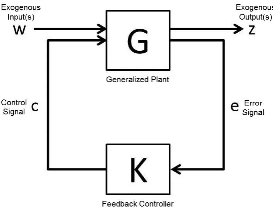
1.9 General model structure to form H∞ control problem . . . 17

1.10 Standard structure of the H∞ mixed sensitivity problem . . . 19

1.11 Control structures in the H∞ loop shaping method . . . 22

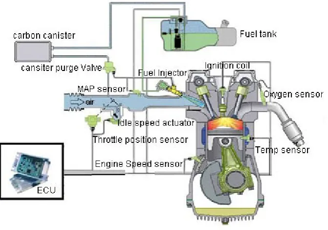
1.12 Modelling of the engine control system . . . 26

2.1 Linear fractional transform . . . 33

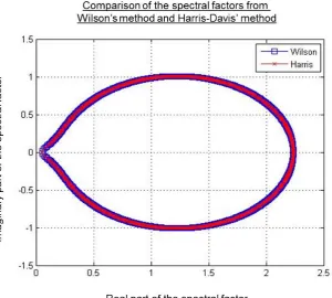
2.2 Comparison of the spectral factors from Wilson's and Harris-Davis' methods . . . 41

2.3 Disk Iteration method . . . 44

2.4 Program structure of the DI Method . . . 47

2.6 Two possible situations . . . 48

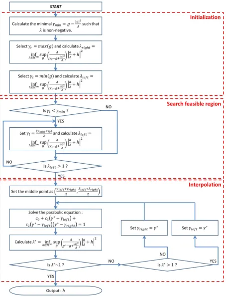
2.5 Procedure to choose γ∗ such thatλ∗ = 1 . . . 49

2.7 Procedure to search the feasible interval γlef t and γright . . . 50

2.8 Interpolation of γ∗ . . . 51

(10)

4.4 Convergence rate of Example 3 . . . 81 4.5 Deviation of the solutions in EX1 from dierent starting points . 82 4.6 Deviation of the solutions in EX2 from dierent starting points . 84 4.7 Deviation of the solutions in EX3 from dierent starting points . 85 5.1 The inuence of the discretisation number pto the computing time 93

5.2 System conguration with multiplicative uncertainty where the plantG = _s₊₁1 , the weighting function WI = 0₀._.125₀₃₁₂₅s+0_s₊₁.25 and the

controllerK . . . 96

5.3 Control system based in Figure 5.2 for the parametric controller design method . . . 96 5.4 Bode diagram of the primary sensitivity functionS1and the

weight-ing function 1/WS . . . 98

5.5 Bode diagram of the complementary sensitivity function T1 and

the weighting function 1/WT . . . 99

5.6 Step response simulation of the system in terms of T1 . . . 99

5.7 Comparison of the measured response (Blue) and the simulated response (Red) . . . 100 5.8 The uncertainty disk of the frequency response G(jω) . . . 101 5.9 The nonparametric controller design method . . . 102 5.10 Computation of the frequency response of the uncertain plant . . 102 5.11 Comparison of the measured frequency response (FRF) and the

average frequency response (FRF) . . . 103 5.12 Comparison of Bode diagram of the primary sensitivity function

S2 and the weighting function 1/WS . . . 105

5.13 Comparison of the complementary sensitivity function T2 and the

inverse of the weighting function WT . . . 106

5.14 The system step responses with the controllers K1 and K2 . . . . 106

6.1 Comparison of the solutions by dierent analytic function methods 110 6.2 Comparison of the sensitivity function S and T in their Bode

dia-grams . . . 112 6.3 Step responses of the controllers CDI, CN I ,and CLP . . . 113

6.4 Comparison of the frequency respons of the analytic solutions Q∗

by dierent methods . . . 114 6.5 Comparison of the sensitivity functions S and T in their Bode

diagrams . . . 116 6.6 Step responses of the controllers CDI, CN I ,and CLP . . . 117

(11)

301 Quadratic spline function . . . 132

401 A unimodal function f(x) in the interval [a, b] . . . 134

402 f1 and f2 in the interval [a, b] . . . 135

(12)

List of Tables

1.1.1 The RS conditions for dierent types of uncertainty . . . 12 2.2.1 Comparison of Wilson and Harris-Davis methods . . . 41 4.1.1 Results of Example 1 (256 points and the tolerance = 1E-6) . . . 76 4.2.1 Results of Example 2 (256 points and the tolerance = 1E-4) . . . 77 4.3.1 Results of Example 3 (256 points and the tolerance = 1E-6) . . . 77 4.4.1 Results of Example 1 (256 points and the tolerance = 1E-8) . . . 80 4.4.2 Numerical results in Example 3 . . . 81 6.4.1 Comparison of the dierent discretization numberspfor the S.I.S.O.

mixed sentivity control problem . . . 119 6.4.2 Comparison of dierent orders n for the SISO mixed sensitivity

(13)

Nomenclature

Notations

[a, b] Closed interval between a and b

¯

F Complex conjugate of the function F

∀ For all

∈ Belong to

C The eld of complex numbers CN The ring of N dimensionalC space

H1 The vector space (Hardy space) of complex-valued holomorphic

func-tions f bounded on the unit disk such that kfk

H1 = sup

θ

1 2π

´2π

0

f ejθ

dθ <∞

H2 The vector space (Hardy space) of complex-valued holomorphic

H2 = sup

θ

(₂1_π´₀2πf ejθ

2

dθ)1/2 _<_∞

H2(∂D) The set of the functions in H2 on the unit circle∂D

H1N The ring of N-dimensionalH1 space

H2N⊥ The orthogonal complement of the N-dimensionalH2 space H2N The ring of N-dimensionalH2 space

RH∞ The subspace of the real part ofH∞where functions are real-valued,

stable, and proper with real coecients

R The eld of real numbers

(14)

RN The ring of N dimensionalR space

H∞ The vector space (Hardy space) of complex-valued holomorphic

H∞ = sup

θ

f ejθ

<∞

H∞N The ring of N-dimensionalH

∞ _space

Ha Hankel operator with symbol a

L1 The Banach space of all measurable functionsf whose integral of the

absolute value is nite, i.e.

kfk_L

1 ≡

´∞

−∞|f|dω < ∞

L2 The Banach space of all measurable functions f whose square root

of integral of the square of the absolute values is nite, i.e.

kfk_L

2 ≡(

´∞ −∞|f|

2

dω)1/2 _<_∞_.

The L2 space is a Hilbert space.

L2(∂D) The set of the functions in L2 on the unit circle ∂D

a.e. Almost everywhere

G Transfer function of the plant K Transfer function of the controller

L The open-loop transfer function dened as L≡KG Q The noise sensitivity function dened asQ≡ K

1+KG S The primary sensitivity function dened as S ≡ 1

1+KG T The complementary sensitivity function dened as T ≡ KG

1+KG V The disturbance sensitivity function dened as V ≡ G

1+KG CTa Complex conjugate of Toeplitz operator with symbol a Q∗ The optimal noise sensitivity function

S∗ The optimal primary sensitivity function

(15)

V∗ The optimal disturbance sensitivity function

A/B The quotient space of a vector spaceA by a subspace B ∂D The boundary of the unit circle

<(F) Real part of the function F

A∗ Complex conjugate of transpose of the matrix A or the operatorA A−1 Inverse of the matrix A or the operatorA

AT Transpose of the matrixA

D The domain in the open unit circle In N ×N Identity matrix

j Square root of−1, i.e. j =√−1

s Laplace transform variable

Abbreviations

DI Disk Iteration method ECU Engine Control Unit

EMS Engine Management System L.H.P. Left Half Plane

LFT Linear Fractional Transform LP Linear Programming method LTI Linear Time Invariant

MBC Model-Based Control

MIMO Multiple-Input-Multiple-Output NI Newton Iteration method NP Nonparametric Method PPP Peak Pressure Position

(16)

R.H.P. Right Half Plane SA Spark Advance SI Spark-Ignition

SISO Single-Input-Single-Output SS State-Space

T Transpose

TDC Top Dead Centre TF Transfer Function

TWC Three Way Catalytic converter

(17)

(18)

Chapter 1 Introduction

Conventionally, to calibrate an engineering control system, the parametric iden-tication of the system plant is needed in the rst place in order to obtain its mathematical representation in the form of a model with a restricted (low) num-ber of parameters. Based on the mathematical model, the controller is then designed or computed to meet the performance requirements specied by the de-signer. The controller is practically implemented in the real system generally as a feedback system and the performance of the controlled system is then exam-ined and validated. This controller design approach is generally known as the Model-Based Control Method (MBC). However, the MBC method is, in practice, sensitive to the accuracy of the parametric model in the rst system identica-tion process. In addiidentica-tion, establishing a satisfactory model sometimes takes a long time and requires a priori knowledge. Controller design methods to poten-tially prevent a signicant mismatch between the model and the real system can be achieved by what are known as the Nonparametric (NP) methods. They have been developed on the basis of the input-output plant data in either the time or frequency domain. Because NP methods are more directly based on the exper-imental data, the controller has the potential to be more robust to the system modelling errors. Moreover, most of the performance requirements, such as band-width, and gain-phase margin in the frequency domain are able to be considered in the frequency-based NP methods. NP approaches are therefore potentially powerful for designing robust controllers in engineering systems. Nevetheless, only a few NP control design methods are available to date, which accordingly motivates the research work in this thesis to investigate and develop such NP methods.

(19)

engine, the ECU determines not only the amount of fuel and air intake into the engine chamber but also the spark timing to track the torque demand, the engine speed requirement, and control the other variables such as the temperature, emis-sions etc.. The control loops in the engine management system include those for most of the air-fuel ratio control, ignition control, idle speed control and knock control [35].

In this chapter, a literature review of feedback control theory is presented in Section 1.1. The H∞ feedback theory is also outlined in details in this section.

An introduction to the control loops in the automotive ECU are outlined in Section 1.2. Section 1.3 summarizes each chapter in the thesis. The contributions of the research work in this thesis are addressed in Section 1.4.

1.1 H

∞

Feedback Control

The controller design method formulated in terms of minimising the H∞ norm

is generally known as the H∞ control problem and addresses the issues of the

worst-case design for linear plants with unknown disturbances and unstructured plant uncertainties. The H∞ space of functions represents the Hardy space of

all functions which are analytic and bounded in the right half plane. The H∞

controller design method was initially formulated by Zames [104] as a mathemat-ical optimization problem in terms of the H∞ norm. In the 1980s, theoretical

work on approximation theory, functional analysis, operator theory and spectral factorization facilitated the optimal or sub-optimal controller designed by the

H∞ method in the frequency domain. The H∞ control theory was reviewed and

related to state-space means by Francis in [24] for nite-dimensional systems and by Foias in [23] for innite-dimensional systems. The research in the time do-main approach, which is based on the state-space representation of the system, motivated the development of H∞ optimal control theory by means of Riccati

equation solutions [21]. Many results and work by researchers have promoted the time domain H∞ approach to deal with more general control problem, e.g. the

time-variant control problem [6] and the nonlinear control problem[2].

Despite the fact that the state-space theory is relatively complete, theH∞

con-trol theory in frequency domain has several advantanges. One of the advantages of the frequency domain approach is that it can be deployed as a nonparamet-ric H∞ controller design method directly based on the output from an ecient

(20)

of a robust controller.

The frequency domain approach developed by Helton et al. [44, 47, 80] has been used in a sup-optimal nonparametricH∞controller design method for stable

plants in [106]. Helton et al's theory is based on nding analytic function solu-tions to the Nevanlinna-Pick interpolation problem [109] and the related operator theory [5, 9, 77]. The sub-optimal nonparametric method was also successfully applied to the engine fuelling control system problem in [107, 108]. In terms of Helton et al's approach, the method aims to solve the mixed sensitivity control problem using appropriate weighting functions. However, the method is restricted to convex problems where the local optimum is the global optimum. Furthermore, the interpolation to guarantee the internal stability requires the parametric iden-tication to allow computation of the Right-Half-Plane (RHP) poles and zeros.

Another nonparametric approach by means of parameterising the performance constraints in H∞ norm was developed by Karimi and coworkers in [27] and

summarized in [26, 56]. Karimi's method limits the selection of performance constraints in order to convexify the weighted sensitivity functions problem[56]. The application of his nonparametric method on a double-axis positioning system was presented in [57].

The other frequency domain approach of the Quantitative Feedback Theory (QFT) method was initiated by Horowitz [53]. This was adopted to a nonpara-metric method and applied to the automotive throttle control problem by A. Abass [1].

1.1.1 Feedback Control Theory

Two realizations of a Linear-Time-Invariant (LTI) physical system - the transfer function (TF) model and the state-space (SS) model - are introduced. Mathe-matically speaking, given the continuous input u(t)and output y(t), the transfer function H(s)is dened as the relationship between the Laplace transformL {·}

of the input u(s) and the output y(s) with the complex variable s, as denoted

H(s) = L {y(t)}

L {u(t)} = Y (s)

U(s) (1.1)

The Laplace transform maps a function in the time domain (e.g. u(t) and

y(t)) to the complex frequency domain . Mathematically, the substitutions=jω

connects the Laplace transform to Fourier transform. The transfer function model is possible to be estimated by using Fourier transform and is thereby commonly used in the frequency-domain approach of classical control theory.

(21)

describes the input-output relationship as a set of rst order dierential equations :

 



˙

x(t) = Ax(t) +Bu(t)

y(t) =Cx(t) +Du(t) (1.2) where u(t) ∈ _Rp _and _y₍_t₎ _∈

Rq are the p inputs and q outputs respectively, x(t) ∈ _Rm _{are the} _m _{state variables and} _A

m×m, Bm×p, Cq×m, Dq×p are the

system matrices.

The state-space model deals with functions in real time so the use of state space is viewed as the time-domain approach in the control theory. In addition, insight into the system (e.g. controllabilitiy, observability) is revealed by the state space realization even if the state variables are not related to physical meanings. The approach is also known to be numerically good for algorithms. As a result, there has been great interests in the development of the state-space approaches in recent years. Many applications in many control topics ( e.g. MIMO control prob-lems, nonlinear control ) have been extensively used the state-space formulation [44, 83].

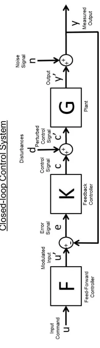
It is known that the purpose of control is to apply the control input to the plant to achieve desired output requirements. It is often straightforward to in-verse the model that describes the dynamics of the plant system. In this case, the inverse transfer function can be used as the controller in a form of 'open-loop control' as shown in Figure 1.1. The advantage of open-'open-loop control is its simplicity and low cost to implement in real systems. Nevertheless, there exists several unavoidable issues with open-loop control, such as nonzero steady-state errors, possible instability when distrubances are present, non-robustness to plant parameter variations or errors, and the external disturbances [25]. As a result, the alternative strategy of closed-loop control or feedback control can be used to cope with the above problems.

Figure 1.1: Structure of general open-loop control systems

(22)

troller K is fed to calculate the dierence e between the input signal u0 , which

is pre-processed by the pre-lterF, and the output y0, which contains the

distur-bancesdand the noisen. The closed-loop control not only solves the problems of

stability, robustness and reliability but also the capacity for more accurate track-ing performance when disturbances are present. Nevertheless, compared to the open loop control scheme, the closed loop control system may be more complex and require more costs on additional sensors.

From Figure 1.2, the following variable relationships can be established in frequency domain                           

u0 =u·F e=u0−y c=e·K c0 =c+d y0 =c0·G y=y0+n

(1.3)

and formulated in the compact form :

y0 =KGF[I +KG]−1·u+I[I+KG]−1·n+G[I+KG]−1d (1.4)

and

 



e=F [I+KG]−1·u−G[I+KG]−1·d−I[I+KG]−1·n

c=KF[I +KG]−1·u−KG[I+KG]−1·d−K[I+KG]−1·n (1.5)

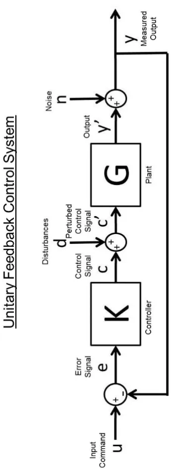
The unitary closed-loop control system can be obtained with a prelterF = 1. In this case, it can be observed from Equation 1.4 and 1.5 that the four sensitivity functions in the feedback control system are derived as

              

S =I[I+KG]−1 = [I+L]−1 Primary sensitivity function

T =KG[I+KG]−1 =L[I+L]−1 Complimentary sensitivity function

Q=K[I +KG]−1 =K[I+L]−1 Noise sensitivity function

V =G[I+KG]−1 =G[I+L]−1 Disturbance sensitivity function

(23)

[image:23.595.243.406.138.704.2]

(24)

These four sensitiviy functions are generally known as the Gang of Four [7], and they dominantly describe the dynamic characteristics of a control system. The primary sensitivity function S dened as the transfer function from u to y0. The complimentary sensitivity function T dened as the function from the

system's output y to the input command u provides the information about the

tracking performance to the commandu in the system.

It is worth noting that the equation

S+T =I (1.7)

is always true by the denitions of the functions S and T : S = I[I+L]−1 and

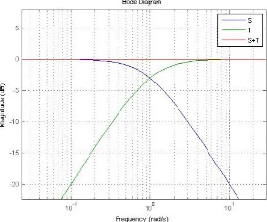
T =L[I+L]−1 1. It is important to notice that Equation 1.7 limits the design of the controller naturally because, in Equation 1.7, a compromise between the functions S and T is obviously required. In other words, attempting to seek

better tracking performance in T results in the less robustness to the noise n in S. The phenomenon is illustrated in terms of the corresponding Bode diagram

[image:24.595.182.454.403.629.2]

of S and T in Figure 1.3.

Figure 1.3: Bode diagram of the primary sensitivity function S = ₂_s22₊₅s+3_s₊₃ and

the complementary sensitivity function T = ₂_s22s₊₅2+3_s₊₃s

1

REMARK In the multiple-input-multiple-output (MIMO) systems, the right hand side of

(25)

1.1.2 Stability

The stability of the controlled system is a very important criterion in the controller synthesis since the unstable system may result in an unpredictable response. In the TF representation, it is known in the control theory [25, 62, 109] that if a linear continuous time-invariant system is to be stable, the roots of the closed-loop characteristic function I +L(s) = 0 ( i.e. the poles of the closed-loop system ) are all in the left half plane (L.H.P.). This is generally known as Routh-Hurwitz stability criterion. In the state space representation, the poles are usually computed as the roots of the characteristic equation det (sI−A) = 0 where s is

the Laplace variable and A is the matrix in Equation 1.2 [63].

In the feedback system shown in Figure 1.2, it is easy to derive from

Equation 1.4 and 1.5 that, if no pole or zero in the right half plane ( R.H.P. ) of

G cancels out the zero or pole of K in the R.H.P., the transfer functions S and T in Equation 1.6 must be stable [101]. That is, the system is internally stable

if and only if the four sensitivity functions S, T,Q and V are all stable. This is

summarized in the theorem [109]:

Theorem 1. If there is no unstable pole-zero cancellation inKG, the closed-loop

system is internally stable if and only if one of the four sensitivity functions is stable.

Simply speaking, the requirements for the internal stability conditions of a LTI feedback control system are expressed as [47]

• The complimentary sensitivity transfer function T is in _RH∞

• No R.H.P. pole of the plant G is cancelled by any R.H.P. zero of the

con-troller K.

• No R.H.P. zero of the plant G is cancelled by any R.H.P. pole of the

con-troller K.

where RH∞ here denotes the space of all rational transfer functions with real

coecients that have poles in L.H.P. ( i.e. stable )

1.1.3 Robustness

(26)

dif-structured uncertainty or undif-structured uncertainty. The dif-structured uncertainty is the representation of a known structure with some unknown perturbations in the parameters themselves, e.g. a percentage tolerance. The unstructured uncertainty, however, has less specic structure and is generally expressed as a global multiplier or addition of the gain at each frequnecy. The unstructured uncertainty is not accounted for in the system identication stage, especially in the high frequencies range. Details about representations of structured uncer-tainty and unstructured ceruncer-tainty are referred to several books and publications [20, 83, 109]. In this thesis, only unstructured uncertainty is considered.

Two common representations of the unstructured uncertainty are shown in Figure 1.4.The additive uncertainty structure shown in Figure 1.4a leads to the form of the perturbed plant G = G0 +4 , where G0 is the nominal plant and

∆ represents the dierence between the real dynamics and the nominal model, i.e. the unmodelled synamics. In Figure 1.4b, the multiplicative uncertainty model is formulated in terms of Gas G=G0(I+ ∆). Both of the unstructured

uncertainty models are commonly used and widely discussed in various papers and books [20, 83, 109]. The relationship between the unstructured uncertainty models and the conditions for the robustness is discussed in the following.

It is known that the stability condition of closed-loop systems is inuenced by the uncertainty. The Small Gain Theorem by Zames [103], which is based on the feedback structure shown in Figure 1.5 whereG1 and G2 are the LTI transfer

functions, implies that the system performance is constrained to some extent by the uncertainty.

Theorem 2. In Figure 1.5, if G1 and G2 are stable, the system is stable if

kG1G2k∞<1 (1.8)

and

(27)

(a) Model structure of the additive uncertainty representation

(b) Model structure of the multiplicative uncertainty representation

(28)

Figure 1.5: Positive Feedback Control to explain Small Gain Theorem

Consider the structure of the feedback control system with the additive un-certainty model in Figure 1.4a, we can easily derive the transfer function from signal cto signal d as

Tcd =K[I +KG]

−1

In other words, the uncertaint system in Figure 1.4a is equivalent to the sytem in Figure 1.6.

Figure 1.6: Equivalent feedback control system for the Small Gain Theorem Let G1 =4, Tcd is viewed as G2 in Figure 1.5. By the Small Gain Theorem,

we then have

Theorem 3. For a stable uncertainty set 4, the closed loop system is stable if

4 ·K[I+KG] −1

∞ <1 and

K[I+KG]

−1_{· 4}

∞ <1

i.e.

K[I+KG] −1

∞ <

1

k4k_∞ (1.10)

(29)

weighting function on ₄¯_{, we can reform Inequality 1.10 as}

W ·K[I+KG] −1

_∞=kW ·Qk_∞ <

1

4¯

_∞

= 1 (1.11)

For the multiplicative uncertainty model, by the Small Gain Theorem, the stability condition for the feedback control system becomes

KG[I +KG] −1

_∞ <

1

k4k_∞ (1.12)

i.e.

W ·KG[I +KG] −1

∞ =kW ·Tk∞<

1

4¯

_∞

= 1 (1.13) The inequalities 1.11 and 1.13 are known as Robust Stability (RS) conditions. Table 1.1.1 lists the Robust Stability (RS) conditions for dierent types of un-certainty models. The derivations of these types of unun-certainty models are well known in many texts e.g. [18]

Uncertainty Plant Gp Robust Stability (RS) conditions Gp =G·[1 +4 ·W]

W · KG

I+KG

∞=kW ·Tk∞≤1

Gp =G+4 ·W

W · _I₊K_KG

∞ =kW ·Qk∞ ≤1

Gp =G·[I +4 ·W ·G]

−1

W · _I₊G_KG

∞ =kW ·Vk∞ ≤1

Gp =G·[1 +4 ·W]

−1

W · _I₊I_KG

∞ =kW ·Sk∞ ≤1

Table 1.1.1: The RS conditions for dierent types of uncertainty

1.1.4 H

∞

Control

The robustness is an important topic in the control system design. A well designed control system often results in good command tracking performance despite the unmodelled dynamics and the environmental disturbances. Robustness has been a dominantly inuential topic in system control theory in the 1960s and 1970s.

H∞ optimal control theory was then developed in the early 1980s when Zames

[104] considered a control problem as an optimization in terms of H∞ norm to

minimize the disturbance insensitivity in feedback systems. Since then, many eorts on developing the H∞ control theory were made by researchers. The

theory was soon recognized to deal with more constraints, such as robustness to modelling errors and other performance requirements. TheH∞method developed

by Helton et al. is systematic and extensible to more general control problems with classical control theory [47]. The extension of the H∞ control theory to

(30)

in recent years. Several textbooks [24, 83, 109] introduce the theory of the H∞

method as well as their applications. In this section, the background of the H∞

optimal control theory is described.

In general, the guidelines to design a robust control system are described as follows :

For the closed-loop system in Figure 1.7, in terms of the sensitivity functions

S, T, U, it is claimed that

• For the purpose of disturbance rejection, S to be small. • For the purpose of noise attenuation, T to be small.

• For the purpose of reference tracking, T to be close to identity. • For the purpose of control eort minimization,Q to be small.

• For the purpose of maintaining robust stability,Q to be small for the

addi-tive uncertainty model or T to be small for the multiplicative uncertainty

model.

It is observed that the requirements for disturbance rejection and noise attenu-ation are in conict because Equattenu-ation 1.7 : S +T = 1 must be satised. This requires a o which is fundamental to closed loop systems and the trade-o is generally achieved by making T small at high frequency and S small at

low frequency, as shown in Figure 1.3. Moreover, to accomplish the reduction of the disturbances in terms of the sensitivity functionS, the weighting function W_S−1 is selected to reects the desired shape of the function S. It is in general

required the function S is low at low frequencies as shown in Figure 1.8a. On

the other hand, since the complimentary sensitivity function T determines the

tracking performance and the robustness characteristic, the weighting function

W_T−1 is chosen to shape the function T to keep it near unity at low frequencies

and as low as possible to reject the noise at high frequencies in Figure 1.8b. It is therefore known that these requirements on S and T (and sometimes on Q) can

be viewed as the design specications equivalent to the constraints of the design boundary.

It is further discussed that, assuming that the multiplicative uncertainty model represents the perturbation in the plant model G, the robust stability

condition leads to the rst constraint

(31)

[image:31.595.236.409.184.658.2]

(32)

i.e.

kTk_∞<|WT|

−1

,∀ω (1.15)

Thus, it can be known that the peak value of the function T is bounded by |WT|

−1_.

In addition, another important property of a closed loop system is the nominal performance (NP) requirement of the sensitivity function S [83]

kWS·Sk∞ <1,∀ω (1.16)

i.e.

kSk_∞<|WS|

−1 _(1.17)

This implies that the magnitude of S is bounded by |WS|

−1_{. Typical}

repre-sentations of the two constraints (RS and NP) are plotted in Figure 1.8a and Figure 1.8b respectively where the two weighting functionsWSandWT are viewed

as the upper bounds for S and T. The controlled system performance can thus

be tailored by properly choosing the weighting functions WT and WS so as to

achieve the desired performance.

The weight shaping problem is generally acknowledged as the key requirement to success in the H∞ control problem. The requirements in Equation 1.14 and

1.16 may be expressed in the stacked form as the so-called mixed sensitivity problem

"

WSS

WTT

#

_∞

<1 (1.18)

The minimization of the H∞ norm of the mixed sensitivity problem is

ad-dressed :

By rewriting WS and WT as a function of γ,

γ = min

Stabilizing K

"

WSS WTT

#

_∞

(1.19)

Moreover, not only the bounds WS and WT forS and T but also the boundWQ

(33)

(a)S and1/Ws

[image:33.595.122.522.174.385.2]

(b)T andWT

(34)

γ = min

Stabilizing K



 

WSS WTT WQQ



 

∞

(1.20)

This is generally known as the canonical form of the mixed sensitivity control problem2_{. The derivation of Equation 1.19 is presented below.}

Consider the system in Figure 1.9 and compare it with Figure 1.7, G is the

augmented plant model that consists of the nominal plant model and the uncer-tainty model ∆, K is the controller, the exogenous output from the system is z,

and the exogenous input signals w includes the input command u, disturbance

[image:34.595.180.454.315.526.2]

signal d and the noisen .

Figure 1.9: General model structure to form H∞ control problem 2

REMARK For mathematical convenience, the stacked specications provides an intuitive way to combine all the requirements. However, the procedure in fact sacrices the accu-racy of each specication. For example, if the Euclidean norm is used in the mixed sensitivity problem, we can rewrite Equation 1.18 as

WS·S WT ·T

∞ = max

q

|Ws·S|2+|WT·T|2<1

This is very similar to Equation 1.14 and 1.16. However, suppose |WS·S| =

|WT ·T| in the worst case, we have |WS·S| ≤0.707 and |WT ·T| ≤0.707.

Com-pared to the Equation 1.14 and 1.16, these two constraints are more stringent by a factor of 1/√2. However, because the choice of the weighting functions is exible,

(35)

In Figure 1.9, the control laws for such system are expressed as " z e # =G " w c # = "

G11 G12

G21 G22

# "

w

c

#

and

c=Ke

The transmission function Fzw between the exogenous output signal z and the

the exogenous input signalw is derived as

z= G11+G12K(I−G22·K)

−1

G21

w=Fzww (1.21)

In terms of the system in Figure 1.10, Equation 1.21 becomes

      zS zT zU e       = "

G11 G12

G21 G22

# " u c # (1.22) where

G11=

   WS 0 0  

, G12= 

 

−WSG WQ WTG





, G21 =I, G22=−G

The transmission function Fzw is then derived as

Fzw=G11+G12K(I−G22K)

−1

G21=



 

WS[I+GK]

−1

WQK[I+GK]

−1

WTGK[I +GK]

−1   =   

WSS WQQ WTT



 

(1.23) The term in Equation 1.23 may then be used to formulate the standardH∞mixed

sensitivity problem as

γ = min

Stabilizing K

kFzwk∞= min

Stabilizing K   

WSS WTT WQQ

   ∞

(36)

[image:36.595.161.474.155.688.2]

(37)

The algorithm proposed by Doyle et al. [21] to solve the above problem is summarized :

Theorem 4. In the standard form of a feedback control system in Figure 1.9, for the plant G with the state space realization of

  

 

˙

x(t) = Ax(t) +B1w(t) +B2c(t)

z(t) = C1x(t) +D11w(t) +D12c(t)

e(t) = C2x(t) +D21w(t) +D22c(t)

i.e. the generalized plant is G=



 

A B1 B2

C1 D11 D12

C2 D21 D22



 

with the following assumptions :

• (A, B2, C2)is stabilizable and detectable

• D12 and D21 have full rank

•

"

A−jωI B2

C1 D12

#

has full column rank for all ω

•

"

A−jωI B1

C2 D21

#

has full row rank for all ω

• D11= 0 and D22 = 0

there exists a stabilizing controller K such that, for a given positive number γ,

kFzwk∞< γ

if and only if

1. the solution X∞≥0 to the algebraic Riccati equation

ATX∞+X∞A+C₁TC1+X∞ γ−2B1B1T −B2B2T

X∞ = 0

is such that

Re λiA+ γ−2B1B1T −B2B2T

X∞

(38)

2. the solution Y∞ ≥0 to the algebraic Riccati equation

AY∞+Y∞AT +B1B1T +Y∞ γ−2C1TC1−C2TC2

Y∞= 0

is such that

Re λi

A+Y∞ γ−2C1C1T −C2C2T

<0,∀i

the spectral radius ρ(X∞Y∞)< γ2

The solution to the H∞ feedback controller is thus given by the solutions to

these two algebraic Riccati equations above by [83]

K(s) = −F∞(sI −A∞)−1Z∞L∞

where

F∞ = −B₂TX∞

Z∞ = I−γ−2Y∞X∞ −1

L∞ = −Y∞C2T

A∞ = A+γ−2B1B1TX∞+B2F∞+Z∞L∞C2

The program codes to implement the solution to the two Riccati equations are im-plemented in MATLAB Robust Control Toolbox [8], which reliably and eciently compute the solution to the Riccati equations for the H∞ controller.

In addition to the aboveH∞ approach based on solving the Riccati equations,

an alternative approach proposed by McFarlance and Glover [30, 66, 67] is known as H∞ loop-shaping method, which is based on the H∞ robust stabilization by

the classical loop shaping technique and has the great advantage that weighting functions do not need to be chosen. The design process of the H∞ loop-shaping

method is separated into two stages. Firstly, the open-loop plant Gol equipped

with a pre-compensatorW1 and a post-compensatorW2 as shown in Figure 1.11a

is given by [83]

Gol =W1GW2

The robust stabilization problem which is then addressed is to nd the stabilizing

(39)

(a) TheH∞ loop shaping procedure-1

(b) TheH∞ loop shaping procedure-2

(40)

" I K∞ #

(I−GolK∞) −1

M−1

_∞

≤−1

where is selected such that ≤max where max is dened as

−_max1 _,inf

" I K∞ #

(I−GolK∞)−1M−1

_∞

and Gol =M−1N where M, N ∈ H∞ are the normalized co-prime factors of Gol

and satises the Bezout identity equation

M ·M∗+N ·N∗ =I

Secondly, the implemented feedback controllerK is then computed by combining

the two weighting functions W1 and W2 with K∞ as shown in Figure 1.11b by

K =W1K∞W2

In contrast to the above state-space approaches, Helton et al.[47] proposed a systematic method to solve the H∞ control problem in the frequency domain.

The H∞ optimization problem in his approach mathematically views

Equation 1.20 as a minimax optimization problem. Such optimization problem can be written as

min Γ (ω, f(jω)) = min

StabilizingK    WSS WTT WU·U

   ∞ (1.24) = min

StabilizingKmaxjω (WSS, WTT, WUU) (1.25)

≤ γ∗ (1.26)

where Γ (ω, f(jω)) is the objective function which is dependant on the variables

f(jω) and ω , and f(jω) is any analytic function in the frequency domain (e.g.

S, T or Q).

Helton and Merino [47] proposed that the optimal solution to Equation 1.24 (the f term in Equation 1.24 is usually the primary sensitivity function T or

the noise sensitivity functionQ) provides the solution of the stabilizing controller

(41)

be implemented in the real system. This can be accomplished in the system identication process and by using model reduction techniques [29, 81].

Furthermore, the objective function Γ (ω, f(jω)) in Equation 1.24 is often converted to the function Γ ejθ_{, f e}jθ

on the unit circle. This is because the optimization problem in the ejθ _{domain can be treated as a Nevanlinna-Pick}

interpolation problem [71, 73] and solved by using the solution to the Nehari problem [70]. For scalar cases, the solution to the Nehari problem is known to be unique and available by [3, 4, 5]. For vector cases, the Nehari problem can be solved by Nehari commutant lifting formula [47, 69, 77]. As a result, Helton and Merino's method attempts to approximate the performance function Γ in Equation 1.24 to the quadratic form using the solution update fk+1 ₌ _fk ₊_th

given by

Γ z, fk+1 =gk+

N

X

i=1

2·Re ak_ihk_i+

N

X

i=1

δhk_i

2

(1.27)

where z is the set of sampling points on the unit circle, and gk _{= Γ} _{z, f}k

,

ak ₌ ∂

∂zΓ z, f k

, δ = _∂z∂∂2_z_¯Γ z, fk

The function Γ in Equation 1.27 by iterating to the closest circular form is then related to the Nehari problem. The solution to the H∞ optimization problem

is then possibly obtained. Then this sub-optimal solution is transformed to the frequency domain to sythesize the rational function of the controller. The algo-rithm and the approach for solving the H∞ problems is coded as a package in

Mathematica language and is available for academic use at [41].

Another algorithm proposed by Helton et al. [39] is based on the Newton Iteration (NI) method to solve the operator equations for optimality conditions. The solution is optimal to the original optimization problem and converges very quickly. However, the method is found to be sensitive to the initial points and may diverge as the iteration continues.

The two algorithms to solve the problem are therefore discussed respectively in more details in Chapter 2 and 3.

To take advantage of the fact that frequency responses may be used almost directly from the experimental data, Zhao et al [107] developed a sub-optimal nonparametric H∞approach based on Helton's approach [47] and applied this to

an automotive engine Peak-Pressure-Position ( P.P.P. ) control problem. In the extension of Zhao et al's frequency approach to MIMO systems, a norm called

H∞ Frobenius norm in [92], dened as

sup

ω

kG(jω)k = sup

ω

(42)

optimise MIMO systems using the maximum singular value norm, it can be used for the H∞ Frobenius norm for MIMO systems which has itself certain

advantages[92]. The H∞ Frobenius norm optimization approach can be adapted

to solve a form of the mixed sensitivity control problem, which allows better control over the elements of the closed loop transfer function matrices, such as allowing decoupling[108]. In particular, Helton's method was extended by Zhao [106] as sub-optimal nonparametric method to deal with M.I.M.O. control prob-lems and also implementeed on the application of the Torque-λdecoupling control

in the Engine Control Unit (ECU) [108].

1.2 Automotive Engine Control

The engine is the key part to generate the power to accelerate automotive vehi-cles. Nowadays, most vehicles are equipped with internal combustion (IC) engine because its superior thermal eciency and compactness of the systems. In the recent engine technology, gasoline and diesel engines are the most commonly used types of internal combustion engine systems in terms of dierent thermal cycles and fuel properties. The gasoline engine is degisned by means of the Otto cycle, which based on the four strokes : intake, compression, combustion and exhaust. The fuel in the gasoline engine is pre-mixed in the intake manifold and ignited by the spark plug in the combustion chamber. As a result, the gasoline engine is also known as the spark ignition (SI) engine. The diesel engine, however, is built according to Diesel cycle. The combustion in diesel engine is based on the self-ignition of the fuel. There is no spark plug in diesel engine but the engine itself has the same four strokes as the gasoline engine.

(43)

diagram of the system in Figure 1.12b.

In this section, four important control loops in the ECU are introduced in more detail : Air-Fuel Ratio Control, Ignition Control, Idle Speed Control, and Knock Control. In Chapter 6 of the thesis, to investigate the performances of the controllers by using dierent algorithms, one of the control loops, which determines the optimal spark advance (SA) in terms of the peak pressure positions (PPP) of the cylinders in order to generate the maximum brake torque (MBT) [76, 75], is used as an example.

(a) General gasoline engine control scheme [22]

[image:43.595.152.488.250.485.2]

(b) Block diagram of the engine control system

(44)

1.2.1 Air-Fuel Ratio Control

Air-fuel ratio control is one of the most important tasks in automotive engine control. It is known [59] that, for a Spark-Ignition (SI) engine, the stoichiometric mixture of the air and fuel for the combustion is typically 14.7:1. The index λ

dened as the value of the air/fuel ratio over 14.7 determines the eciency of the Three-Way-Catalytic (TWC) converter in removing hydrocarbon (HC), carbon monoxide (CO), and nitrogen oxide (NOx) emissions ( i.e. the system meets the emission regulations ifλ∼1) as well as the fuel economy and power generation. With even small (5%) devidents, there exist signicant pollutants, such as HC, CO, and NOx, in the exhaust gases. As a result, a good control strategy is required to determine the angle of electronic throttle to x the manifold absolute pressure (MAP), and mass air ow (MAF). In addition, the opening and closing times of the fuel injector is also the key to achieving good emission control. As a result, most modern vehicles are now equipped with the universal exhaust gas oxygen sensors (UEGO) located in the air-fuel control path. The UEGO device allows feedback control ofλand so greatly improves the performance ofλcontrol.

Furthermore, TWC converters are commonly installed to reduce of the pollutants by chemical deoxidation. Nevertheless, there exists a problem of the reduction of the TWC converter's eciency below the working temperature, which results in a high level of exhaust pollution. In summary, with the stringent regulations on vehicle emissions, the role of the air-fuel ratio controller in the ECU is an essential but a challenging problem for the automotive control engineers.

1.2.2 Ignition Control

(45)

1.2.3 Idle Speed Control

In powertrain control systems, the idle speed controller is an important compo-nent in the engine management system (EMS). A typical vehicle is known to consume about 30 percent of the fuel at idle in cities [55]. Hence, the control of the idle speed signicantly inuences the overall fuel economy. It is estimated that reducing 100 rpm at engine idle speed theoretically improves the fuel eciency for one mile per gallon in the standard Constant Volume Sample calculation [54]. However, engine stall limits the achievable fuel economy by increasing the necces-sary engine speed in idle speed conditions. Typically, the range of idle speed in most engines is about 600 rpm to 1,000 rpm. In the idle speed control loop, the amount of air and fuel is respectively determined by the opening of the electronic throttle valve and the fuel injection time. To maintain the engine speed at idle, the optimal ignition time is often calculated in terms of the maximum best torque (MBT).

1.2.4 Knock Control

Knock phenomenon results from a self-ignition behaviour that produces very high pressure and locally high temperatures in the engine. Knock sometimes leads to catastrophic consequences, such as the damage of the cylinder and the rim of the piston. As a result, it is important to adjust the control parameters to prevent knock when it occurs. The knock control strategy is usually to retard the spark advance or decrease the boost pressure of the turbocharger until the knock phenomenon disappears and then to gradually advance the SA and increase the boost pressure thereafter [82].

1.3 Overview of the Thesis

This thesis presents an analysis of the dierent analytic function methods used to solve nonparametric optimization problems in the H∞ method. The summary

of each chapter is outlined below.

Chapter 2 The chapter presents the review of the Disk Iteration (DI) method proposed by Helton and Merino [46] and its implementation. The optimization problem in the DI method is reviewed in Section 2.1 where the approximation to the original H∞optimization problem is summarized. The two nonparametric

(46)

problem by using the Nehari-commutant-lifting formula is also discussed in this section. The algorithm of the DI method and the implementation of the DI method are presented in the latter part of Section 2.2.

Chapter 3 This chapter re-states the theory of the Newton Iteration (NI) method proposed by Helton et al. [39] and proposes the Matlab implementa-tion of the NI method. In Secimplementa-tion 3.1, the optimality condiimplementa-tions of the H∞

optimization problem are presented. The operator equation in the NI method is stated in the start of Section 3.2 where the solution to the operator equation is re-produced from the results in [39]. In terms of the Newton iteration procedure, the implementation of the Jacobian operator approaches the optimal analytic solution to the H∞ optimization problem. Later in Section 3.2, the matrix

im-plementation of the two components as the Conjugate Toeplitz operator and the Shifted Hankel operator is presented. The update increment function is found by the inverse of the Jacobian operator in the NI method at the end of this chapter.

Chapter 4 The chapter shows three numerical examples to analyze the above two analytic function methods. The formulation of each example is described in the rst three sections of this chapter. The discussion of the DI and NI methods in terms of their convergence rate is addressed in Section 4.4. The nding of the NI method's property in the three examples is discussed in Section 4.5.

Chapter 5 This chapter studied a nonparametric method proposed by Helton and Sideris [40] in terms of the HadamardH∞- Frobenius norm in the mixed

sensi-tivity control. The nonparametric methods for the internal stability requirement are discussed at the begining of Section 5.2 where the Hadamard H∞- Frobenius

norm problem proposed by Diggelen and Glover [92] is also reformed for nonpara-metric control. The algorithm of the LP method is given in the same section. The linear programming optimization problem using Streit's algorithm [86] is re-viewed in Section 5.3. An example problem due to Skogestad and Postlethwaite [83] is used to investigate the nonparametric LP method in Section 5.4.

Chapter 6 This chapter presents an application of the nonparametricH∞

(47)

ana-lytic function methods. The analysis and comparison of these anaana-lytic function methods are summarized in Section 6.4.

Chapter 7 This chapter outlines the results presented in the previous chapters and proposes the future research direction of the work in this thesis.

1.4 Contributions of the Thesis

The claims to novelty in the thesis are

• The Matlab implementation of the DI method originally proposed by Helton

et al. [46] is presented for the purpose of comparison and analysis with other algorithms. The nonparametric spectral factorization methods by Wilson [99] and Harris and Davis [36] are also coded in Matlab and incorporated as part of the optimization code. Although the solution of the DI method is not optimal to the general H∞ optimization problem, the optimization

problem can be approached by iterating to the closest circular form and solved in terms of the Nehari problem. Thus, its sup-optimal solution is still useful for nonparametric control and, in the problems with circular performance function, an optimal solution is obtained. Since the original programs that implement the DI method were coded in Mathematica [41], for use in engineering applications, it is practically useful to integrate a Matlab version of the DI method as part of a controller design toolbox.

• An alternative nonparametric method known as Q-parameterization or

You-la-Kucera parameterization of sensitivity functions by the sensitivity func-tion Qcan be used in order to meet the internal stability conditions in the

feedback H∞ problem and to replace the parametric interpolation method

proposed by Helton et al. [47, 106]. The interpolation method with the DI method has previously been implemented on an automotive engine control problem by using the FrobeniusH∞ norm [108], however, this interpolation

method required the parametric identication of the RHP pole and zero of the plant. The Q-parameterization method skips this parametric identica-tion process and thereby allows the approach to become fully nonparamet-ric method. In this thesis, the Q-parameterization method is successfully applied to an automotive engine control problem with nonparametric opti-mization algorithms.

(48)

method, the NI method is capable of dealing with multiple function op-timization with non-circular type objective functions. The solution by the NI method is potentially optimal to the general optimization problem. Fur-thermore, the NI method should in principle converge quickly to the optimal solution due to its second order convergence rate. These properties of the NI method potentially save cost in computing eort during the optimization process as well as improving the accuracy of the solution. The NI method is therefore more suitable for general nonparametric control problems. The NI method is also implemented in Matlab in this thesis for the purpose of analysis and practical use. This implementation is the rst published implementation of this important algorithm.

• The comparative analysis of the DI method and the NI method is presented.

This is the rst independent comparison of these two methods. The analytic solutions by both methods are investigated by applying to several numerical examples.

• A nonparametric approach by Streit's [86] linear programming (LP) method

forH∞control problems is proposed. Compared to that the DI method and

the NI method which are both based on the computation of the Fourier co-ecients of frequency response function, the LP method is formed by the approximation of the analytic solution directly on the basis of the frequency response itself. The central optimization approach originally studied by Helton and Sideris [40] using Streit's method [86] is described in this the-sis. The implementation of Streit's algorithm is also coded in Matlab for practical use and for comparison purpose. An example of a SISO control problem with multiplicative uncertainty by this nonparametric approach is demonstrated.

• The nonparametric approach using the dierent analytic function methods,

(49)

Chapter 2 Disk Iteration Method for

H

∞

Optimization

The standardH∞control problem is often viewed as a mathematical optimization

problem. The optimization problem mentioned in Chapter 1 can be solved by the Disk Iteration (DI) method proposed by Helton and Merino [46, 47]. Most parts of this chapter are originated from the work of Helton and Merino[46, 47] and the programs to implement the DI method are also available in [41]. However, the Matlab implementation of the DI method is rstly accomplished for the purpose of comparison and practical use.

In this chapter, starting with the statement of the optimization problem and the transformation from the OP T eproblem to the OP T dproblem in

Section 2.1, the underlying theory and the implementation of the Disk Iteration (DI) algorithm are presented in more details in Section 2.2.

2.1 Optimization Problem

This section is the summary of the work on H∞ optimization in the frequency

domain by Helton et al in [37, 47] and in other related publications [38, 39, 40, 42, 43, 45, 46, 48]. In this section, the H∞ control problem in the frequency

(50)

Given a continuous positive-valued functionΓin_CN whereN is the dimension

of the problem, and a set of all the stable functions on the jω axis ( denotes as RH∞ , the space of all functions whose poles have negative parts. ), nd the

optimal function f∗(jω)∈_RH∞ _{such that}

γ = inf

f∈RH∞

sup

ω

Γ (ω, f(jω)) (2.1)

where ω represents the frequency, and f(jω) is the frequency response function This problem is known as the OP T problem in [48]. It can be translated into

an optimization problem that searches the stabilizing controller in terms of the measureγ in the worst performance case.

In mathematical analysis, the functions are often treated on the unit disk rather than in the complex plane because of the use of the Fourier Transform, the ease of implementation in the computer codes and other properties in complex analysis. The transformation from the imaginary axis to the unit circle ∂D is

possible via a Linear Fractional Transform (LFT). A LFT is a one-to-one, linear, and bounded mapping in this case from the imaginary axis ( s = jω ) onto

the unit circle ∂D. It transforms the poles and zeros of the function in the left

half plane onto a point inside the unit cirle and maps the poles and zeros of the function in the right half plane onto the point outside the unit circle. The sampling points on the imaginary axis ( e.g.. jω ) are thus mapped to points on

the unit circle∂D by the linear fractional transform, as illustrated in Figure 2.1.

Figure 2.1: Linear fractional transform

Thus by means of the linear fractional transform, the functionf(jω)in_RH∞ in theOP T problem is mapped to the functionf ejθ

(51)

of all analytic functions f ejθthat are bounded and continuous in the unit disk D. The OP T problem is therefore transformed to the so-called OP T e problem

given by

OPTe Given a continuous, real, positive valued function Γ in D, nd the

optimal function f∗ ejθ

such that

γ∗ = inf

f∗_∈

A

sup

ω

Γ ejθ, f∗ ejθ= inf

f∗_∈

A

Γ ejθ, f∗ ejθ

_∞ (2.2)

where ejθ are the points spaced around the unit circle, f ejθ is

con-tinuous in H∞ and ∗ denotes the function value at the optimum.

For simplicity, we will denote z = ejθ _{in the rest of the thesis. It is stated in}

[45] that the OP T e problem is closely related to the sub-optimization problem OP T cproblem in terms of the sublevel setSθ(c) = {Γ (z, f (z))≤c, c∈R+}with

a prescribed performance function c∈_R+ :

OPTc Find f∗(z)∈_A with Γ (z, f(z))≤c, ∀θ,and c∈_R+such that

γ∗ = inf

f∗_∈

A

kΓ (z, f∗(z))k_∞= inf

f∗_∈

A

kk(z)−f∗(z)k2_∞ ≤c (2.3)

where k(z) is any complex-valued function

It is also shown in [45] that the sublevel sets Sθ have the shape of disk and

their properties of boundness, simple connectness, smoothness and convexity are closely related to the properties of solutions to the OP T e problem. Therefore,

the solution to the OP T c problem can be viewed as the solution to the OP T

problem.

Furthermore, in [46, 47], the generalization of the above OP T c problem for N ≥1 is considered :

OPTd Given the positive continuous functions w(z) and k(z), nd f(z) ∈ H∞N such that

γ = inf

f∈_H∞

N

sup

θ

Γ (z, f(z)) = inf

f∈_H∞sup

θ N

X

i=1

wj(z)|ki(z)−fi(z)|

2 _(2.4)

Two examples to illustrate the relationship between the OP Tdand the OP T c

(52)

Example1 [47] Given a scalar-valued function ( i.e. theOP T dproblem forN = 1)

Γ (z, f) = w(z)|k(z)−f(z)|2 (2.5)

= (2 + cosθ)

1

z+ 0.5−f

2 (2.6) ≤ γ

it is seen that the solution must lie in the disk centred at 1

z+0.5 with the radius

p

γ/(2 + cosθ). This can be related to theOP T cproblem by observing that the

sublevel sets of the solutions f are

f =f ∈_H∞;|k−f|2 ≤r2,for r∈_R+

where the centre function k = _z₊₀1_.₅ and the radius function r=pγ/(2 + cosθ). Consequently, the equivalent OP T c problem for this objective function Γ (z, f) can be reformed as

inf

f∈H∞

sup

θ

Γ (z, f) = inf

f∈H∞

sup

θ

(2 + cosθ)

1

z+ 0.5 −f

2 (2.7) = inf

f∈_H∞sup

θ k− ˜ f 2 (2.8)

where k =pγ/(2 + cosθ)

−1/2

· 1

z+0.5 and f˜=

_p

γ/(2 + cosθ)

−1/2

f

As the OP T cproblem is solvable by solving the Nehari problem, we

immedi-ately have the solution to the optimization for this type of Γ (z, f).

Example2 [47] An objective function that has more than one term of the form :

Γ (z, f) = w1|f|2+w2|1−f|2 ≤γ (2.9)

it can be considered a quasi-circular problem. The sublevel sets of the function Γ (z, f) are fomulated as the disks centred at w2

w1+w2 with the radius

1 (w1+w2)

γ− w1w2

w1+w2

1/2

. Furthermore, the problem can be written in terms of

f =

(

f ∈_H∞;

w2

w1+w2

−f 2 ≤ 1

(w1 +w2)

γ− w1w2 w1+w2

)

This implies that the problem can be viewed as a circular problem with the centre function w2

w1+w2 and the radius function

1 (w1+w2)

γ− w1w2

w1+w2

1/2

(53)

There-fore, it is concluded that any function in the form of

Γ (z, f) =

N

X

i=1

wi(z)|ki(z)−fi(z)|2

is said to be a quasi-circular function, which is solvable by means of its equivalent circular form.

In summary, whether the function is circular or quasi-circular, the OP T d

problem can be solved by solving the equivalent OP T c problem in terms of the

solution to the Nehari problem. To deal with other functions that are not of circular or quasi-circular form, the approximation to the nearest circular function is performed. In the ANOPT package [41], the approximation is coded in terms of using an interpolation method. The interpolation method is discussed in depth in Section 2.2.

2.2 Disk Iteration Method

This section describes the Disk Iteration method that is presented by Helton and Merino in [46]. The Disk Iteration method was implemented for application to several control problems [106, 108] in a very computationally eective way. Computer code for the Disk Iteration method is available from the open source program ANOPT package in Mathematica [41].

It is valueable to translate the ANOPT programs into the Matlab language. Since most control engineering work is done in Matlab, a procedural version of the ANOPT package was currently not available before the work in this thesis.

This section outlines the underlying algorithm in the ANOPT package. Start-ing the OP T d problem in the previous Section 2.1 and the investigation of the

spectral factorization methods in Section 2.2.1, the solution to the OP T e