Testing the Theoretical Accuracy of Travel Choice Models Using Monte Carlo Simulation.

This is a repository copy of

Testing the Theoretical Accuracy of Travel Choice Models

Using Monte Carlo Simulation.

.

White Rose Research Online URL for this paper:

http://eprints.whiterose.ac.uk/2403/

Monograph:

Ortuzar, J.D. (1979) Testing the Theoretical Accuracy of Travel Choice Models Using

Monte Carlo Simulation. Working Paper. Institute of Transport Studies, University of

Leeds , Leeds, UK.

Working Paper 125

[email protected] https://eprints.whiterose.ac.uk/ Reuse

Unless indicated otherwise, fulltext items are protected by copyright with all rights reserved. The copyright exception in section 29 of the Copyright, Designs and Patents Act 1988 allows the making of a single copy solely for the purpose of non-commercial research or private study within the limits of fair dealing. The publisher or other rights-holder may allow further reproduction and re-use of this version - refer to the White Rose Research Online record for this item. Where records identify the publisher as the copyright holder, users can verify any specific terms of use on the publisher’s website.

Takedown

If you consider content in White Rose Research Online to be in breach of UK law, please notify us by

White Rose Research Online

http://eprints.whiterose.ac.uk/

Institute of Transport Studies

University of Leeds

This is an ITS Working Paper produced and published by the University of

Leeds. ITS Working Papers are intended to provide information and encourage

discussion on a topic in advance of formal publication. They represent only the

views of the authors, and do not necessarily reflect the views or approval of the

sponsors.

White Rose Repository URL for this paper:

http://eprints.whiterose.ac.uk/

2403/

Published paper

Ortuzar, J.D. (1979)

Testing the Theoretical Accuracy of Travel Choice Models

Using Monte Carlo Simulation.

Institute of Transport Studies, University of Leeds,

Working Paper 125

UNIVERSITY OF LEEDS

Institute for Transport Studies

ITS

Working

Paper

125

November

1979

TESTING THE THEORETICAL ACCURACY OF

TRAVEL CHOICE MODELS USING MONTE CARLO

SIMULATION

BY J. D. ORTUZAR

ITS

Working Papers are intended to provide information and encourage discussion on a topic in advance of formal publication. They represent only the views of the authors, and do not necessarily reflect the views or approval of the sponsors.

CONTENTS

Abstract

1. Introduction 1

2. The Generation of Random U t i l i t y Models

3. A t t r i b u t e C o r r e l a t i o n and Model S t r u c t u r e s

4.

The P r o b i t Model: S t r u c t u r e and Transformations

5 .

The Theoretical Accuracy o f A l t e r n a t i v e Logit Model S t r u c t u r e s

6 .

Conclusions

References

Acknowledgements

Figures

ABSTRACT

ORTUZAR,

J.

de D.

(1979)

Testing the theoretical accuracy of

travel choice models using Monte Carlo simulation. Leeds:

University of Leeds, Inst. Trans. Stud.,

WP

125 (unpublished)

In recent years a considerable advance has been made in

the construction of micro-travel demand models from choice

theoretic principles. Within random utility theory, the structure

of models

may

be shown to relate to the perceived similarity

between discrete choice alternatives, and this aspect may be

interpreted mathematically in terms of the correlation between

the components of random utility functions. Several possible

model structures have now been proposed, varying from the

multinomial logit model (uncorrelated) through the partly

correlated structures (hierarchical and cross-correlated logit

kctions) to the most general form of probit model which allows

an arbitrary variance-covariance matrix.

In this paper, these model structures are discussed using a

geometric interpretation of random utility theory, and the

possibility of invoking transformations on the general probit

model is examined. Monte Carlo simulation methods are then used

to investigate some aspects of the trade-off between the generality

and accuracy of correlated structures (the cross-correlated logit

model in particular) and the greater ease with which less consistent

structures may be implemented. In this way, the theoretical

accuracy of the multinomial logit model is assessed.

TESTING THE THEORETICAL ACCURACY OF TRAVEL

CHOICE MODELS USING MONTE CARLO SIMULATION

1. INTRODUCTION

I n recent y e a r s considerable i n t e r e s t has centred on t h e r e l a t i o n s h i p

between t h e s t r u c t u r e of a t r a v e l demand model and t h e behavioural

p r i n c i p l e s a s s o c i a t e d with its formation. This has a r i s e n not only

-

because of t h e need t o underpin models with a c o n s i s t e n t t h e o r e t i c a l

r a t i o n a l e , b u t a l s o from t h e recognition of s t r u c t u r a l ambiguities i n

e x i s t i n g models

-

a s , f o r example, with t h e r e l a t i v e p o s i t i o n s of

d i s t r i b u t i o n and modal s p l i t models i n t h e conventional planning system

-

which can give r i s e t o s i g n i f i c a n t l y d i f f e r e n t r e s u l t s i n p o l i c y a n a l y s i s

en-Akiva,

1974; Williams and Senior, 1977). One p a r t i c u l a r framework within which t h i s r e l a t i o n s h i p has been sought i s t h a t provided

by random u t i l i t y t h e o r y ( f o r a review, s e e Dcanencich and McFadden, 1975).

I n t h i s quanta1 choice theory i n d i v i d u a l s a r e considered t o a s s o c i a t e

with each member An; n = l ,

...,

N of a d i s c r e t e s e t of options A , a net u t i l i t y Un; n = l ,

...,

N, and t o s e l e c t t h a t member with t h e highest value of U. To account f o r i n t e r p e r s o n a l v a r i a t i o n i n t h e value of a t t r i b u t e s

incorporated i n t h e u t i l i t y f u n c t i o n s , a n d t h e i n f l u e n c e of unobserved

f a c t o r s , t h e modeller considers t h e v a r i a b l e s (U1,

...,

Un,

...,

UN) t o be randomly d i s t r i b u t e d over t h e population confronted by a choice. The

p r o b a b i l i t y P t h a t an i n d i v i d u a l with p a r t i c u l a r c h a r a c t e r i s t i c s s e l e c t s n

an a l t e r n a t i v e An i s t h e n simply expressed i n terms of t h e p r o b a b i l i t y

t h a t Un be g r e a t e r than those values associated with a l l o t h e r options.

A formal choice model may be derived when t h e d e n s i t y function

f ( U )

-

= f (U1,

. . .

,

U N ) of t h e u t i l i t y components i s s p e c i f i e d .

It has r e c e n t l y been recognised t h a t t h e a n a l y t i c s t r u c t u r e of a model

i s c r u c i a l l y r e l a t e d t o t h e interdependency, o r s t a t i s t i c a l c o r r e l a t i o n ,

between t h e u t i l i t y f u n c t i o n s a s s o c i a t e d with each a l t e r n a t i v e

-

t h a t i s ,

with t h e s t r u c t u r e of

f(U)

(Williams, 1977; Langdon 1976; Daly and

Zachary, 1978; McFadden, 1979). A s e t of formal models now e x i s t s which

accommodates varying degrees of " s i m i l a r i t y " o r c o r r e l a t i o n between

generated by uncorrelated distributions, through the hierarchical logit

model

(HI.,),

to the generalised probit function

(GP) with arbitrary

correlation, expressed in terms of a variance

-

covariance matrix.

Until recently application of the generalised probit model has

been restricted to a small number

(3

or

4)

of choice options (Haussman

and Wise, 1978

)

.

However by invoking the Clark approximation (Clark,

19611,

Daganzo et al

(1977)

have extended its practical range. In

spite of the advances in its applicability there appear to be many

practical cases in which (a) the model cannot cope (~aganzo,

1979),

or

(b) there is a need for a compromise between the generality it can

afford m d

the greater ease with which less consistent structures may

,

be implemented. One such compromise is the cross-correlated logit (CCL)

function (Williams,

1977).

which is a closed-form model containing

alternative

HL

functions as special cases.

In this paper we wish to examine some general themes such as the

relationship between certain utility functions and the structure of

travel choice models; the possibility of invoking transformations in

order to simplify models and derive conceptual links between them; the

theoretical accuracy of particular choice models, and the problems of

misspecification associated with model structures and utility functions.

More specifically, we wish to address the following questions:

i)

Is it possible to apply transformations in 'utility space' in order

to simplify 'symmetric' probit models and enable conceptual links

to be forged with the logit family?

ii) How serious is the absence of 'similarity effects' in the multi-

nomial logit model? In other words, how much is the well known

'independence

from irrelevant alternatives' (IIA) property of the

model an impediment in choice modelling?

iii) How good an approximation to a general function is the cross-

correlated logit model?

iv) What is the effect of misspecification of choice models with

respect to model structure and their utility components?

v)

Can any of the logit models display pathological response

properties, and is it possible to recognise their symptons at the

vi) Can we discriminate between contending model structures on the

basis of goodness of statistical fit, and the character of their

inherent elasticity parameters? In particular, does a

good

agreement to bese year data necessarily imply good response

characteristics?

It should be stressed at the outset that any reference to the

accuracy of a model will refer to its consistency with the underlying

theoretical rationale, and not necessarily to its appropriateness in

choice modelling.

-

In Section

2,

the basic principles of generating random utility

models are reviewed, a geometric interpretation of the theory is

presented, and the Monte Carlo method as a means for numerical

evaluation of choice models is outlined. The existence and implications

of correlation between the utility functions associated with different

alternatives are then examined in Section

3

and the various approaches

to its incorporation in choice models noted. In Section

4

we investigate

the possibility of invoking transfomations in utility space as a means

of simplifying the general probit model. Although conceptionally

appealing in terms of its links with MNL,

HL

and CCL structures, the

potential for implementing such transfomations does not, in general,

appear practicable.

The numerical tests to determine the theoretical accuracy of the

alternative logit structures in a general choice context are then

described in detail in Section

5.

2. THE GENERATION OF M D O M UTILITY MODELS

Formally, we can express the model generator equations of rando~

utility theory as follows:

P

=

Prob (Un > Unl

,V

Ant

EA)

n (2.1)

in which f(U) is the joint distribution function of (U1,

. . .

,

UN) and

Rn:

Un

L

Unt

vAnl EA

(2.3)

Un

L 0

(2.4)

In this paper we shall be concerned only with those cases in which a

trip is actually made. The non-negativity restriction (2.4) will thus

be considered inoperative. For the distribution functions considered

later this will involve a negligible inconsistency, which does not

affect the argument to be presented.

To derive an explicit probabilistic choice model we need to know

both the form of f(1) and

an expression for the utility functions in

terms of the attributes of alternatives in the set A.

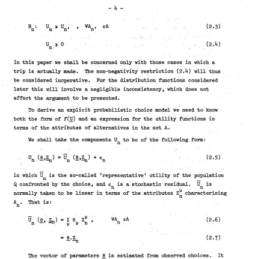
We shall take the components Un to be of the following form:

Un

=

un

(g.$)

+ E,

(2.5)

in which

is the so-called 'representative' utility of the population

n

_-

Q confronted by the choice, and

E~

is a stochastic residual. U is

n

normally taken to be linear in terms of the attributes

'

Z

characterising

n

A

.

That is:

n

The vector of parameters

g

is estimated from observed choices. It

remains to specify the distribution function f(g) or equivalently that

of the stochastic residuals

g .

A geometric interpretation of the theory may readily be derived

from expression (2.2).

In the utility space%&

bounded by the components

(U1,

. . .

,

U

)

,

the probability Pn is, for normalised f

(g),

the total

N

density of points in the region Rn bounded by the hyperplanes defined by:

and

U

=

U

V AneA

n

n'

This can be more easily seen in the convenient cartesian space. In

Figure l(a) we illustrate the fundamental utility distributions

[image:9.595.53.581.33.557.2]

distinguish those distributions g (U ) and g2(U )'which are associated

1 1

2

with the population

Q

confronted by the choice between alternatives

A1 and A2, from

gl(ul)

and

g2(u2)

which are the "choice specific"

distributions of utility, for those members of

Q

who have selected

options A1 and A2 respectively. The sum of these last two distributions

is termed the distribution of maximum utility g,(U), and the three

functions are formally defined as follows:

We shall also write the distribution of maximum utilities in the form

-

and we note here that the mean value of this distribution, U,, has great

significance in the evaluation problem (Williams,

1977).

The geometric interpretation of this simple choice process, which

is an extension of that provided by Robertson

(1977),

is given in Figure

l(b). For identical and independent distributions (IID), f(g) has a

-

circularly symmetric shape centred on and U2. The line OZ divides

1

the positive quadrant into the regions R1 and R2, and P1 and P2 comprise

of those corresponding portions of the distribution in these regions.

The distinction between g(U1) and the choice specific distribution g(U )

1 can readily be seen in terms of the respective projections onto the U

1 axis of the density function f(g), and that portion of f(g) bounded by

OZ

and the U1 axis. _I

An

important class of random utility models includes those generated

by IID utility distributions for which we can decompose

f(E)

as follows:

N

- 6 -

Here g(Un)

i s

t h e d i s t r i b u t i o n of t h e u t i l i t y component a s s o c i a t e d w i t h A

.

The expression f o r Pn can now b e w r i t t e n

n

h i s s i o n of t h e c o n s t r a i n t (2.4) allows t h e lower l i m i t s of

i n t e g r a t i o n t o be extended t o minus i n f i n i t y .

It i s by now widely known t h a t t h e much favoured multinomial l o g i t

model

(MNL)

i s an I I D model generated from Weibull (Gnedenko) p r o b a b i l i t y

d i s t r i b u t i o n s ( ~ h a r l e s Rivers Associates, 1972) f o r which

This i s a skewed unimodal d i s t r i b u t i o n , i n which t h e d i s p e r s i o n parameter

A i s inversely r e l a t e d t o t h e standard deviation, a , a s follows ( Cochrane

,

1975 ) :

Similarly simple p r o b i t models a r e generated from I I D Normal d i s t r i b u t i o n s .

For a number of s p e c i a l d i s t r i b u t i o n s , it i s possible t o evaluate

t h e i n t e g r a l (2.2) t o produce a n a l y t i c a l expressions f o r Pn, such a s t h e

MNL

i n equation (2.15). I n general, however, we have t o r e s o r t t o some

form of numerical method. One such approach involves Monte Carlo

simulation. A s f a r a s we a r e aware t h e first a p p l i c a t i o n of t h i s method

t o t h e s o l u t i o n of random u t i l i t y models i s t h a t of Albright, Lerman and

Manski (1977). i n t h e development of an estimation program f o r t h e g e n e r a l

p r o b i t model. However, and i n most cases independently, t h e power of t h e

approach has a t t r a c t e d numerous a p p l i c a t i o n s r e c e n t l y (Bonsall, 1979;

Chicago Area Transportation Study, 1979; Horowitz, 1978; Kreibich, 1979;

Manski and Lerman, 1978; Ortuzar, 1978; Robertson, 1977; Robertson and

Kennedy, 1979; W i l l i a m s and &uzar, 1979) but c l e a r l y its r o o t s can be

I n t h i s approach we follow t r a d i t i o n (~ammersley and Handscomb,

1965); a sample of s i z e S is c r e a t e d , and each ' i n d i v i d u a l ' member t ,

of S, i s confronted by t h e choice between A1,

...,

%.

Using a random number generator

a

set

of u t i l i t y values (U1,

.

.

.

,

u ~ ) is drawn from

f ( ~ ) ,

-

and t h e member

t

i s assigned t o t h a t option with t h e maximum a s s o c i a t e d u t i l i t y . For l a r g e S, t h e proportion Sn of ' i n d i v i d u a l s '

assigned t o option An w i l l approximate t o Pn, which i s given by

I n t h e simple Cartesian u t i l i t y plane examined before, t h e method

involves r a n d m sampling of p o i n t s from f(U1, U2). For a given sampled

t t

observation (U1. U 2 ) , t h e corresponding 'individual' w i l l be assigned

t o A1 o r

A2

according t o t h e region i n which t h e ' p o i n t ' may be found.

t

t

t t

if U > U2, i . e . (U1,U2) sR1, a s s i g n t o A1 1

(2.19)

t

t

t

t

if U < U2, i . e . (U1,u2) cR2, assign t o A2 1

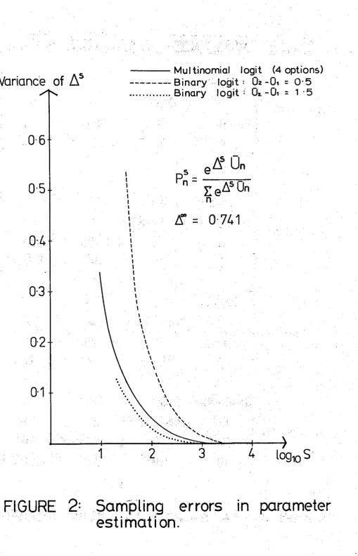
To t e s t t h e accuracy of t h e method with sample s i z e , t h e numerical

s o l u t i o n of a b o p t i o n l o g i t model was compared with t h e a n a l y t i c s o l u t i o n .

For a sample of s i z e S, t h e choice p r o b a b i l i t i e s P' were determined by n

drawing random values from four I I D Weibull f u n c t i o n s , with given means

-

- -

-

(ul, U2, U3, U q ) and standard d e v i a t i o n 0. Tnese numerically derived

p r o b a b i l i t i e s were then f i t t e d by a l o g i t function

S

i n which t h e parameter A was estimated by t h e usual maximum l i k e l i h o o d

method (Domencich and McFadden, 1975). I n Figure 2 , we show t h e empirically derived r e l a t i o n s h i p between t h e variance of A~ with t h e

s i z e of t h e sample S. I n order t o examine t h e accuracy of t h e numerical

s o l u t i o n under d i f f e r e n t c o n d i t i o n s , we repeated t h i s procedure f o r a

b i n a r y l o g i t model and d i f f e r e n t values of t h e d i f f e r e n c e between mean

u t i l i t i e s . A s it can be seen, t h e c l o s e r t h e options ( s m a l l e r d i f f e r e n c e

numerical t e s t s d e s c r i b e d i n later s e c t i o n s t h e sample s i z e was f i x e d

a t

S

=

30,000. (2

We now proceed t o consider more complex choice contexts i n which

t h e presence of c o r r e l a t i o n between u t i l i t y functions i s c e n t r a l t o t h e

s t r u c t u r a l develoment of t h e models.

3. ATTRIBUTE CORRELATION AM) MODEL

STRUCTURES

-

For t h e u t i l i t y d i s t r i b u t i o n s Un; n=l,

...,

N we can define a variance-covariance matrix & w i t h elements C _{given by:}

nn'

= E ( e n E ) V A n , A n t EA

n'

(3.1)

i n which E ( . ) denotes an expectation value. I n t h e c a s e of I I D u t i l i t y

components t h e matrix has, by c o n s t r u c t i o n , a simple diagonal form

where

I

_-

i s t h e u n i t m a t r i x of dinension N , and u t h e common standard d e v i a t i o n of t h e d i s t r i b u t i o n s g(U), t h a t i s

It i s one o f t h e i n t e n t i o n s of t h i s work t o determine t h e extent t o

which t h i s very simple s t r u c t u r e c o n s t i t u t e s a r e a l r e s t r i c t i o n t o choice

modelling.

The multinomial l o g i t ( Y ~ I L ) model (2.15) generated from I I D Weibull

d i s t r i b u t i o n s , which i s t h e r e f o r e c h a r a c t e r i s e d by a matrix with t h e

diagonal s t r u c t u r e ( 3 . 2 ) , has been very widely applied i n mode choice,

and nore r e c e n t l y d e s t i n a t i o n choice modelling ( f o r a review, s e e Spear

1977). It i s now well known, however, t h a t t h e model s u f f e r s a

r e s t r i c t i v e property o f c r o s s - s u b s t i t u t i o n , t h e 'independence from

irrelevant alternatives' ( I I A ) property, whereby the ratio

is independent of the utility values associated with other options.

The IIA property, once seen as a positive advantage to be exploited

in 'new option' situations, is now recognised to be a potential hazard

when certain alternatives are more 'similar' than others in the set A.

In random utility theory this notion of 'similarity' is interpreted in

tens of the presence of off-diagonal elements in the matrix

2.

_-

In certain applications, specific forms for the utility functions

tend to suggest themselves. Consider 'two dimensional' choice contexts

involving, for example, combinations of destination (D) and mode ( ! I ) .

Alternatives in each dimension will be denoted by (Dl,

.

,

D ,

...,

DN)

and

(y,

..

.

,X

.

.

..,:$*),

respectively, and the combination of m y

dimensions produces the 1P.J discrete choice options (Dl

5,

. .

.,

D

M

n m' ....Dd$l), which comprise the set A. The general element An is now

D

M

which might be a specific destination-mode combination for the

n m

purpose of performi~g an activity.

For such choice contexts we shall be particularly interested in

utility functions of the form

U(n,m)

=

U

+

U

+

Urn

n m

V

Dn!ImcA

(3.5)

here U and U may, for example, correspond to destination and mode

n m

specific utilities, respectively, while U might be the travel disutility

nm

associated with D

M

combination. This form was used in the shopping

n m

model developed by Ben Akiva

(1974),

and in a number of other applications

in the United States since that time.

Writing U(n,m) in terms of a 'representative' term b(n,m) and

a stochastic residual ~(n,m) we have

i n which

and

-

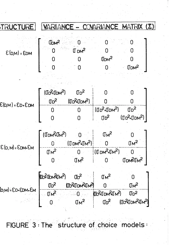
We s h a l l now assume t h a t t h e r e s i d u a l s E ~ ,E~ and E~ a r e s e p a r a t e l x

I I D , with

i n which 6 i s t h e Kronecker d e l t a . The elements of

_-

now become

and t h e matrix i s expressed i n Figure 3, t o g e t h e r with t h o s e corresponding

t o t h e r e s i d u a l s t r u c t u r e s

~ ( n , m )

=

cm

+

(3.13)

which a r e c l e a r l y s p e c i a l cases of t h a t defined i n Equation ( 3 . 8 ) . It

i s r e a d i l y seen t h a t t h e source of c o r r e l a t i o n i n 'multiple dimension'

cases i s t h e existence of a ccamnon term o r 'dimension s p e c i f i c ' element

we have developed i n Figure 3 ,

a

p i c t o r i a l r e p r e s e n t a t i o n of t h e s t r u c t u r e of t h e

z

-

matrix with c o r r e l a t i o n between a l t e r n a t i v e s incorporated through

common bonds

as

shown. This

i s

t h e b a s i s f o r a r e p r e s e n t a t i o n of t h e choice model i t s e l f (Williams, 1977). I n t h e f i r s t case both oD and oM

a r e zero and a diagonal

C

_-

matrix r e s u l t s . This case which i s c o n s i s t e n t

with Equation (3.11) w i l l correspond t o t h e

W L

model (2.15) i f t h e

u t i l i t y functions a r e drawn from I I D Weibull d i s t r i b u t i o n s . It i s c l e a r

t h a t t h e use of t h e u t i l i t y 'function ( 3 . 5 ) i n a KNL model of t h e form

(2.15) w i l l be i n c o n s i s t e n t because t h e a p p r o p r i a t e

z

-

matrix, corresponding

t o t h a t u t i l i t y function, i s not of t h e diagonal form involved i n t h e

generation of t h e model.

Before t r e a t i n g t h e more g e n e r a l case ( 3 . 8 ) , which i s c o n s i s t e n t

with t h e u t i l i t y f u n c t i o n

(3.5)

and which corresponds t o t h e f o u r t h

2

_-

matrix of Figure

3,

we s h a l l consider t h e d e r i v a t i o n of a h i e r a r c h i c a l o r nested model f r o m a f u n c t i o n c o n s i s t e n t with t h e r e s i d u a l s t r u c t u r e

and which corresponds t o t h e second r e p r e s e n t a t i o n i n Figure

3.

I n t h i s case t h e component o vanishes and t h e two parameters oD and oDM allow

_M

d i f f e r e n t degrees of c r o s s - s u b s t i t u t i o n between

intra

and

inter-

branch

a l t e r n a t i v e s i n t h e ' t r e e ' form shown i n Figure 3 ( b ) ; t h a t

is,

between

Dn Mm and DnMm,

,

i n t h e former c a s e , and between D ?I and D

,M

i n t h e n m n m'

l a t t e r . It may be shown (Williams, 1977) t h a t P(n,m), t h e p r o b a b i l i t y

of s e l e c t i n g D M can be w r i t t e n n m

P(n,m) = Pn.Pm (3.15)

i n which

and

Pn

=

Prob (Un

+

Unw

>

Unl

+

Unl+

,

Y

Dd ED)

(3.17)

with

If the components Urn are Weibull distributed variables

w(u.~~~,A)

with mean

if

+

y/A (where

y

is Euler's constant), and standard deviation

nm

K / ( ~ A

),

then it is readily shown (Cochrane,

1975)

that Un, is also

Weibull distributed, with mean

and standard deviation given by

The marginal distribution P is then derived from the sum of

n

Weibull distributed variables Un+ and variables Un, derived from some

distribution

r(~,<), n=l,

...,

N to be specified.

Now the hierarchical logit

(HL)

model (~illiams,

1977; Daly and

Zachary,

1978;

McFadden,

1979)

can be generated by specifying that r(~,&)

be that distribution of a

variate which is formed from the difference between random variables

-

₍₃₎

drawn from Weibull functions W(U,

En

+

tnr, 6) and W(U, Una,

A).

Because

Un and Un, are independent, the variance of their sum is

given by

... ... . . . . . . . . . .

..

... ... . . . . . .

...

.

. .

-

13

-

When uD = 0, the model collapses to the MNL, characterised by the

single parameter

A.

It can be seen that for a consistent model (and for

T(U,

5

_n ) to have a non-negative variance), we require (~illiams,

1977)

This condition is of particular importance, and its violation may

imply cross-elasticities of the wrong sign. Violation has, in fact,

been observed in conventional transport models (Williams and Senior,

1977).

We will come back to this concept later when discussing the pathological response properties of certain mis-specified models.

In the simulation tests to be described in Section

5,

in which the

model corresponding to Equation (3.8) is derived numerically, cn, cm

and E~~ will themselves be taken as Weibull functions, and it is necessary

to know what approximations are made if the resultant model is assumed

to be of HL form. In fact, the only approximation is involved in the

marginal probability Pn, because the sum of the two Weibull variates,

drawn from the distributions W(U,

Gn,,

A)

and W(U,

T,

n/(&-uD)) is

itself distributed Weibull.

For an example with

N

=

M

=

2, the parameters f? and

A

(the latter

should be exact) were estimated from the logit function (3.21) by

Maximum Likelihood, and their ratio was plotted against the standard

deviation u associated with the residuals E and compared with the

D n'

theoretical values in Equation (3.22). The results of this exercise

are shown in Figure

4.

It can be seen that a reasonably good

approximation is obtained.

We now turn to consider the choice model generated from the utility

function (3.5). Because of the form of the random residuals,

(3.8),

we can say immediately that this model should contain as special cases

the MNL and alternative HL functions. As far as the author is aware no

explicit analytic function has been obtained for such a structure.

Clearly one could appeal to the probit form and exploit the Clark

approximation (Clark,

1961),

but this would for medium size problems

still be unmanageable. Alternatively, we could try to exploit the very

symmetric structure of

Z

(as shown in Figure 3(d)) and attempt to

-

-

transform the probit model into an equivalent MNL model. In fact, this

will be the subject of the next section.

-

14

-

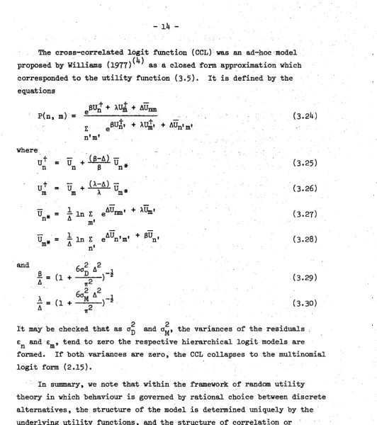
The cross-correlated logit function (CCL) was an ad-hoc model

proposed by Williams

(197'1')'~)

as a closed form approximation which

corresponded to the utility function (3.5).

It is defined by the

equations

where

-

t

-

(0-A)-

un

=

un

+

-

_B

'

n

*

U'f

=

-

_um

₊

-

(A-A)

-

m

x

'

m

*

2

2

It maybe checked that as uD and uM, the variances of the residuals

E

and cm, tend to zero the respective hierarchical logit models are

n

formed. If both variances are zero, the CCL collapses to the multinomial

logit form (2.15).

In summary, we note that within the framework of random utility

theory in which behaviour is governed by rational choice between discrete

alternatives, the structure of the model is determined uniquely by the

underlying utility functions, and the structure of correlation or

similarity between alternative choices is the essential feature which

dictates the complexity of the model. Varying degrees of similarity

[image:19.595.55.588.20.621.2]

may be accommodated within the logit family. The first three cases in

Figure 3 involve utility maximisations in which the variance-covariance

...

.

. .

...

...

...

...

...

.

.

.

...

.

.

,

... . . .

(4)

In that paper (section 5.3.2, pp 321-323), the function was denoted

General Choice Model. Mere recently, and in deference to the general

probit model and to the class of General Extreme Value (GEV) models

matrices -

g

a r e s p e c i a l cases of t h e cross-correlated s t r u c t u r e , with a

E

matrix and p i c t o r i a l r e p r e s e n t a t i o n summarised i n Figure 3 ( d ) . I n

-

-

Section 5 we w i l l p r e s e n t a s e t of simulation t e s t s on s t r u c t u r a l

m i s s p e c i f i c a t i o n designed t o examine some s p e c i f i c questions concerning

how good an approximation t o ( 3 . 5 ) i s t h e t h r e e parameters CCL model,

and what p o t e n t i a l e r r o r s can be introduced by using t h e s i n g l e parameter

MNL and two parameters HL models i n s t e a d . F i r s t , however, we w i l l examine

t h e general p r o b i t model and t h e scope f o r applying transformations i n

order t o produce more t r a c t a b l e models.

4.

THE GENERAL PROBIT MODEL, STRUCTURE AND !tWNSFORMATIOiYS

I n random u t i l i t y theory, t h e d e n s i t y f u n c t i o n which g e n e r a t e s t h e

general p r o b i t model (GP); f o r choice between N a l t e r n a t i v e s i s given by:

We s h a l l immediately transform Equation

( 4 . 1 )

from

g-

space i n t o

-

space using Equation ( 2 . 5 ) , giving

1

-N/2 - a T -1 1

f ( ~ ) =

-

(2n)

IgI

= P I - z g

&

5) ( 4 . 2 )

I f we define

-

-

-

Unnr

=

Un,

-

Un (4.3;

then r e s o r t i n g t o Equation ( 2 . 2 ) t h e model can be s t a t e d a s

-

-

-

Uln + En U2n + En

m

U ~ n + En

Pn

=

I I

...

I . . . I f ( g ) ( 4 . 4 )

-m -m -m -m

Although t h e GP(4.4) i s more general i n i t s t h e o r e t i c a l statement,

it i s considerably more cumbersome than t h e MNL o r HL t o implement. The

d i f f i c u l t i e s of achieving a s o l u t i o n t o t h e GP by d i r e c t n m e r i c a l

i n t e g r a t i o n f o r o t h e r t h a n 'small' problems, involving 3 o r

4

options

(Hausman and Wise, 1978) a r e w e l l known, and have l e d t o t h e formulation

of approximate s o l u t i o n schemes. One method involves Monte Carlo

The method is elegant, theoretically appealing and has the advantage

of being completely general, in the sense that in principle any function

can be integrated. However, it is not well suited for optimisation

purposes near the neighbourhood of the optimum, it is biased, and very

slow and expensive to use. (Bouthelier,

1978).

The second method, due to Daganzo et a1

(1977)

invokes the Clark

(1961)

approximation, which essentially involves the replacement of the

maxi

di

urn of bivariate normal variables by one normally distributed variable.

By repeated application of the Clark approximation, the multiple integral

in Equation

(4.4)

may be reduced to a particular univariate integral.

When the correlation between variables is non-negative, this approximation

which has been extensively examined by Manski and Lerman

(19781,

using

Monte Carlo simulation, is apparently accurate to a few per cent, for up

to 20 alternatives. However, problems with the possible existence of

multiple optima associated with the likelihood function of GP models, for

more than 2 alternatives, have recently been reported (Daganzo,

1979).

These imply that in general, there is no guarantee that the model can be

calibrated. The program and documentation of a powerful algorithm for

calibrating the GP model, using this method, are now widely available

(Daganzo and Schoenfeld

,

1978

)

.

When encountering normally distributed variables, it has often been

the case that a transformation to a co-ordinate system in which the

structure of variation in a data set is more appropriately described, has

provided not only insight into the nature of factors giving rise to the

variation, but has also formed the basis for approximation schemes.

hincipal component analysis is perhaps the best such example. (For a very

didactic treatment of transformation theory in multivariate analysis, see

Green and Carroll,

1976).

Moreover, it is well known that the MNL and

an uncorrelated, equal variance probit model (with suitably normalised

standard deviation) are almost indistinguishable. That is, if we could

transform general probit models into equivalent functions with diagonal

variance-covariance matrices, it might be possible to establish conceptual

links with the logit family, and in the process erase the burden of

numerical integration.

If this were not enough motivation, consider that the hierarchical

logit (3.21) may be written as-a MNL function with transformed utilities

The reader can check this by reorganising and using Equation

(3.19). In fact, this should not be too surprising, since McFadden

(1979)

has shown that any model derived from extreme value (Weibull) or

generalised extreme value functions may be written as an equivalent

multinomial logit model. In this group follow, for example, the hedonic

demand models developed recently by Charles Rivers Associates (Cordell

and Reddy,

1977).

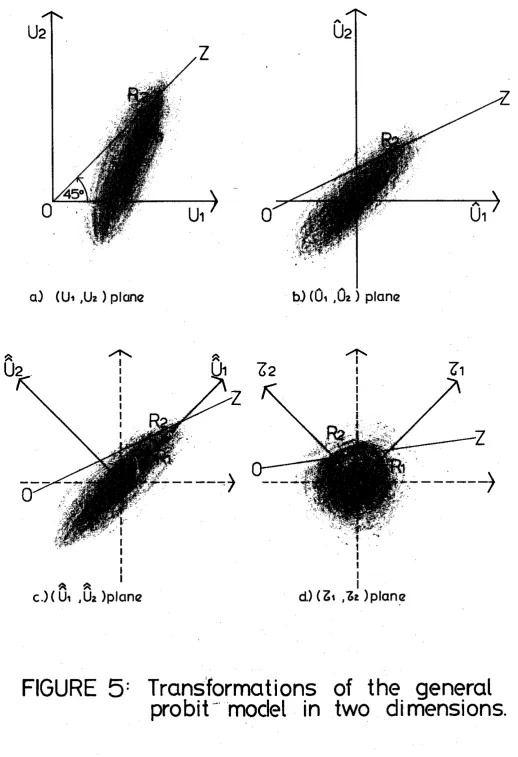
Let us first examine and illustrate the power of transformations in

the convenient cartesian two dimensional space.

Equation

(4.4)

reduces in two dimensions simply to:

where p is the coefficient of correlation, and

C

is given by

2

-

(4.7)

Figure 5(a) presents a pictorial representation of f(g) in g-space

for the general variance-covariance matrix

(4.7).

0 2 , the iso-utility

line, is defined by

0 2 :

u = u 2

1

(4.8)

and the region of integration R is defined by 1

Figure 5(b) presents a pictorial representation of the density function

..

[image:22.595.58.586.25.765.2]

-

18

-

In this transformed space the line

OZ,

which defines the region of

integration is given by

-

..

-

0 2 :

cru

+ U 2 = a U +U1

2

2

1 1 (4.11)

and consequently the region of integration is:

a

--

f

U1

d

-

Recall that we are searching for transformations that will restore the

symmetry of the independent case. The next move possible is to apply a

rotation in order to have the elipse-shaped density function oriented

along the new axes of the co-ordinate system. Figure 5(c) presents a

pictorial representation of the probability density function in this new

_..

space

fi

defined by

Notice that this transformation requires algebraic operations which

entangle the previous axes. The region of integration is this time

defined by:

- - a u l f m

The symmetry will be restored by a h t h e r compression of the axes.

It can easily be seen that this is achieved by:

..

..

Tl

=

U1 )

h-p

₎

1

z

1

(1.151

T2

=

u2 )

)

The corresponding pictorial representation is given in Figure 5(d), and

the region of integration is defined by

-OD 6T1 6 w

)

1

I$:

6 T2

s

h-p

(a1-a2) T f i 2 a 2 )

(hel6)

1

+

1

6

(a1+a2)

fl+p

(a1+a2)

Appendix 1 gives a matrix treatment of the problem, and shows

how the inverse of the variance-covariance matrix defining the quadratic

form of the bivariate normal is gradually transformed from the general

expression

to the simple expression of the independent equal variance model

after the three transformations defined by Equations

(4.10),

(4.13) and

(4.15).

Notice that because all the transformations are linear the iso-utility

line OC remains a line throughout; indeed it is given by

Now, the structural and numerical characteristics of the variance-

covariance matrix

C

_-

are dependent on the coordinate system (utility space)

-

20

-

form of t h e b a s i c problem i n t h e new space i n which t h e transformed

_-

matrix

-

i s

diagonal. We should not expect t h e b e n e f i t of an a n a l y t i c a l l y simpler d e n s i t y function t o be obtained a t zero c o s t , f o r t h e region

of i n t e g r a t i o n R over which An i s p r e f e r r e d i n Equation ( 2 . 2 ) , w i l l n'

a l s o be transformed.

I n general, under t h e t r a n s f o m a t i o n

t h e expression f o r P given i n Equation (2.2) n

becomes

i n which h(T) i s t h e transformed density function, J i s t h e Jacobian and

Rn, t h e new region of i n t e g r a t i o n .

In t h e p r o b i t model ( 4 . 4 ) , t h e algebraic manipulations and geometric

i n t e r p r e t a t i o n s of t h e required transformations a r e e s s e n t i a l l y t h o s e of

p r i n c i p a l component a n a l y s i s . The surfaces of constant d e n s i t y i n g-space

a r e t h i s time e l l i p s o i d s , given by t h e quadratic form.

T z-l

E = constant

Q F = E =

-

(4.22)

We wish t o invoke an orthogonal transformation

T

=

4 g

-

(4.23)

in which A1,

...,

AN

_{are the eigenvalues of}

_{C .}

_-

The eigenvalues and

corresponding eigenvectors are determined from the usual equation

Z v r =

A

fl

=

-

r - r

=

1,

...,

N

(4.25)

The quadratic form (4.22) may now be written

and the transformed probit model becomes

the Jacobian of the ~rthogonal'~) transformation being unity.

The transformed region of integration becomes

which is quite an unhospitable region involving all components of

T

on both sides of the inequality without possibilities of simplification,

-

and therefore rendering useless the effort to decompose the multivariate

density function

(4.1)

into the product of univariate functions (4.27).

Notice that this is not the case in the binomial context. Consider

equation

(4.6)

and define

...

. A .

. . .

...

... ... ... . . . . . . ..,

...

. . . . . .

(5)

Variance covariance matrices are especially well-behaved. They are

square, symmetric and positive semidefinite. All their eigenvalues are real and non-negative, the transformations that diagonalise them are orthogonal, and further, their inverse is equal to their transpose.

t h e n it can be seen t h a t Equation

(4.6)

reduces t o

t h a t i s , by means of t h e transformation (4.29) t h e m u l t i p l e i n t e g r a l

( 4 . 6 )

has been separated i n i t s two components,

and

el has been eliminated from

t h e upper l i m i t of i n t e g r a t i o n of t h e second i n t e g r a l . Note a l s o t h a t

i s p r e c i s e l y n2

,

t h e variance of t h e newly defined v a r i a b l e

n2

=

c2-el. "2

By making another transformation, namely

equation (4.30) f u r t h e r reduces t o :

where t h e f i r s t i n t e g r a l equals 1 and t h e second i s none o t h e r t h a n t h e

is very simple and efficient to use while still being completely general,

both in terms of correlation among alternatives and standard deviations

of the marginal distributions.

A

workable version of the model, along

these lines, but for three alternatives has recently been put forward by

Hausman and Wise

(1978).

Unfortunately, this method is also non-generalizable.

Before abandoning the transformation theory, let us examine probit _-

models corresponding to symmetric variance-covariance matrices, appropriate

to the utility functions.

I

and U(n,m)

=

Un

+

Um

+

Unm

as depicted in Figure 3. The block diagonal structure of

_-

in these cases

imply that the eigenvalues and eigenvectors of the matrix, will not mix

many utility components from the 'branch' associated with D and from

n

other branches. Although this occurs, there is a l s ~ considerable degeneracy

in the system characteristics, some eigenvalues being not unique. Consider

the model (3.14) in the simplest 2 x 2 case. The

-

matrix is given by

2

"D + 'DM 'D

0 0

C

=

-

-

(4.34)

0

0 0 u 2 aD2

+

OD

D

Solving for the eigenvalues

h

yields the equation

(4.35)

which simply reduces to

2

4

+{(a

+

'EM

-

u D l

= 0

-

D (4.36)

the degeneracy already apparent. The solution of Equation (4.35) is simply:

2 2

h1

=

2uD +

%

2

-

h2

=

'DM

(4.37)

I n conclusion, it has been shown t h a t it i s p o s s i b l e t o define

s u i t a b l e transformations t h a t allow one t o r e s t o r e t h e s i m p l i c i t j of

t h e integrand of independent equal variance models, t o a r j more general

function, although i n t h e case of models incorporating c o r r e l a t i o n

among many a l t e r n a t i v e s , t h e method does not commenrl i t s e l f because

t h e l i m i t s of i n t e g r a t i o n of Equation

( 4 . 4 )

become a f u n c t i o n of t h e u t i l i t i e s of s e v e r a l , if not a l l , t h e options. lieither does t h e method

work f o r simpler symmetric matrix s t r u c t u r e s , t h e problem tinis t i n e

being highlighted by t h e high degeneracy of t h e eigenvalues of t h e

matrix.

5.

THE THEORETICAL ACCURACY OF kLTERIIATITJE LOGIT 140D2L STFUCTJ3SS

I n Sections 2 and

3 ,

we o u t l i n e d a theory of choice behavio-a-,

random u t i l i t y theory. Within i t s framework t h e behaviour of i n i i - ~ i d u a l s

i s governed by r a t i o n a l decision-making among d i s c r e t e a l t e r n a t i - r e s ,

('homo economicus'), t h e s t r u c t u r e of models i s determine* uniq-iely by

t h e underpinning u t i l i t y f u n c t i o n s , and t h e s t r u c t u r e of c o r r e l a t i o n

or s i m i l a r i t y between a l t e r n a t i v e choices i s t h e e s s e n t i a l featlz-e which

d i c t a t e s t h e complexity of t h e model.

I f it i s accepted t h a t i n d i v i d u a l s s e l e c t a l t e r n a t i v e s and responrl

t o changes i n a manner which approximates t h e a s s m p t i o n s c f ti;:. t h ~ o r y ,

t h e r e a r e two immediate p r a c t i c a l consequences. F i r s t l y a s t h ~ tLree

model s t r u c t u r e s i n Figure 3 ( a ) , ( b ) and ( c ) , (!4!:L a r d two a l t e r n a t i v e

HL

models) a r e a l l s p e c i a l cases of t h e more general s t r ' i c t u r e i n Bigure

3 ( d ) ( i n which

oD,

oIq and aDM a r e a l l non-zero), any s t r 3 1 c t u r a l

ambiguity, a s r e f e r r e d t o e a r l i e r i n t h e paper, may be o b r i a t e i i f t h s

l a t e r model i s implemented.

Secondly, i f a p a r t i c u l a r model, say t h e h i e r a r c s i c a l s t r - ~ c t u r e is

Equation (3.21) is adopted f o r f o r e c a s t i n g demand response, t h e composite

u t i l i t i e s (3.19) and estimated e l a s t i c i t y paraueters 0 a n i A , m;st be c o n s i s t e n t with t h e t h e o r e t i c a l conditions underginning t h e r o d e l i . 5 .

s a t i s f y i n e q u a l i t y (3.23). It has been found i n S r i t i s h Trans?ort

Studies which have employed

a

HL of t h i s forn, t h a t e i t h e r condition

(3.19)

o r t h e parameter r e l a t i o n

0

d A have been v i o l a t e 8 . Tnese v i o l a t i o n s can give r i s e t o hyghly u n r e a l i s t i c respocse ? r o ? e r t i e s of

While a theory of model structure (and corresponding evaluation

measures (~illiams,

1977))

now exists which is consistent with rational

choice behaviour, there are many theoretical and practical issues which

remain to be resolved. The cross-correlated logit model or general

probit model appropriate to the utility structure (3.5) have yet to be

implemented, and it has been suggested that one should implement all

three special structures 3 . 1 1 ) (3.12) and (3.13) and select that which

yields the best statistical fit

g&

is consistent with the theoretical

conditions outlined in previous sections. (Ben Akiva,

1977;

Senior and

Williams,

1977).

It remains to assess the extent of mis-specification

involved in the implementation of a particular model in circumstances

for which a more general representation is appropriate. In this context,

Monte Carlo methods provide a very handy tool. (6)

We are now in a position to present a set of simulation tests on -

structural mis-specification which are designed to examine the following

questions:

(i) How good an approximation is the three parameter CCL model

to the exact model generated from Equation (3.5) through

utility maximisations?

(ii) What potential errors are made by invoking the single parameter

MNL and two parameter HL models, which accommodate restricted

degrees of similarity between alternatives, to an appropriate

[image:30.595.69.596.45.783.2]

three parameter specification?

Figure

6

depicts the experimental scheme. Data was generated by

direct simulation from utility functions of the form (3.5) for a simple

2 x 2 case.

A

whole range of models was tested, which can be

conveniently divided into two classes:

-

theoretical, i.e. with specified parameters based on

knowledge of the values of the underlying standard deviations;

-

calibrated, i.e. with parameters fitted by maximum likelihood.

The first class contains the four logit models discussed before

(MNL,

two alternative HL structures and CCL) and the second only the first

three.

(7)

Because the 'calibrated' versions always performed better

...

... ...

.

. .

...

...

... . . .

...

...

...

Williams and Ortuzar

(1979)

have used the method outlined here

to test the effects of theoretical mis-representation allowed by the relaxation of some of the assumptions associated with the decision process of 'homu-economicus'.

than the 'theoretical' we will consider only the former

from now on.

The simulated data sets consisted of the mean utilities and

aggregate shares of each alternative. The

MNL(~)

( 4

options) parameter

A

was estimated by maximum likelihood (using a Newton Raphson procedure

described in Appendix 2) and the EII,(l0) models were calibrated heuristically

and similarly as a series of binary logit models; the appropriate

composite utilities providing a link between the two levels in the

hierarchy.

Having estimated or theoretically determined the parameters of the

models for a given data set (base data), a second set of data was

generated for a particular change in the values of the mean utilities

-

new

-

Old

+

1)

consistent with the effects of a particular policy.

(say U = U r n

This second set, the 'design year data' was compared with the

predictions of the models for the same change in mean utility values.

By this means, the response properties of the models were also assessed.

The complete mechanism is depicted in Figure

6;

it can be seen that it

can easily be adapted to test not only structural mis-specification as

we did here, but more profound problems of theoretical mis-representation

(Williams and Ortuzar,

1979).

The simulation tests involved variation of the co-ordinates

(uD, uM, uDM).

A

standardisation or 'normalisation' condition to bound

the joint variation of these quantities, of the following form was used:

2

u2

+

o

+

u2

=

constant

D

M DM (5.1)

and a particular co-ordinate

(OD&

,

uM.

a uDM) corresponds to a particular a

simulation test. To illustrate the possible combinations of these three

quantities, we appealed to that property of equilateral triangles whereby

the sum of perpendicular distances to the three sides from an interior

( 8 ) The approximations involved in the models preventing the specified parameters to replicate the data as closely as the fitted parameters.

(9)

In

a

first set oftests the mean utility in Equation (2.15) was taken

as

U

=

U + U

+

Unm. In a second set of tests, we examined the

n m

effect of omitting a particular component, say by putting

&

= 0.

(10) In the first set of tests, the mean gtili* in the lower hierarchy

of Equation (3.21) was taken as U

=

Um

+

Unm (and correspondingly

-

Un

+

t,,

for the alternafive form). In the second set of tests the

..

-

_-

effect of omitting a particular component, say Um

=

0, could easily

point is a constant, equal to the height of the triangle. Any test

point may thus be identified with a point in or on the boundary of the

triangle, as shown in Figure 7(a). At interior points a three parameter

model (such as the CCL model) is necessary to capture the full range of

cross substitution implied by the utility function (3.5). On the

boundaries

CB

and

CA

the alternate HL models for which oM

=

0 and oD = 0

respectively, are appropriate (see Figures 3(b) and (c) ) . It is only

at the vertex C

(i

.e. oD

=

aM

=

0) that the MNL is an appropriate

specification.

In addition to test points randomly sampled from within the triangle,

four particular co-ordinate test points, as shown in Figure 7(b), were

selected for the presentation of results. Recall that in all tests two

alternatives were taken in each of the D and M dimensions, allowing a

four alternative choice model to be generated.

The general performance of the four models for these test points (11)

is shown in Figure 7(c). We have restricted ourselves to a comparative

quality assessment of the fit, in that it is the relative performance of

the models in which interest lies. (12)

A

visual display of the meaning

of this informal assessment, in the form of a particular set of base and

response results for the four models used to fit data generated from

test point 2 in Figure 7(b), is shown in Figure 7(d).

Under conditions of change, points in the second and fourth

quadrants of the right hand side of Figure 7(d) are deemed pathological

because the change in behaviour predicted by the model is opposite to

that simulated. We found that this behaviour is associated with the r

violation of the condition (3.23) in hierarchical logit specifications.

If, for example, oD >> oM, then the HL specification

MID

corresponding

to oM > oD will involve pathological behaviour. The condition, however,

(11) Results are shown for the first set of test only, i.e. when it

was assumed complete knowledge of the mean utilities. _I

(12) The performance measures used were average relative errors

(ARE)

I

defined as:

N

ARE

=

$

c

{

1

psim

-

?dl /?dl

i=l 1

-

xnd a izeasure, defined as :

appears also to depend on the underlying representative utility

values. (13)

If we further examine the performance of the models as reported

in Figure 7(c), we note that the CCL appears to be a good approximation

to the general fuuction

(3.5).

Its superiority to the other logit

forms was especially apparent when the three coordinates oD, uM and

u were different from zero and from each other. The most surprising

DM

and welcome outcome, however, was the remarkably robust performance

of the MNL, even at interior points of the triangle and especially when

uD uM. AS expected the IIA property was a considerable impediment

near the sides of the triangle, except in the immediate region of

point

C.

The last point to note in this section is, that out of the

estimated models (MNL and two HL forms), that with the best base fit

consistently provided a good estimate of the response to change:

this would seem to lend some theoretical/numerical support for the

suggestion of Ben Akiva

(1977)

that results of alternative

HL

and

MNL

models could be compared and the appropriate model selected

according to the estimated value of the 'similarity' parameter,

which in our notation is 6 / A .

We offer no apologies for the fact that the simulation tests

1

were confined to a 2 x

2

example

(4

options). We believe that the

1

results and conclusions in next section, would not be qualitatively

modified when the number of alternatives are increased, because the

structure of the variance-covariance matrix itself was the focus of the

mis-specification tests. The dependence of the results on the number

of options could, of course, be tested.

(14)

...

...

...

...

... ...

.

. .

...

...

.

.

.

...

...

(13) In the second series of tests the effect of omitting a

particular utility ccanponent

-

by putting

im

=

0, for example-

was determined. All results were inferior to their counterparts in the first series, as would be expected because the number of

'degrees of freedom' of the model specifications had been

reduced. The performance of HL (asymmetric in nature) was

particularly suspect and pathological behaviour became more

prevalant.

-

(14) More important, in exercises of this kind, is to make sure that the process converges. We found it was necessary to smple 30,000 observations to get consistent results. The reader is referred

6.

CONCLUSIONS

In this paper we have presented the essential features of random

utility theory, both formally and in a geometric framework which

provides a clear interpretation of the nature of choice.

We have studied the role of correlation and how the form of the

utility function uniquely determines the structure of models, their

complexity being dictated precisely by the structure of similarity

or correlaticnbetween the alternatives. In this way, we have been

able to present the basic assumptions of the most popular models,

multinomial logit, general probit and hierarchical logit, and

discuss their implications.

The general probit model is the more conceptually appealing

of model forms, although unfortunately the least tractable of them

for more than small problems, and even then with some yet unknown

properties. We have investigated the possibility of invoking

transformations in utility space as a means of simplifying it. We have

shown that it is indeed possible to define suitable transformations

that allow one to restore the simplicity of the integrand of independent

'equal variance' models to any more general model, although in the

case of models incorporating correlation among many alternatives,

what is gained on the joundabouts is lost on the swings because

of the non-separability of the multiple integral (4.27) which in

turn is due to the unhospitable form of the region of integration (4.28).

Although transformations certainly give more insight into the problem,

the potential for implementing them, even in the case of models with

symmetric variance-covariance matrices, does not appear practicable.

The results of the simulation tests are consistent with the

following conclusions:

i) The cross-correlatedlogit model is a good theoretical

approximation to the three parameter utility lunction

(3.5).

The superiority to other logit forms is especially apparent when

the standard deviations

oD,

oM and

oDM

are rather different from

zero and from each other. However its estimation is very complex

ii) The multinomial l o g i t model performs reasonably w e l l at

i n t e r i o r p o i n t s of t h e t r i a n g l e (indeed it i s considerably

more robust t h a n we had a n t i c i p a t e d ) and t h i s i s p a r t i c u l a r l y

t r u e when o

_D

-

oM. Its maximum e r r o r occurs near t h e s i d e s of t h e t r i a n g l e (except i n t h e immediate region of p o i n t C )

where t h e 'independence from i r r e l e v a n t a l t e r n a t i v e s '

property i s a considerable impediment.

iii) A good base f i t does not n e c e s s a r i l y imply a good response

model, after all every m o d e l k a l i b r a t e s ' . However, out of

t h e t h r e e a l t e r n a t i v e l o g i t s t r u c t u r e s (multinomial l o g i t and

two h i e r a r c h i c a l l o g i t forms), t h e model which provides t h e

b e s t base f i t provides a good estimate of t h e response t o change.

i v ) A mis-specified model ( t y p i c a l case i s t h e i n a p p r o p r i a t e

h i e r a r c h i c a l l o g i t form) w i l l tend t o display pathological

behaviour i n a response context. However it i s p o s s i b l e t o

recognise t h e symptoms a t t h e c a l i b r a t i o n s t a g e , by examining

t h e consistency conditions (eg. r u l e ( 3 . 2 3 ) ) .

I n t h e s e t e s t s we examined t h e c a p a b i l i t y of extended members

of t h e l o g i t family t o accomodate t h e s t r u c t u r e of s i m i l a r i t y between

a l t e r n a t i v e s embodied i n t h e u t i l i t y function ( 3 . 5 ) . The general

p r o b i t function would be a p p r o p r i a t e i n t h i s ' case, and indeed t o more

general u t i l i t y forms. Horowitz (1978) h a s , i n f a c t , examineQthe

p o t e n t i a l mis-specification problems of t h e multinomial l o g i t model

when compared with a

3-

a l t e r n a t i v e p r o b i t model. H i s r e s u l t s a r e complementary and c o n s i s t e n t with ours, i n t h e sense t h a t i n moat

p r a c t i c a l c a s e s , t h e g r e a t e r ease with which l e s s c o n s i s t e n t s t r u c t u r e s

-

provided t h e y a r e robust enough t o cope r e l a t i v e l y well with not s e r i o u s

mis-specification -may be implemented, w i l l win t h e day.

F i n a l l y t h e powerful t o o l employed i n our a n a l y s i s , Monte Carlo

simulation, deserves an e s p e c i a l word of p r a i s e . We noted t h e increasing

a p p l i c a t i o n of t h e method i n t h e t r a n s p o r t f i e l d , but we b e l i e v e t h a t

our p a r t i c u l a r use h e r e , c r e a t i n g a r t i f i c i a l d a t a s e t s on which t h e

e f f e c t s of s p e c i f i c model mis-specifications can be t e s t e d i n a c o n t r o l l e d

manner, i n d i c a t e s one way ahead t o a t t a c k t h e problem of model evaluation.

Indeed, it has a l r e a d y been u:ed i n a more ambitious p r o j e c t t o t e s t f o r

t h e o r e t i c a l misrepresentation and t o a s s e s s t h e v a l i d i t y of cross-sectional