This is a repository copy of Levy processes - from probability theory to finance and
quantum groups.
White Rose Research Online URL for this paper:
http://eprints.whiterose.ac.uk/9794/
Article:
Applebaum, D. (2004) Levy processes - from probability theory to finance and quantum
groups. Notices of the American Mathematical Society, 51 (11). pp. 1336-1347. ISSN
0002-9920
[email protected]
https://eprints.whiterose.ac.uk/
Reuse
Unless indicated otherwise, fulltext items are protected by copyright with all rights reserved. The copyright
exception in section 29 of the Copyright, Designs and Patents Act 1988 allows the making of a single copy
solely for the purpose of non-commercial research or private study within the limits of fair dealing. The
publisher or other rights-holder may allow further reproduction and re-use of this version - refer to the White
Rose Research Online record for this item. Where records identify the publisher as the copyright holder,
users can verify any specific terms of use on the publisher’s website.
Takedown
If you consider content in White Rose Research Online to be in breach of UK law, please notify us by
Lévy Processes—From
Probability to Finance
and Quantum Groups
David Applebaum
T
he theory of stochastic processes was one of the most important mathematical developments of the twentieth century. Intuitively, it aims to model the interac-tion of “chance” with “time”. The tools with which this is made precise were provided by the great Russian mathematician A. N. Kolmogorov in the 1930s. He realized that probability can be rigorously founded on measure theory, and then a stochastic process is a family of random variables (X(t), t≥0) defined on a probability space (Ω,F, P) and taking values in a measurable space (E,E). Here Ωis a set (the sample space of possible out-comes), Fis a σ-algebra of subsets of Ω(the events), and Pis a positive measure of total mass 1 on (Ω,F) (the probability). Eis sometimes called the state space. Each X(t) is a (F,E) measurable mapping from Ωto Eand should be thought of as a random observation made on Eat time t. For many devel-opments, both theoretical and applied, E is Eu-clidean space Rd(often with d=1); however, thereis also considerable interest in the case where Eis an infinite dimensional Hilbert or Banach space, or a finite-dimensional Lie group or manifold. In all of these cases E can be taken to be the Borel σ -algebra generated by the open sets. To model prob-abilities arising within quantum theory, the scheme described above is insufficiently general and must
be embedded into a suitable noncommutative struc-ture.
Stochastic processes are not only mathematically rich objects. They also have an extensive range of applications in, e.g., physics, engineering, ecology, and economics—indeed, it is difficult to conceive of a quantitative discipline in which they do not fea-ture. There is a limited amount that can be said about the general concept, and much of both the-ory and applications focusses on the properties of specific classes of process that possess additional structure. Many of these, such as random walks and Markov chains, will be well known to readers. Oth-ers, such as semimartingales and measure-valued diffusions, are more esoteric. In this article, I will give an introduction to a class of stochastic processes called Lévy processes, in honor of the great French probabilist Paul Lévy, who first stud-ied them in the 1930s. Their basic structure was understood during the “heroic age” of probability in the 1930s and 1940s and much of this was due to Paul Lévy himself, the Russian mathematician A. N. Khintchine, and to K. Itô in Japan. During the past ten years, there has been a great revival of in-terest in these processes, due to new theoretical de-velopments and also a wealth of novel applica-tions—particularly to option pricing in mathematical finance. As well as a vast number of research papers, a number of books on the subject have been published ([3], [11], [1], [2], [12]) and there have been annual international conferences devoted to these processes since 1998. Before we begin the main part of the article, it is worth David Applebaum is professor of probability and statistics
at the University of Sheffield. His email address is
[email protected]. He is the author of
listing some of the reasons why Lévy processes are so important:
•There are many important examples, such as
Brownian motion, the Poisson process, stable processes, and subordinators.
•They are generalizations of random walks to
continuous time.
•They are the simplest class of processes whose
paths consist of continuous motion interspersed with jump discontinuities of random size ap-pearing at random times.
•Their structure contains many features, within
a relatively simple context, that generalize nat-urally to much wider classes of processes, such as semimartingales, Feller-Markov processes, processes associated to Dirichlet forms, and (generalizing the strictly stable Lévy processes) self-similar processes.
•They are a natural model of noise that can be
used to build stochastic integrals and to drive stochastic differential equations.
•Their structure is mathematically robust and
generalizes from Euclidean space to Banach and Hilbert spaces, Lie groups, and symmetric spaces, and algebraically to quantum groups.
The Structure of Lévy Processes
We will take E=Rdthroughout the first part of this
article.
Definition.A Lévy processX=(X(t), t≥0) is a stochastic process satisfying the following:
(L1) Xhas independent and stationary incre-ments,
(L2) Each X(0)=0 (with probability one1), (L3) Xis stochastically continuous, i.e., for all
a >0 and for all s≥0,limt→sP(|X(t)−X(s)|> a)
= 0.
Of these three axioms, (L1) is the most important, and we begin by explaining what it means. It focusses on the increments {X(t)−X(s); 0≤s≤t <∞}. Stationarity of these means that
P(X(t)−X(s)∈A)=P(X(t−s)−X(0)∈A) for all Borel sets A, i.e., the distribution of X(t)−X(s) is in-variant under shifts (s, t)→(s+h, t+h) . Indepen-dence means that given any finite ordered sequence of times 0≤t1≤t2≤ · · · ≤tn<∞, the random
vari-ables X(t1)−X(0), X(t2)−X(t1), . . . , X(tn)−X(tn−1)
are (statistically) independent. We emphasize again that (L1) is the key defining axiom for Lévy processes; indeed, for many years they were known as “processes with stationary and independent increments”. Of the other axioms, (L2) is a convenient normalization and (L3) is a technical (but important) assumption that enables us to do serious analysis.
The Lévy-Khintchine Formula
To understand the structure of a generic Lévy process, we employ Fourier analysis. The
characteristic function of X(t) is the mapping
φt:Rd→C defined by φt(u)=E(eiu·X(t))=
Rde iu·yp
t(dy),
where pt is the law (or distribution) of X(t) , i.e., pt =P◦X(t)−1, and Edenotes expectation. φt is
continuous and positive definite; indeed, a famous theorem of Bochner asserts that all continuous positive definite mappings from Rdto Care Fourier
transforms of finite measures on Rd.
It follows from the axiom (L1) that each X(t) is infinitely divisible, i.e., for each n∈N, there exists
a probability measure pt,non Rdwith
characteris-tic function φt,n such that φt(u)=(φt,n(u))n, for
each u∈Rd. The characteristic functions of
infi-nitely divisible probability measures were com-pletely characterized by Lévy and Khintchine in the 1930s. Their result, which we now state, is funda-mental for all that follows:
Theorem 0.1 [The Lévy-Khintchine Formula]. If X=(X(t), t≥0) is a Lévy process, then
φt(u)=etη(u), for each t≥0, u∈Rd, where η(u)=ib·u−1
2u·au+ (0.1)
Rd−{0}
[eiu·y
−1−iu·y1||y||<1(y)]ν(dy),
for some b∈Rd, a non-negative definite
symmet-ric d×d matrix a and a Borel measure ν on
Rd− {0} for which
Rd−{0}(||y||2∧1)ν(dy)<∞.
Conversely, given a mapping of the form (0.1) we can always construct a Lévy process for which
φt(u)=etη(u).
One of our goals is to give a probabilistic inter-pretation to the Lévy-Khintchine formula. The map-ping η:Rd→Cis called the characteristic exponent
of X. It is conditionally positive definite in that
n
i,j=1cicjη(ui−uj)≥0 , for all n∈N, c1, . . . ,
cn∈Cwith
n
i=1ci=0. A theorem due to
Schoen-berg asserts that all continuous, hermitian (i.e.,
η(u)=η(−u), for all u∈Rd), conditionally positive
maps from Rdto Cthat satisfy η(0)=0 must take
the form (0.1). The triple (b, a, ν) is called the char-acteristicsof X. It determines the law pt. The
mea-sures ν that can appear in (0.1) are called Lévy measures.
We begin the task of interpreting (0.1) by ex-amining some examples. The first two that we con-sider are very well known in probability theory— indeed, each has an extensive theoretical development in its own right with many applica-tions.
Examples of Lévy Processes
1. Brownian Motion and Gaussian Processes We define a Brownian motion Ba=(Ba(t), t≥0)
to be a Lévy process with characteristics (0, a,0).
It has mean zero and covariance E(Bi a(s) Baj(t))=aij(s∧t) (where Bia(s) is the ith
compo-nent of the vector Ba(s)). If ais positive definite,
then each Ba(t) has a normal distribution with
den-sity fa,twhere fa,t(x)=
1 (2π t)d2det(a)
exp
−21t(x·a−1x).
When d=1, we write B1=Band call it a
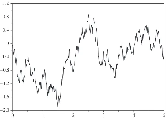
stan-dard Brownian motion. Brownian motion has a fas-cinating history. It is named after the botanist Robert Brown, who first observed, in the 1820s, the irregular motion of pollen grains immersed in water. By the end of the nineteenth century, the phe-nomenon was understood by means of kinetic the-ory as a result of molecular bombardment. Indeed, in 1905, Einstein, although ignorant of the dis-covery of the phenomenon and of previous work on it, predicted its existence from purely theoret-ical considerations. Five years earlier L. Bachelier had employed it to model the stock market, where the analogue of molecular bombardment is the in-terplay of the myriad of individual market decisions that determine the market price.
Standard Brownian motion was rigorously con-structed by N. Wiener in the 1920s as a family of functionals on the space C = C0([0,∞),R) of
real-valued continuous functions on [0,∞) that vanish at zero. In so doing, he equipped the infinite-dimensional space Cwith a Gaussian measure that is now called Wiener measurein his honour. It fol-lows that the paths t→Ba(t)(ω), where ω∈ C, are
continuous. In the 1930s Wiener, together with R. Paley and A. Zygmund, showed that the paths are nowhere differentiable (w.p.1).
Figure 1 presents a simulation of the paths of standard Brownian motion.
Brownian motion with driftis the Lévy process
Ca,b=(Ca,b(t), t≥0), with characteristics (b, a,0) .
Each Ca,b(t) is a Gaussian random variable having
mean vector tb and covariance matrix ta. In fact each Ca,b(t)=bt+Ba(t). A Lévy process has
con-tinuous sample paths (w.p.1), or is Gaussian if and only if it is a Brownian motion with drift.
2. The Poisson Process
A Poisson process Nλ=(Nλ(t), t≥0) with
in-tensity λ >0 is a Lévy process with characteristics (0,0, λδ1), where δ1 is a Dirac mass concentrated
at 1. Nλtakes non-negative integer values, and we
have the Poisson distribution:
P(Nλ(t)=n)=
e−λt(λt)n n! .
The paths of Nλare piecewise constant on each
finite interval, with jumps of size 1 at the random times τn=inf{t≥0, Nλ(t)=n}.
3. The Compound Poisson Process
Let (Yn, n∈N) be a sequence of independent
identically distributed random variables with com-mon law q and let Nλbe an independent Poisson
process. The compound Poisson process is the Lévy processZλ(t)=
Nλ(t)
j=1 Yj. It has characteristic
exponent η(u)=
Rd(eiu·y−1)λq(dy) . The
com-pound Poisson process (with d=1) can be used to model the takings at a till in a supermarket, where
Nλ(t) is the number of customers in the queue at
time t and Yj is the amount paid by the jth
cus-tomer.
4. Interlacing Processes
We can define a Lévy process by the prescrip-tion X(t)=Ca,b(t)+Zλ(t), provided the two
sum-mands are assumed to be independent. We call this an interlacing processsince its paths have the form of continuous motion interlaced with ran-dom jumps of size ||Yn||occurring at the random
times τn(where the Yns are as in Example 3 above). Xhas characteristic exponent
(0.2) η(u)=ib·u−1
2u·au+
Rd(e
iu·y−1)λq(dy),
which is quite close to the general form (0.1). In-deed (0.2) was proposed as the form of the most general ηby the Italian mathematician B. de Finetti in the 1920s. His error was in failing to appreciate that the finite measure λqcan be replaced by a σ -finite Lévy measure ν. But if we do this, (eiu·y−1)
[image:4.594.46.313.44.236.2]may not be ν-integrable and hence we must adjust the integrand. Probabilistically, this corresponds to a lack of convergence of a countable number of “small jumps”, as we will see in the next section. Although (0.2) is incorrect, the most general ηcan be obtained as a pointwise limit of terms of simi-lar type, i.e., η(u)=limn→∞ηn(u) , where each
Figure 1. Simulation of standard Brownian motion. The path is continuous but nowhere differentiable. If you were to zoom in, the fractal nature of the path would become apparent and this reflects the self-similarity of the process.
0 1 2 3 4 5
ηn(u)=i
b−
1 n<||y||<1
yν(dy) ·u −12u·au+
||y||≥1n
(eiu·y−1)λq(dy),
and the integrals must be combined together be-fore the passage to the limit. In the next section we will see the intuition behind this.
From the above examples, the reader may be for-given for thinking that a Lévy process is nothing but the interplay of Gaussian and Poisson measures. In a sense this is correct; however, note that the Gaussian and Poisson measures give rise to ex-treme points of the convex cone of all character-istic exponents. As the following shows, there are some interesting inhabitants of the interior.
5. Stable Lévy Processes
Stable probability distributions arise as the pos-sible weak limits of normalized sums of i.i.d. (i.e., independent, identically distributed) random vari-ables in the central limit theorem. The normal dis-tribution is stable and corresponds to the case in which each of the i.i.d. random variables has finite mean and variance. Stable random variables are those whose laws are stable. They are characterized by the property that if X1and X2are independent
copies of a stable random variable X, then for each c1, c2>0, there exists c >0 and d∈Rdsuch
that cX+d has the same law as c1X1+c2X2. A
Lévy process is stable if each X(t) is stable in this sense. The characteristics of a stable Lévy process are either of the form (b, a,0) (so it is a Brownian motion with drift) or (b,0, ν) , where
ν(dx)= C
|x|α+ddx, with 0< α <2 and C >0. αis
called the index of stability. With the sole exception of the Brownian motions with drift, the random variables of a stable Lévy process all have infinite variance, and if α≤1, they also have infinite mean. One example of interest (in the case d=1) for which α=1 is the Cauchy process, which has the density ft(x)=
t
π(x2+t2). Figure 2 presents a
simulation of its paths in which jump discontinu-ities are represented by vertical lines.
With a little calculus, the characteristic exponent can be transformed to a more useful form. This is particularly simple when X is rotationally invariant, i.e., P(X(t)∈OA)=P(X(t)∈A) , for all
O∈O(d), t≥0, and Borel sets A. We then obtain
η(u)= −σα|u|α, where σ >0. Rotationally
invari-ant stable processes are an importinvari-ant class of self-similar processes, i.e., (X(ct), t≥0) and (cα1X(t), t≥0) have the same finite dimensional
distributions (for each c >0), and this is one reason why such processes are important in applications. Another reason, applying to general stable random variables X, is that they have “heavy
tails”, i.e. P(X > y) behaves asymptotically like y−α
as y→ ∞, as opposed to the exponential decay found in the Gaussian case. Such behavior has been found in models of telecommunications traf-fic on the Internet.
6. Relativistic Processes
1905 was a busy year for Albert Einstein. As well as his work on Brownian motion, mentioned above, he also gave a quantum mechanical explanation of the photoelectric effect (for which he won his Nobel Prize) and developed the special theory of relativ-ity. According to the latter, a particle of rest mass
m moving with momentum phas kinetic energy
E(p)=
m2c4+c2|p|2−mc2, where c is the
ve-locity of light. If we define η(p)= −E(p) , then ηis the characteristic exponent of a Lévy process. We will explore some consequences of this below.
7. Subordinators
A subordinator is a one-dimensional Lévy process (T(t), t≥0) that is nondecreasing (w.p.1). In this case, the Fourier transform that defines the characteristic function can be analytically contin-ued to yield the Laplace transform
E(e−uT(t))=e−tψ(u),for each u >0, where
ψ(u)= −η(iu)=bu+
(0,∞)
(1−e−uy)λ(dy).
Here b≥0 and λis a Lévy measure that satisfies the additional constraints λ(−∞,0)=0 and
(0,∞)(y∧1)λ(dy)<∞.
ψ is called the Laplace exponentof the subor-dinator. The set of all of these is in one-to-one cor-respondence with the set of Bernstein functions for which limx→0f(x)=0 , where we recall that an
[image:5.594.277.547.41.238.2]infinitely differentiable function f on (0,∞) is a Bernstein function if and only if f ≥0 and (−1)nf(n)≤0, for all n∈N.
Figure 2. Simulation of the Cauchy process. The Cauchy process is stable with α= 1. Jump discontinuities are
represented by vertical lines. This process is also self-similar so the path has a fractal nature.
0 1 2 3 4 5
Examples of subordinators include the α-stable ones (0< α <1) that have Laplace exponent
ψ(u)=uα. For the case α=1
2, each T(t) is the first
hitting time of a standard Brownian motion to a level, i.e., T(t)=inf{s >0;B(s)= √t
2}. Furthermore,
each T(t) has a Lévy distribution with density
ft(s)=
t
2√π
s−32e− t2
4s. Another well-known example
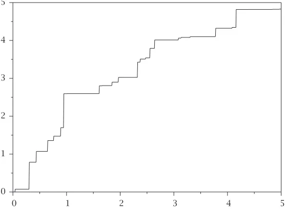
of a subordinator, where each T(t) has a gamma distribution, is depicted in Figure 3.
An important application of subordinators is to the time change of Lévy processes. If Xis a Lévy process with characteristic exponent ηX and T
is an independent subordinator with Laplace exponent λ, then Y(t)=X(T(t)) is a new Lévy process with characteristic exponent ηY = −λ◦ −ηX. This procedure was first investigated by
S. Bochner in the 1950s and is sometimes called “subordination in the sense of Bochner” in his honor. In particular, if X is a Brownian motion (with a a multiple of the identity) and T is an independent α-stable subordinator, then Y is a 2α-stable rotationally invariant Lévy process. 8. The Riemann-Zeta Process
Readers who are interested in number theory may find this example of interest. If ζis the usual Riemann zeta function, we obtain a Lévy process for each u >1 by the following prescription for the characteristic exponent,
ηu(v)=log
ζ(u+iv)
ζ(u) .
This was established by Khintchine in the 1930s.
The Lévy-Itô Decomposition
With the insight we obtained from Example 4, we can now return to the task of trying to understand
the structure of the sample paths of Lévy processes. Given a characteristic exponent, we can always as-sociate to it a Lévy process whose paths are right continuous with left limits (w.p.1). It follows that this process Xcan only have jump discontinuities, and there are, at most, a countable number of these on each closed interval. We formally write
X(t)=Xc(t)+
0≤s≤t∆X(s) , where Xchas
continu-ous paths (w.p.1) and ∆X(s)=X(s)−X(s−) is the “jump” at time s where X(s−)=limu↑sX(u) is the
left limit.
We can describe Xcquite easily. It is a Brownian
motion with drift, Xc(t)=bt+Ba(t) (although this
is by no means easy to prove). The second term is more problematic—in particular, the sum may not converge. It turns out to be helpful to count the jumps up to time tthat are in a given Borel set A
and to introduce
N(t, A)=#{0≤s≤t;∆X(s)∈A}.
Nis a very interesting object—it is in fact a func-tion of three variables—time t, the set A, and the sample point ω. If we fix t and ω, we get a
σ-finite measure on the Borel sets of Rd. On the
other hand, if we fix the set A and ensure that it is bounded away from zero, we get a Poisson process with intensity λ=ν(A) . For these reasons
Nis called a Poisson random measure.
In any finite time, Xcan have only a finite num-ber of jumps of size greater than 1 (or indeed greater than any ǫ >0). We can write this finite sum of jumps as
||x||>1xN(t, dx). Similarly, the sum of
all the jumps of size greater than n1 but less than 1 is
1
n<||x||<1xN(t, dx) ; however, the limit may not
converge as n→ ∞. Paul Lévy argued that the ac-cumulation of a large number of very small jumps may be difficult to distinguish from bursts of de-terministic motion, so one should consider
Mn(t)=
1
n<||x||<1x(N(t, dx)−tν(dx)). (Mn, n∈ N) is a sequence of square-integrable, mean zero mar-tingales and hence is a very pleasant object from both a probabilistic and an analytic viewpoint. In particular the sequence converges in mean square to a martingale M(t)=
0<||x||<1xN˜(t, dx) , where
˜
N(t, dx)=N(t, dx)−tν(dx) is called a compensated Poisson random measure. Lévy’s intuition was made precise by K. Itô, and we can now give the celebrated Lévy-Itô decomposition for the sample paths of a Lévy process:
X(t)=bt+Ba(t)+
|x|<1
xN˜(t, dx)+ (0.3)
|x|≥1
xN(t, dx).
Readers should beware of generalizing from the Gaussian to this more general case. For example,
[image:6.594.41.319.46.251.2]bt is not in general the mean of X(t) —indeed, as we saw in Example 5, this may not exist. The Figure 3. Simulation of the gamma subordinator. In contrast
to the cases shown by the previous two figures, the sample paths of subordinators are considerably more regular. The path is a non-decreasing step function with jump discontinuities again shown as vertical lines.
0 1 2 3 4 5
“martingale part” of X(t) , i.e., the process
M(t)+Ba(t), has moments to all orders, so if X(t)
itself fails to have an nth moment this is entirely due to the influence of “large jumps”.
Applications to Finance
A sociologist investigating the behavior of the prob-ability community during the early 1990s would surely report an interesting phenomenon. Many of the best minds of this (or any other) generation began concentrating their research in the area of mathematical finance. The main reason for this can be summed up in two words—option pricing. Essentially, an option is a contract that confers upon the holder the right, but not the obligation, to purchase (or sell) a unit of a certain stock for a fixed price kon (or perhaps before) a fixed expiry date T, after which the option becomes worthless. For the option to make sense, kshould be consid-erably less than the current price of the stock. If the stock price rises above k, the holder of the op-tion may make a considerable profit; on the other hand, if the stock price falls dramatically, losses will be considerably less through buying options than by purchasing the stock itself.
The key question is—does the market deter-mine a unique price for a given option, and if so, can this price be explicitly computed? Much of the current interest in the subject derives from Nobel-prize winning work of F. Black, M. Scholes and R. Merton in the 1970s who gave a positive answer to this question. Underlying their analysis was a model of stock prices that improved upon that of Bache-lier by using geometric Brownian motion; i.e., the price S(t) of a given stock at time tis
S(t)=S(0) exp
µ−1
2σ
2
t+σ B(t)
.
The constant µ∈Ris the (logarithmic) expected rate of return, while σ >0, called the volatility,is a measure of the excitability of the market. We will have more to say about volatility below. Black and Scholes obtained an exact formula for the unique price of a European option(i.e., one that can only be exercised at time T) using the normal distribu-tion. The derivation of this formula involves the use of tools such as martingales and Girsanov trans-forms, and it is this link with stochastic analysis that so excited the probabilistic community.
Although very elegant, the Black-Scholes-Merton model has limitations and possible defects that have led many probabilists to query it. Indeed, em-pirical studies of stock prices have found evidence of heavy tails, which is incompatible with a Gauss-ian model, and this suggests that it might be fruit-ful to replace Brownian motion with a more gen-eral Lévy process. Indeed, H. Geman, D. Madan and M. Yor have argued that this is quite natural from
the point of view of the Lévy-Itô decomposition (0.3), where the small jumps term
|x|<1xN˜(t, dx)
de-scribes the day-to-day jitter that causes minor fluc-tuations in stock prices, while the big jumps term
|x|≥1xN(t, dx) describes large stock price
move-ments caused by major market upsets arising from, e.g., earthquakes or terrorist atrocities.
If we set aside Brownian motion, there are a plethora of Lévy processes to choose from, and our choice must enable us to derive a pricing formula that market analysts can compute with. One in-teresting group of candidates is the (symmetric) hy-perbolic Lévy processes, whose financial applications have been extensively developed by E. Eberlein and his group in Freiburg, Germany. These are processes with no Brownian motion part in (0.3), and the characteristic function is given by
φt(u)=
ζ K1(ζ)
K1(
ζ2+δ2u2)
ζ2+δ2u2
t
,
where K1is a Bessel function of the third kind, and
ζ and δare non-negative parameters.
Hyperbolic Lévy processes were discovered by O. Barndorff-Nielsen the 1970s and used as mod-els for the distribution of particle size in wind-blown sand deposits. N. H. Bingham and R. Keisel make an interesting analogy between the dynam-ics of sand production and stock prices in that just as large rocks are broken down to smaller and smaller particles “this ‘energy cascade effect’ might be paralleled in the ‘information cascade effect’, whereby price-sensitive information originates in, say, a global newsflash and trickles down through national and local level to smaller and smaller units of the economic and social environment.”
A problem with non-Gaussian option pricing is that the market is “incomplete”, i.e., there may be more than one possible pricing formula. This is clearly undesirable, and a number of selection prin-ciples, such as entropy minimization, have been em-ployed to overcome this problem. For hyperbolic processes, a pricing formula has been developed that has minimum entropy and that is claimed to be an improvement on the Black-Scholes formula. Another problem with the Black-Scholes-Merton formula is the constancy of the volatility. Empirical studies suggest that this should vary to give a curve called the “volatility smile”. This has prompted some authors to propose “stochastic volatility models” wherein σ is replaced in the standard Black-Scholes model by a random process that solves a stochastic differential equation. There are a number of different approaches to this; e.g., O. Barndorff-Nielsen and N. Shephard have recently proposed that (σ(t)2, t≥0) should be an
σ(t)2=e−λtσ(0)2+
t
0
e−λ(t−s)dT(λs),
where λ >0. As Thas finite variation (w.p.1), the integral is well defined in the random Lebesgue-Stieltjes sense.
Readers who want to learn more about “Lévy fi-nance” should consult [12], [4] , chapter 5 of [1], and references therein.
Markov Processes, Semigroups, and Pseudodifferential Operators
Lévy processes are, in particular, Markov processes, i.e., their past and future are independent, given the present. This is formulated precisely using the conditional expectation: E(f(X(t+u))|Ft) = E(f(X(t+u))|X(t)) ,for all t, u≥0 and all f ∈Bb(Rd)—the Banach space, under the
supre-mum norm, of all bounded Borel measurable functions on Rd. Here “the past” F
tis the smallest
sub-σ-algebra of F with respect to which all
X(s)(0≤s≤t) are measurable. We define a two-parameter family of linear contractions (Ts,t; 0≤s≤t <∞) on Bb(Rd) by the prescription
(Ts,tf)(x)=E(f(X(t))|X(s)=x)=
Rdf(x+y)pt(dy) .
Then the Markov property implies that these form an evolution, i.e., Tr ,sTs,t=Tr ,t, for all r≤s≤t.
Note that these operators all commute with the nat-ural action of the translation group of Rdon B
b(Rd).
Lévy processes form a nice subclass of Markov processes. First, they are time-homogeneous, i.e., Ts,t=T0,t−sfor all s≤t. If we now write Tt =T0,t,
the evolution property becomes the semigroup law TsTt=Ts+t. Second, Lévy processes are Feller
processes, i.e., each Ttpreserves the Banach space C0(Rd) of continuous functions on Rdthat vanish
at infinity and limt↓0||Ttf−f|| =0 , for all f ∈C0(Rd). Hence (Tt, t≥0) is a strongly
continu-ous, one-parameter contraction semigroup on
C0(Rd) , and by the general theory of such
semigroups, we can assert the existence of the generator Af =limt↓0
T(t)f−f
t , for all f ∈DA. The
domain DAis a linear space that is dense in C0(Rd)
and Ais a closed linear operator. We can explicitly compute the semigroup and its generator as pseu-dodifferential operators. For convenience, we work in Schwartz space S(Rd) —the space of all smooth
functions on Rdthat are such that they and all their
derivatives decay to zero at infinity faster than any negative power of |x|. S(Rd) is dense in C
0(Rd) and
is a natural domain for the Fourier transform ˆ
f(u)=(2π)−d2
Rde−i(u,x)f(x)dx. Fourier inversion
then yields f(x)=(2π)−d2
Rdfˆ(u)ei(u,x)du.Applying
theorem 0.1, we compute (Ttf)(x)=(2π)−
d 2
Rde
i(u,x)etη(u)fˆ(u)du,
so that Tt is a pseudodifferential operator with
symbol etη. Formal differentiation can be justified,
and we find that (Af)(x)=(2π)−d2
Rde
i(u,x)η(u)ˆf(u)du,
so Ais also a pseudodifferential operator, with sym-bol η. Using the Lévy-Khintchine formula (0.1) and elementary properties of the Fourier transform, we obtain the following explicit form for the action of the generator on S(Rd)
(Af)(x)=
d
i=1
bi∂if(x)+
1 2
d
i,j=1
aij∂i∂jf(x)
(0.4)
+
Rd−{0}
f(x+y)−f(x)−
d
i=1
yi∂if(x)1||y||<1(y)
ν(dy).
Using more sophisticated methods the domain in (0.4) can be extended to a larger space of twice dif-ferentiable functions in C0(Rd). Here are some
spe-cific examples of interesting generators:
1. Brownian motion (with a=I) is generated by (one-half times) the Laplacian, i.e.,
A=12d
i=1∂2i = 12∆.
2. Rotationally invariant α-stable processes (with
σ=1) are generated by fractional powers of the Laplacian: A= −(−∆)α2.
3. For the relativistic process, we have
A= −(√m2c4−c2∆−mc2).
In the last example, −A is called a relativistic Schrödinger operatorin quantum theory. Note that
Ais obtained from its symbol through the corre-spondence p↔ −i∇, which is precisely the usual rule for quantization, although this is more natu-rally carried out in a Hilbert space setting (see below).
If AZ is the generator of the Lévy
process Z(t)=X(T(t)) obtained from a Lévy processXwith characteristic exponent ηX,
associ-ated semigroup (TX
t , t≥0), and generator AXusing
an independent subordinator T with Laplace ex-ponent ψ, then the identity ηZ= −ψ◦ −ηX,
quan-tizes nicely to yield AZ= −ψ(−AX) . In particular,
we can use the α-stable subordinators to define fractional powers of −AXusing the following
beau-tiful formula
−(−AX)αf = α
Γ(1−α)
(0,∞)
(TX s f−f)
ds s1+α.
A deep generalization due to R. S. Phillips allows the replacement of AXand TtXwith the generator
of a general contraction semigroup on a Banach space.
The semigroup associated with each Lévy process also operates in each Lp(Rd)(1≤p <∞)
Since S(Rd) is dense in each Lp(Rd), the
pseudo-differential operator representations discussed above still hold here. From now on, we take p=2. The generator corresponding to the symbol η
has maximal domain Hη(Rd)—the nonisotropic
Sobolev space of all f ∈L2(Rd) for which
Rd|η(u)|2|fˆ(u)|2du <∞.
Standard semigroup theory tells us that a nec-essary and sufficient condition for each Ttto be
self-adjoint is that −Ais positive, self-adjoint. A nec-essary and sufficient condition for this is that the associated Lévy process is symmetric, i.e.,
P(X(t)∈A)=P(X(t)∈ −A) , and this holds if and only if
η(u)= −1
2u·au+
Rd−{0}(cos(u·y)−1)ν(dy).
This yields a probabilistic proof of self-adjoint-ness (on Hη(Rd)) of each of the three operators
dis-cussed above.
Let A be the self-adjoint generator of a sym-metric Lévy process and for each f , g∈C∞
c (Rd),
define E(f , g)= −< f , Ag >, then E extends to a
symmetric Dirichlet form in L2(Rd) , i.e., a closed
symmetric form in H with domain D, such that
f ∈D⇒(f∨0)∧1∈D and E((f∨0)∧1)≤ E(f) for all f ∈D, where we have written E(f)= E(f , f) . A straightforward calculation yields
E(f , g) = 1 2
d
i,j=1
aij
Rd(∂if)(x)(∂jg)(x)dx + 12
(Rd×Rd)−D(f(x)−f(x+y))·
(g(x)−g(x+y))ν(dy)dx,
where Dis the diagonal, D= {(x, x), x∈Rd}. This
is the prototype for the Beurling-Deny formulafor symmetric Dirichlet forms.
Now we return to the space C0(Rd). The ideas we
explored there have a far-reaching generalization, originally due to W. von Waldenfels and P. Cour-rège in the early 1960s and recently systematically explored by N. Jacob and his school in Erlangen and Swansea [7]. The main starting point of this is that if Xis a general Feller process defined on Rdthat
has the property that the smooth functions of com-pact support are contained in the domain of its gen-erator A, then we can always represent A as a pseudodifferential operator
(Af)(x)=(2π)−d2
Rde
i(u,x)η(x, u)ˆf(u)du.
Note that the symbol η now has an additional x -dependence; however, each η(x,·) is still a char-acteristic exponent, so that we get an appealing in-tuitive understanding of X as a “field of Lévy processes” indexed by space. Aficionados of
pseu-dodifferential operators should be aware that the map x→η(x, u) does not, in general, have nice smoothness properties.
Recurrence, Transience, and Bound States
From an intuitive point of view a stochastic process is recurrentat a point x if it visits any arbitrarily small neighborhood of that point an infinite num-ber of times (w.p.1), and it is transientif each such neighborhood is only visited finitely many times (w.p.1). More precisely, a Lévy process is recurrent (at the origin) if lim inft→∞|X(t)| =0 (w.p.1) and
transient (at the origin) if limt→∞|X(t)| = ∞(w.p.1).
The recurrence/transience dichotomy holds in that every Lévy process is either recurrent or transient. In the 1960s, S. C. Port and C. J. Stone proved that a Lévy process is recurrent if and only if
||u||<aℜ
1
−η(u)
du= ∞for any a >0. It follows that Brownian motion is recurrent for d=1,2 and that for d=1 every α-stable process is recurrent if 1≤α <2 and transient if 0< α <1 . For d≥3, every Lévy process is transient.
In the 1990s, R. Carmona, W. C. Masters, and B. Simon studied the spectral properties of Hamil-tonian operators acting in L2(Rd) of the form H=H0+V, where H0 is (minus) the generator of
a symmetric Lévy processXand Vis a suitable po-tential. In particular, they were able to show that
H has at least one bound state (i.e., a negative eigenvalue) if and only if Xis recurrent. In partic-ular, in the physically interesting case in which H0
is a relativistic Schrödinger operator, bound states are obtained only in dimension 1 and 2.
Lévy Processes in Groups
So far we have dealt exclusively with Lévy processes taking values in a Euclidean space. Now we will re-place Rdwith a topological group G. First some
gen-eral remarks. The interaction between probability theory and groups has been an active area of re-search since the 1960s—indeed, this is the natural setting for studying the interaction of “chance” with “symmetry”. One area of research that is cur-rently attracting enormous interest is random ma-trix theory [5], partly because of intriguing links be-tween the asymptotics of uniformly distributed matrices in the unitary group U(n) and the zeros of the Riemann zeta function. A survey on random walks and invariant diffusions in groups can be found in [10], with particular emphasis on the re-lationship between the asymptotic behavior of the process and the volume growth of the group.
A Lévy process on a topological group Gis de-fined exactly as in the Euclidean case, but within the axioms (L1) and (L3), the increment X(t)−X(s) is replaced by X(s)−1X(t) (with the group operation
written multiplicatively), whereas in (L2), the role of 0 is played by the neutral element that we de-note by e. If pt is the law of X(t) , then (pt, t≥0) is
probability measures on G, so that in particular
ps+t(A)=
Gpt(τ−1A)ps(dτ) .
There are three cases of interest—locally com-pact abelian groups (LCA groups), Lie groups, and general locally compact groups. The LCA case was extensively studied during the 1960s. The fact that the dual group ˆG of characters is itself an LCA group allows a natural generalization of the Fourier transform from Rdto G, and a Lévy-Khintchine
for-mula that characterizes Lévy processes can hence be developed similarly to the Euclidean case. We will not dwell further on this topic here; interested readers are directed to section 5.6 in [6].
The case in which Gis a Lie group has been ex-tensively studied. For non-abelian G, there is no di-rect analogue of the Fourier transform available, and one of the joys of the subject is the challenge of surmounting this obstacle using tools from semigroup theory, stochastic analysis, group rep-resentations, and noncommutative harmonic analy-sis. The first important step in this direction was taken by G. A. Hunt in 1956. He effectively char-acterized Lévy processes in Lie groups by gener-alizing the formula (0.4) for the generator in Rd. To
be precise, let X=(X(t), t≥0) be a Lévy process on a d-dimensional Lie group Gand let ptbe the law
of each X(t) . We obtain a one-parameter, strongly continuous, contraction semigroup (Tt, t≥0) with
generator Aon C0(G) by the prescription
(Ttf)(τ)=E(f(τX(t)))=
G
f(τσ)pt(dσ).
Note that Ttcommutes with left translations. Now
let {Y1, . . . , Yd}be a fixed basis for the Lie algebra g of left-invariant vector fields on G. Define a linear manifold C2(G) that is dense in C0(G) by the
prescription C2(G)= {f ∈C0(G);Yif ∈C0(G) and
YiYjf ∈C0(G) for all 1≤i, j≤n}. Hunt showed
that there exist functions xi∈C2(G),1≤i≤n
so that (x1, . . . , xn) is a system of canonical
coordinates for G at e. A Lévy measure ν is a Borel measure on G− {e} for which
G−{e}
d
i=1xi(σ)2
∧1ν(dσ)<∞. Hunt was then able to obtain the following key result:
Theorem 0.2 [Hunt’s Theorem]. If X is a Lévy process in Gwith infinitesimal generator A,then
1.C2(G)⊆Dom(A).
2. For each τ∈G, f ∈C2(G),
(Af)(τ)=
d
i=1
biYif(τ)+1
2
d
i,j=1
aijYiYjf(τ)
(0.5)
+
G−{e}
f(τσ)−f(τ)−
d
i=1
xi(σ)Yif(τ)
ν(dσ),
where b=(b1, . . . , bn)∈Rn, a=(a
ij), is a
non-negative definite, symmetric n×nreal-valued ma-trix and νis a Lévy measure on G− {e}.
Conversely, any linear operator with a representa-tion as in (0.5) is the restricrepresenta-tion to C2(G)of the
in-finitesimal generator of some Lévy process.
The characteristics (b, a, ν) of a Lévy process de-termine its law, just as in the Euclidean case.
In the 1990s, H. Kunita and the author were able to generalize the Lévy-Itô decomposition to the extent that for each f ∈C2(G) , the real-valued
process f(X)=(f(X(t), t≥0) can be described (using stochastic integrals in the sense of K. Itô) in terms of a Brownian motion on Rdand a Poisson
random measure on R+×(G− {e}). We now give some examples of Lévy processes on a Lie group
G:
1. Brownian motion in G.
This is a Lévy process that has characteristics (0, I,0) . It has continuous sample paths (w.p.1), and its generator is (up to the usual factor of one-half) a left-invariant Laplacian on G, ∆G=
d
i=1Yj2.
The basis dependence is a nuisance here. It can be dispensed with by equipping Gwith a left-invari-ant Riemannian metric m, with respect to which
{Y1, . . . , Yd}is orthonormal. ∆Gis then the
Laplace-Beltrami operator associated to (G, m) and the cor-responding Brownian motion is a geometrically in-trinsic object—indeed, it has played a central role in recent years within the development of analy-sis in path and loop spaces.
2. The Compound Poisson Process
Let (γn, n∈N) be a sequence of i.i.d. random
variables taking values in G with common law µ
and let (N(t), t≥0) be an independent Poisson process with intensity λ >0. We define the com-pound Poisson process in Gby Y(t)=γ1γ2. . . γN(t).
In this case the generator is bounded and is given by (Af)(τ)=
G(f(τσ)−f(τ))ν(dσ), for each f ∈C0(G) where the Lévy measure ν(·)=λµ(·) is
finite.
3. Stable Processes
The theory of stable processes in Lie groups was developed by H. Kunita in the 1990s. His ap-proach was to generalize the self-similarity prop-erty, and for this he needed a notion of scaling. This is provided by a dilation, i.e., a family of automor-phisms δ=(δ(r), r >0) for which δ(r)δ(s)=δ(r s) for all r , s >0, which also possess suitable conti-nuity properties. A Lévy processX in G is stable
in such groups have some surprising properties, e.g., Kunita has shown that there is no dilation with respect to which Brownian motion in the Heisenberg group is stable. It is however possible to construct a stable process on this group whose first two components are Brownian motion whereas the third is a Cauchy process.
4. Subordinated Processes
Let Y=(Y(t), t≥0) be a Lévy process on Gand
T=(T(t), t≥0) be a subordinator that is inde-pendent of Y. Just as in the Euclidean case, we can construct a new Lévy process Z=(Z(t), t≥0) by the prescription Z(t)=Y(T(t)) , for each t≥0.
Lévy processes in Lie groups is a subject that is currently undergoing intense development—see the author’s survey article in [2] and the recent book by M. Liao [8]. The latter contains a lot of interest-ing material on the asymptotics of Lévy processes on noncompact semisimple Lie groups, as t→ ∞. Liao has also found some classes of Lévy processes on compact Lie groups that have L2
-densities. The density then has a “noncommutative Fourier series” expansion via the Peter-Weyl theo-rem. In the special case of Brownian motion on
SU(2), Liao obtains the following beautiful formula for its density ρt at time t:
ρt(θ)=
∞
n=1
nexp
−(n642−π1)2t sin(2sin(2π nθπ θ)),
where θ∈(0,1] parameterizes the maximal torus
{diag
e2π iθ, e−2π iθ
, θ∈[0,1)}.
Another important theme, originally due to R. Gangolli in the 1960s, is to study spherically sym-metric Lévy processeson semisimple Lie groups G
(i.e., those whose laws are bi-invariant under the action of a fixed compact subgroup K). Using Har-ish-Chandra’s theory of spherical functions, one can carry out “Fourier analysis” and obtain a Lévy-Khintchine-type formula. One of the reasons why this is interesting is that G/K is a Riemannian (globally) symmetric space and all such spaces can be obtained in this way. The Lévy process in G pro-jects to a Lévy process in G/K, and this is the pro-totype for constructions of Lévy processes in more general Riemannian manifolds.
Before leaving the subject of Lévy processes in groups, we briefly mention the general locally com-pact case. Work on Hilbert’s fifth problem during the 1950s established that every such group has an open subgroup of the identity that is a projec-tive limit of Lie groups. This enables the use of Lie group methods within the more general case, and there has been intensive work on this subject since the 1970s by the German school of H. Heyer, W. Hazod, E. Siebert, and their students ([6]). Quite re-cently, the path properties of Brownian motion in general locally compact groups have been
investi-gated by A. Bendikov and L. Saloff-Coste at Cornell. It will be interesting to see if the new techniques they’ve developed can be applied to more general classes of Lévy processes.
Lévy Processes in Quantum Groups
Through the work of physicists such as N. Bohr, M. Born, and W. Heisenberg and its mathematical formulation by J. von Neumann, we came to a dual understanding of quantum mechanics. On the one hand, physical observables such as position, mo-mentum, energy, and spin should be described as (not necessarily bounded) self-adjoint linear oper-ators acting in a complex Hilbert space. On the other hand, these observables are also random quantities whose statistical properties are deter-mined by a unit vector in Hilbert space (for pure states) or a more general density matrix (for mixed states). However, the celebrated Heisenberg un-certainty principle tells us that certain pairs of these operators, such as those representing posi-tion and momentum, fail to commute. Conse-quently they cannot both be described together as measurable functions on the same probability space using Kolmogorov’s prescription, and hence they cannot have a joint probability distribution.
To describe the probabilistic features of quan-tum theoretic phenomena systematically, we need to take an algebraic viewpoint. We define a quan-tum probability spaceto be a pair (B, ω) where B
is a complex ∗-algebra (with identity I) and ωis a state on B, i.e., a positive, linear map for which
ω(I)=1. If B is a C∗-algebra, we can recover a
Hilbert space viewpoint by taking the Gelfand-Naimark-Segal representation.
Quantum stochastic processes were introduced by L. Accardi, A. Frigerio, and J. T. Lewis in the 1980s. Every “classical” stochastic process (X(t), t≥0) with state space Egives rise to a fam-ily of ∗-homomorphisms (jt, t≥0) from the ∗-algebra Bb(E) of bounded measurable functions
on E into the ∗-algebra L∞(Ω,F, P) by the
pre-scription jt(f)=f◦X(t) . Given a quantum
proba-bility space (B, ω) and a ∗-algebra A, a quantum stochastic process is a family (jt, t≥0) of ∗-homomorphisms from Ainto B. Many concrete examples of these have been constructed using the quantum stochastic calculus of R. L. Hudson and K. R. Parthasarathy as solutions of operator-valued stochastic differential equations driven by “quantum noise”, i.e., the creation, conservation, and annihilation processes acting in a suitable Fock space.
In order to clarify the last remark, we make a brief diversion. Fock space Γ(h) over a complex Hilbert space h is Γ(h) :=∞
n=0h(n), where
h(0)=C, h(1)=h, and h(n)is the tensor product of
space, which are the closed subspaces obtained by restricting to symmetric or antisymmetric tensors, respectively. For each f ∈hthe creation operator
a†(f) maps each h(n)to h(n+1)while the annihilation
operator a(f) maps each h(n)to h(n−1). For each
self-adjoint T acting in h, the conservation operator
dΓ(T) maps h(n)to itself. All three types of
opera-tor are densely defined linear operaopera-tors in Γ(h) (see, e.g., [9] for precise definitions). As a by-product of work on factorizable representations of current groups in the 1960s and 1970s it was found that any Lévy processX=(X(t), t≥0) on Rdcan
be realized as a family of self-adjoint operators act-ing in a symmetric Fock space, where the Lévy-Itô decomposition (0.3) appears as a certain combi-nation of creation, conservation, and annihilation operators. In the 1980s, Hudson and Parthasarathy realized that they could build interesting classes of quantum stochastic processes by developing a stochastic calculus in which each of the creation, conservation, and annihilation parts is treated as a separate operator-valued process rather than in a special “classical” self-adjoint combination.
We can now make an attempt at defining a “quantum Lévy process”. At the very least this should be a quantum stochastic process (jt, t≥0)
where each jt is embedded as k0,tinto an
associ-ated two-parameter family of ∗-homomorphisms (ks,t,0≤s≤t <∞) which are the “increments” of
the process. We generalize the key axiom (L1). The stationary increments requirement becomes
ω(ks,t(a))=ω(k0,t−s(a)), for each a∈A. For
inde-pendent increments, we have a choice from a num-ber of competing algebraic notions of indepen-dence, each of which will yield a distinct notion of Lévy process. The simplest, called tensor(or bosonic) independence, requires that
ω(ks1,t1(a1)ks2,t2(a2)· · ·ksn,tn(an))= n
i=1
ω(ksi,ti(ai)),
for all n∈N, a1, . . . , an∈A,0 ≤ s1 ≤ t1 ≤ s2 ≤
t2· · · ≤ sn ≤ tn<∞, whenever each pair ksi,ti(ai)
and ksj,tj(aj) commute. Other notions of
indepen-dence that could be used include the fermionic (or
Z2 graded version) or the free independence of
D. Voiculescu. Axioms (L2) and (L3) translate rather easily into this framework; however, the concept we have thus obtained is too general, as it is not clear how ks,t has captured the notion of
“incre-ment”.
To overcome this problem, we need to general-ize the group concept algebraically, and this is cisely the purpose of quantum groups. More pre-cisely, we need A to be a ∗-bialgebra, i.e., a
∗-algebra in which the multiplication and identity have been dualized to give a compatible co-algebra structure. We thus require that there are two ∗-homomorphisms, a comultiplication
∆:A→A⊗Aand a co-unit ε:A→Cwhich satisfy the co-associativity and co-unit axioms:
(id⊗∆)◦∆=(∆⊗id)◦∆,
(id⊗ε)◦∆=(ε⊗id)◦∆,
where id is the identity mapping.
If Ais a ∗-bialgebra, we obtain a quantum Lévy process on Awhen we augment the generalizations of (L1) to (L3) with an additional axiom
(L0)kr ,s∗ks,t=kr ,t, for all 0≤r ≤s≤t <∞,
where the convolutionis given by
kr ,s∗ks,t=mB◦(kr ,s⊗ks,t)◦∆;
here mBdenotes the multiplication in B.
To understand the meaning of (L0) in the sim-plest possible context, let Xbe a Lévy process in a finite group G, and take Ato be the ∗-bialgebra of all complex valued functions on G with the usual pointwise algebra operations and comultiplication (∆f)(σ1, σ2)=f(σ1σ2) and co-unit ε(f)=f(e) . Take
B=L∞(Ω,F, P) and each k
s,tf =f◦X(s)−1X(t) .
Then (L0) precisely expresses the “increment prop-erty”, X(r)−1X(s)X(s)−1X(t)=X(r)−1X(t) .
Quantum Lévy processes first arose in work by W. von Waldenfels on a model of the emission and absorption of light by atoms interacting with “noise”. The quantum stochastic process obtained appeared to be a noncommutative analogue of a Lévy process on the unitary group U(d), and this was made precise in terms of quantum Lévy processes when U(d) was replaced by a noncom-mutative ∗-bialgebra that generalizes the coeffi-cient algebra of U(d). The theory of quantum Lévy processes has been extensively developed by M. Schürmann and U. Franz in Greifswald, Ger-many (see [13] or Chapter 7 of [9]). In particular, all quantum Lévy processes are equivalent to so-lutions of quantum stochastic differential equations driven by creation, conservation, and annihilation processes acting in a suitable Fock space.
We briefly describe one interesting application of quantum Lévy processes to classical probability. Let B=(B(t), t≥0) be a one-dimensional Brownian motion and g(t)=sup{0≤s≤t;B(s)=0}. Azéma’s martingale M(t)=π2sign(B(t))
t−g(t) is a martingale with respect to the filtration Ft= σ{M(s); 0≤s≤t}. This process has many intrigu-ing features, e.g., M. Emery proved that it shares with Brownian motion and the compensated Poisson process the rare property of being “chaotically com-plete” (i.e., the linear span of all multiple Wiener in-tegrals is dense in the natural L2space), but it is not