This is a repository copy of A Parameterised Complexity Analysis of Bi-level Optimisation
with Evolutionary Algorithms.
White Rose Research Online URL for this paper:
http://eprints.whiterose.ac.uk/120163/
Version: Submitted Version
Article:
Corus, D., Lehre, P.K., Neumann, F. et al. (1 more author) (2016) A Parameterised
Complexity Analysis of Bi-level Optimisation with Evolutionary Algorithms. Evolutionary
Computation, 24 (1). pp. 183-203. ISSN 1063-6560
https://doi.org/10.1162/EVCO_a_00147
[email protected] Reuse
Unless indicated otherwise, fulltext items are protected by copyright with all rights reserved. The copyright exception in section 29 of the Copyright, Designs and Patents Act 1988 allows the making of a single copy solely for the purpose of non-commercial research or private study within the limits of fair dealing. The publisher or other rights-holder may allow further reproduction and re-use of this version - refer to the White Rose Research Online record for this item. Where records identify the publisher as the copyright holder, users can verify any specific terms of use on the publisher’s website.
Takedown
If you consider content in White Rose Research Online to be in breach of UK law, please notify us by
A Parameterized Complexity Analysis of
Bi-level Optimisation with Evolutionary
Algorithms
Dogan Corus
[email protected]
School of Computer Science
The University of Nottingham, UK
Per Kristian Lehre
[email protected]
School of Computer Science
The University of Nottingham, UK
Frank Neumann
[email protected]
Optimisation and Logistics
School of Computer Science
The University of Adelaide, Australia
Mojgan Pourhassan
[email protected]
Optimisation and Logistics
School of Computer Science
The University of Adelaide, Australia
January 10, 2014
Abstract
Bi-level optimisation problems have gained increasing interest in the field of combinatorial optimisation in recent years. With this paper, we start the runtime analysis of evolutionary algorithms for bi-level optimisa-tion problems. We examine two NP-hard problems, the generalised mini-mum spanning tree problem (GMST), and the generalised travelling sales-man problem (GTSP) in the context of parameterised complexity.
For the generalised minimum spanning tree problem, we analyse the two approaches presented by Hu and Raidl (2012) with respect to the num-ber of clusters that distinguish each other by the chosen representation of
possible solutions. Our results show that a (1+1) EA working with the spanning nodes representation is not a fixed-parameter evolutionary algo-rithm for the problem, whereas the global structure representation enables to solve the problem in fixed-parameter time. We present hard instances for each approach and show that the two approaches are highly complemen-tary by proving that they solve each other’s hard instances very efficiently. For the generalised travelling salesman problem, we analyse the prob-lem with respect to the number of clusters in the probprob-lem instance. Our results show that a (1+1) EA working with the global structure representa-tion is a fixed-parameter evolurepresenta-tionary algorithm for the problem.
1
Introduction
Many interesting combinatorial optimisation problems are hard to solve and meta-heuristic approaches such as local search, simulated annealing, evolu-tionary algorithms, and ant colony optimisation have been used for a wide range of these problems.
In recent years, researchers became very interested in bi-level optimisation for single-objective (Koh, 2007; Legillon et al., 2012) and multi-objective prob-lems (Deb and Sinha, 2009, 2010). Such probprob-lems can be split up into an upper and a lower level problem which depend on each other. By fixing a possible solution for the upper level problem, the lower level is optimised with respect to the given objective and the constraints imposed by the choice of the upper level.
Recently, Hu and Raidl (Hu and Raidl, 2011, 2012) have proposed two dif-ferent approaches for the generalised minimum spanning tree problem (GM-STP). Both approaches work with an upper layer and a lower layer solution. The upper layer solutionxis evolved by an evolutionary algorithm whereas the optimal solutiony of the lower layer problem corresponding to a partic-ular search pointxof the upper layer can be found in polynomial time using deterministic algorithms.
Our goal is to understand the two different approaches by parameterised computational complexity analysis (Downey and Fellows, 1999). The compu-tational complexity analysis of meta-heuristics plays a major role in the theoret-ical analysis of this type of algorithms and studies the runtime behaviour with respect to the size of the given input. We refer the reader to (Auger and Doerr, 2011; Neumann and Witt, 2010) for a comprehensive presentation. Parame-terised complexity analysis takes into account the runtime of algorithms in de-pendence of an additional parameter which measures the hardness of a given instance. This allows us to understand which parameters of a given NP-hard optimization problem make it hard or easy to be optimised by heuristic search methods. In the context of evolutionary algorithms, the term fixed-parameter evolutionary algorithms has been defined in (Kratsch and Neumann, 2013). An evolutionary algorithm is called a fixed-parameter evolutionary algorithm for a given parameterkiff its expected runtime is bounded byf(k)·poly(n)where
complex-ity analysis of evolutionary algorithms have been carried out for the vertex cover problem (Kratsch and Neumann, 2013), the computation of maximum leaf spanning trees (Kratsch et al., 2010), makespan scheduling (Sutton and Neumann, 2012b), and the travelling salesperson problem (Sutton and Neu-mann, 2012a).
We push forward the parameterised analysis of evolutionary algorithms and present the first analysis in the context of bi-level optimization. In our investigations, we take into account the two NP-hard problems the gener-alised minimum spanning tree problem (GMSTP) and the genergener-alised travel-ling salesman problem (GTSP) which share the parameter, number of clusters
m. We consider two different bi-level representations for GMTSP which both have a polynomially solvable lower level part. For theSpanning Nodes Repre-sentation, we present worst case examples which show that there are instances leading to an optimization time ofΩ(nm). For theGlobal Structure
Representa-tion, we show that it leads to a fixed-parameter evolutionary algorithm with respect to the number of clustersm. Furthermore, we present an instance class where the algorithm using theGlobal Structure Representationencounters an op-timization time ofmΩ(m). Analysing both approaches on each others
worst-case instances, we show that they solve them very efficiently. This shows the complementary abilities of these two representations for the GMSTP. Then we extend our results forGlobal Structure Representation to GTSP to show that a similar algorithm has an expected optimisation time ofmΩ(m)for this problem as well.
The paper is divided into two main parts according to the two different problems. The first part (based on the conference version (Corus et al., 2013)) where the GMSTP problem is investigated is presented in Section 2. We show hard instances for theSpanning Nodes Representationin Section 2.2 and show that a simple evolutionary algorithms needs exponential time even if the num-ber of clusters is small. In Section 2.3, we examine theGlobal Structure Repre-sentationand show that this leads to fixed-parameter evolutionary algorithms for GMSTP. We point out complementary abilities in Section 2.4. This arti-cle extends the conference version (Corus et al., 2013) by investigations of the GTSP and some generalizations. We examine the GTSP problem with the cor-respondingGlobal Structure Representationin Section 3 and provide upper and lower bounds on the optimisation time of the considered algorithm. Further-more, we point out in Section 4 general characteristics which allows this fixed-parameter result to be extended to other problems.
2
Generalised Minimum Spanning Tree Problem
2.1
Preliminaries
We consider the generalised minimum spanning tree problem (GMSTP) intro-duced in (Myung et al., 1995). The input is given by an undirected complete graphG= (V, E, c)onnnodes with a cost functionc: E → R+ that assigns positive costs to the edges. Furthermore, a partitioning of the node setV into
mpairwise disjoint clustersV1, V2, . . . , Vmis given such thatn=Pmi=1|Vi|. A solution to the GMSTP problem consists of two components, them cho-sen nodesP, calledthe spanning nodes, in themclusters, and a minimum span-ning tree T on the graph induced by the spanned nodes. More precisely, a solution S = (P, T) consists of a node setP = (p1, . . . , pm) ∈ Vm, where
Vm=V
1×V2× · · · ×Vmand a spanning treeT ⊆Eon the subgraphG[P] =
G(P,{e∈E|e⊆P})induced byP. The cost ofTis the cost of the edges inT, i. e.,
C(T) = X
(u,v)∈T
c(u, v).
The goal is to compute a solutionS∗ = (P∗, T∗)which has minimal cost
among all possible solutionsS= (P, T). For an easier presentation, we assume in some cases that edge costs can be∞. In this case, we restrict our investi-gations to solutions that do not include edges with cost∞. Alternatively, one might view this as the GMSTP defined on a graph that is not necessarily com-plete.
The GMSTP problem is NP-hard (Myung et al., 1995) and two different bi-level evolutionary approaches have been examined in (Hu and Raidl, 2012). The first approach presented in (Hu and Raidl, 2012) uses theSpanned Nodes Representation. It selects in the upper level problem a node for each cluster and computes on the lower level a minimum spanning tree (using for example Kruskal’s algorithm in timeO(mlogm)) on the induced subgraph.
The second approach uses theGlobal Structure Representation. It constructs a complete graphH = (V′, E′)from the given input graphG= (V, E, c)and the
set of pair-wise disjoint clustersV1, V2, . . . , Vm. The nodevi ∈V′,1 ≤i≤m, corresponds to the clusterViinG. The search space for the upper level consists of all spanning trees ofH and the spanned nodes of the different clusters are selected in timeO(n2)using the dynamic programming approach of Pop (Pop,
2004).
For our theoretical investigations, we measure the runtime of the algo-rithms by the number of fitness evaluations required to obtain an optimal solu-tion. We call this theoptimization timeof the examined algorithm. Theexpected optimization timerefers to the expected number of fitness evaluations until an optimal solution has been obtained for the first time.
2.2
Spanned Nodes Representation
al-gorithm that runs in timeO(ng(m))whereg(m)is a computable function only
depending onm, when choosing the number of clustersmas a parameter.
Theorem 1. For any instance of the GMSTP problem, the expected time until the cluster based (1+1) EA reaches the optimal solution isO(nm).
Proof. For any search point x, let w(x) ∈ [m]denote the number of clusters where the spanned node representation includes a suboptimal node. If the algorithm chooses all w(x) suboptimal clusters for mutation and selects the optimal node in each of them, then the optimal solution is obtained. Since
w(x)≤m, the probability that all suboptimal clusters are mutated in a single step is at least(1/m)m. The probability of choosing the optimal node in cluster
iis1/|Vi|. Thus, the probability of jumping to the optimal solution from any search point is at least
(m)−m m
Y
i=1
|Vi|−1.
SincePm
i=1Vi=n, it holds that m
Y
i=1
1
|Vi| ≥(m/n) m.
Therefore, the probability of reaching the optimal solution in one step isΩ(n−m), and the expected time to reach the optimal solution is bounded from above by
O(nm).
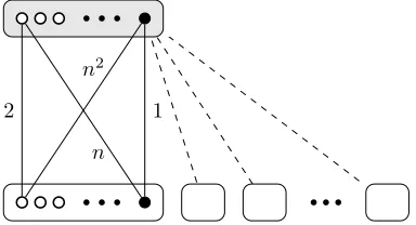
We now consider an instance of GMSTP which is difficult for the cluster based (1+1) EA. The hard instanceGS for theSpanning Nodes Representationis illustrated in Figure 1. It consists ofmclusters, where one cluster is called the
centralcluster, and them−1other clusters are calledperipheralclusters. Each cluster containsn/mnodes and we assume that n = m2 holds. The nodes
in the peripheral clusters are called peripheral nodes, and the nodes in the central cluster are called central nodes. Within each cluster, one of the nodes is calledoptimal, and is marked black in the figure. The remaining(n/m)−1
nodes are calledsub-optimalnodes, and are marked white in the figure. The instance is a bi-partite graph, where edges connect peripheral nodes to central nodes. The cost of any edge between two optimal nodes is 1, the cost of any edge between two suboptimal nodes is 2. The cost of any edge between a suboptimal peripheral node and the optimal central node isn2, and the cost of
any edge between an optimal peripheral node and a suboptimal central node is
n. A cluster is calledoptimalin a solution, if the solution has chosen the optimal node in that cluster.
Theorem 2. Starting with an initial solution chosen uniformly at random, the ex-pected optimization time of the cluster based (1+1) EA onGSisΩ(nm).
1
n n2
[image:7.612.212.404.125.229.2]2
Figure 1: Hard instanceGSforSpanning Node Representation.
Proof. We define two phases for the run of the (1+1) EA. The first phase consists of the firstn−1iterations while the second phase starts at the end of the first phase and continues fornm/12iterations. Four distinct events are considered
failures during the run of the (1+1) EA for the instance described above.
1. The first failure occurs if during the first phase of the run, the algorithm obtains a search point with less thanm/6sub-optimal peripheral clusters.
2. The second type of failure occurs when the central cluster fails to switch to a suboptimal node at least once during the first phase.
3. The third type of failureoccurs when the algorithm does not switch all the optimal peripheral clusters to suboptimal clusters during the second phase.
4. The fourth failure corresponds to a direct jump to the optimal solution during the second phase.
We first show that the probability of the first failure event is at mostexp(−m
12).
This implies that with overwhelmingly high probability, a constant fraction of peripheral clusters is always suboptimal during the firstn−1iterations. For
i∈[m−1]andt≥0, letZi(t),be a random variable such thatZi(t) = 1if cluster
Viis always sub-optimal in iteration 0 through iterationt, andZi(t) = 0 other-wise. The probability that a suboptimal node is selected in the initial solution is1−m/n. In the following iterations, the probability that a cluster is selected for mutation and that its new spanned node is optimal is(1/m)(m/n) = 1/n. So it is clear that
Pr (Zi(t) = 1)≥(1−m/n)(1−1/n)t.
By linearity of expectation,
E
"m−1
X
i=1
Zi(t)
#
≥(m−1)1−m
n
1−1
n
t
Considering a phase length oft = n−1, and assuming thatmis sufficiently large andn=m2holds, we get
E
"m−1
X
i=1
Zi(t)
#
≥ m3 .
Finally, a Chernoff bound (Motwani and Raghavan, 1995) implies that
Pr m−1
X
i=1
Zi(t)≤
1−12
m
3
!
≤exp (−m/12).
We then show that the probability of the second failure event isexp(−Ω(√n)). In each iteration the probability to switch the central cluster to a suboptimal node is at least
p= 1
m
1−m
n = Ω 1 √ n .
The probability that this event does not occur inn−1steps is
(1−p)n−1=(1
−p)1/p(n
−1)p
≤exp(−p(n−1)) = exp(−Ω(√n)).
Now, we show that the probability of the third failure event is less than
n−m/12, assuming that the first two failure events do not occur. As long as the
central cluster remains suboptimal, switching a suboptimal node in a periph-eral cluster to an optimal node will result in an extra cost ofn−2. Conversely, switching an optimal peripheral cluster into a sub-optimal cluster will decrease the cost byn−2. As long as there is at least one suboptimal peripheral cluster, making the central cluster optimal will incur an extra cost of at leastn2−2.
So, during phase two, the algorithm can not make any suboptimal cluster op-timal unless all subopop-timal clusters are made opop-timal in the same iteration. The probability of making at leastm/6suboptimal peripheral clusters optimal simultaneously is at most
1 m· m n m/6 = 1 n m/6 .
Since the probability to jump to the optimal solution is at mostn−m/6 in
each iteration, it holds by the union bound that the probability of failure event three is at most
n−m/6nm/12=n−m/12.
Finally, we show that the probability of failure event four is O(n−m/13).
The probability that an optimal peripheral cluster is made suboptimal by the (1+1) EA is at least
1
m · n−m
n ·
1−m1
m−1
The expected timeE[Tsub]until all peripheral clusters have become subopti-mal is therefore at mostm·3m=O(m2). Considering a phase of lengthnm/12
and taking into accountm2=n, it holds by Markov’s inequality that the
prob-ability of a type four failure is
PrTsub> nm/12≤O(m2)n−m/12=O(n−m/12+4).
By union bound, the probability that any type of failure occurs is less than the sum of their independent probabilities, which ise−Ω(m). Hence, with
over-whelmingly high probability, after the second phase, the algorithm has ob-tained a locally optimal solution where all peripheral clusters are sub-optimal. After that iteration, the probability to jump directly to the optimal solution is
n−m, and the expected time for this event to occur isnm.
LetE be the event that no failure occurs. Then, the first statement of the theorem follows by the law of the total probability,
E[T]≥E[T|E] Pr (E) = Ω(nm)(1−e−Ω(m))
= Ω(nm).
Furthermore, by union bound, it holds that
PrT < n(1−ǫ)m
|E≤n(1−ǫ)mn−m=n−ǫm.
Hence, the second statement of the theorem follows by the law of total proba-bility
PrT < n(1−ǫ)m= PrT < n(1−ǫ)m
|EPr (E)
+ PrT < n(1−ǫ)m
|EPr E
≤PrT < n(1−ǫ)m
|E+ Pr E
≤n−ǫm+e−Ω(m)=e−Ω(m).
Our results for theSpanned Nodes Representationshow that the cluster based (1+1) EA obtains an optimal solution in timeO(nm)and our analysis for the hard instanceGSshows that this bound is tight.
2.3
Global Structure Representation
The second approach examined in (Hu and Raidl, 2012) uses theGlobal Struc-ture Representation. It works on the complete graphH = (V′, E′)obtained from
Algorithm 1Tree based (1+1) EA Choose a spanning treeT ofH.
Apply dynamic programming to find the minimum spanned nodes P = (p1, . . . , pm)induced byT.
whiletermination condition not satisfieddo
T′
←T
fori∈[K]whereK∼Pois(1)do Sample edgee∼Unif (E′
\T)
Sample edgee′
∼Unif(edges in cycle inT′
∪ {e})
T′
←T′
∪ {e} \ {e′
}
end for
Apply dynamic programming to find a set of spanned nodes P′ =
(p′
1, . . . , p′m)with respect toT′of minimal cost. ifP
(i,j)∈T′c(p
′
i, p
′
j)≤
P
(i,j)∈Tc(pi, pj)then
P ←P′
T ←T′
end if end while
The upper level solution in theGlobal Structure Representationis a spanning treeT ofH and the lower level solution is a set of nodesP= (p1, . . . , pm)with
pi ∈ Vi that minimises the cost of a spanning tree which connects the clusters in the same way asT. Given a spanning treeTofH, the set of nodesPcan be computed in timeO(n2)using dynamic programming (Pop, 2004).
We consider the tree based (1+1) EA outlined in Algorithm 1. It starts with a spanning treeT ofHthat is chosen uniformly at random. In each iteration, a new solutionT′
of the upper layer is obtained by performingKedge-swaps to
T. Here the parameterKis chosen according to the Poisson distribution with expectation1. In one edge swap, an edgeecurrently not present in the solution is introduced and an edge from the resulting cycle is removed such that a new spanning tree ofH is obtained. After having produced the offspringT′, the
corresponding set of nodesP′ is computed using dynamic programming. P
andT are replaced byP′ andT′ if the cost of the new solution is not worse
than the cost of the old one.
In the following, we show that the tree based (1+1) EA is a fixed-parameter evolutionary algorithm for the GMSTP problem when considering the number of clustersmas the parameter. We do this by transferring the result of (Pop, 2004) to the tree based (1+1) EA.
Theorem 3. The expected time of the tree based (1+1) EA to find the optimal solution for any instance of the GMSTP problem isO(m3(m−1)). Furthermore, for anyk≥1,
the probability that an optimal solution is not found withinekm3(m−1)steps is less
thanexp(−k).
Proof. An upper layer solution is a treeT of H. LetT∗ be any tree ofH for
v11
v12
v21
v31
vm1
1 1 + 1
2m
1 1 +21m
[image:11.612.241.372.129.240.2]1/2
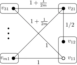
Figure 2: Hard instanceGGforGlobal Structure Representation. Edges not shown have weight∞.
optimal solution. For any non-optimal solutionT, definew((T)as the number of edges inT∗
which are missing inT.
The mutation operator can convert a non-optimal solutionT into the opti-mal solutionT∗with a sequence ofw((T)
≤m−1edge exchange operations. The probability that the mutation operator exchangesw((t)≤m−1edges in one mutation step is at least
Pr (Pois(1) =m−1) = 1/e(m−1)!.
In each exchange operation, if there areioptimal edges missing, then the probability that one of the missing optimal edges is inserted is at leasti/m2.
Af-ter the addition of an optimal edge, the probability of excluding a non-optimal edge is at least1/msince the largest cycle cannot be longer thanm. At most
m−1non-optimal edges must be exchanged in this manner. So the probability that the non-optimal solutionTwill be converted to the optimal solutionT∗
in one mutation step is at least
1
e(m−1)!· m−1
Y
i=1
i m2 ·
1
m ≥(1/e)m
−3(m−1).
So, the expected time to achieve an optimal solution is inO(m3(m−1)).
Fur-thermore, the probability that the optimal solution has not been created after
ekm3(m−1)iterations is
(1−(1/e)m−3(m−1))ekm3(m−1)
≤exp(−k).
We now present an instance which is hard to be solved by the tree based (1+1) EA. The instanceGG, illustrated in Figure 2, consists ofnnodes andm clusters. There are two central clusters denoted by V1 and V2. The cluster
m, contain a single nodevi1 each. The edges that connect the nodes v11 to
the peripheral cluster nodes have cost1. The edges that connectv21 to the
peripheral clusters have weight 1 + 1/2m. The edge that connects v12 and
v21 have weight1/2. All other edges have cost∞. Hence, if the tree based
(1+1) EA connects clusterV1andV2, then the dynamic programming algorithm
will choose nodev12.
In our analysis, we will use the following lemma on basic properties of the Poisson distribution with expectation1.
Lemma 4. IfK∼Pois(1), thenPr (K≥n)<2(e/n)n.
Proof. Using Stirling’s approximation of the factorial,
n!>√2πn(n/e)n>(n/e)n.
we obtain the simple bound
Pr (K≥n) =
∞ X
i=n 1
ei!
<
∞ X
i=n 1
i!
<
∞ X
i=n 1
n!
1
n+ 1
i−n
<(e/n)n
∞ X
i=0
1
n+ 1
i
= (e/n)n
1 + 1
n
.
Using the previous lemma, we are able to show that the tree based (1+1) EA finds it hard to optimizeGGwhen choosing spanning tree uniformly at random among all spanning trees having weight less then∞.
Theorem 5. Starting with a spanning tree chosen uniformly at random among all spanning trees that have cost less than∞, the expected optimization time of the tree based (1+1) EA onGGisΩ((m/e)m−1).
Proof. Consider the instance in Figure 2. In the following, edgee:={v12, v21}
is the edge which connects the two central clusters. The optimal solution cor-responds to the spanning tree which includes edgee, and where all all other clusters are connected to clusterV2. The solution where all peripheral clusters
are connected toV1, and where clusterV2is connected to one of the peripheral
clusters, is a local optimum.
1. The first type of failure occurs when the initial solution includes edgee.
2. The second type of failure occurs when less thanm/3of the peripheral clusters are connected to clusterV1in the initial solution.
3. The third type of failure occurs when the algorithm jumps directly to the optimal solution during the first((m−2)/3e)(m−2)/6iterations.
4. Finally, the fourth type of failure occurs if after iteration((m−2)/3e)(m−2)/6,
there exists a peripheral cluster which is not connected to clusterV1.
There arem−2peripheral clusters which must be connected to eitherV1or
V2. Additionally, clusterV1andV2must be connected. This connection can be
established either by adding edgee= (v12, v21), or by connecting a peripheral
cluster to bothV1 andV2. There are2m−2 spanning trees which contain edge
e, and(m−2)·2m−3 spanning trees which do not contain edge esince one
of them−2peripheral clusters will be connected to both central clusters and the others will be connected to only one. So, the probability that a uniformly chosen spanning tree includes edgeeisO(1/m), which is the probability of the first type of failure.
Now, we show that the probability of the second type of failure is at most
exp(−Ω(m)). Considering that the probability of a specific cluster is adjacent to V1 in the initial solution is larger than 1/2, the probability that less than
(m−2)/3clusters are connected to clusterV1in the initial solution is bounded
byexp(−Ω(m))using a Chernoff bound.
Assuming that type one and type two failures did not occur, the algorithm cannot accept new search points where a cluster which is originally connected toV1is instead connected toV2since it will create an extra cost of1/2m. The
only exception is if a type three failure occurs, i. e. the algorithm jumps directly to the optimal solution where all the peripheral clusters are connected toV2.
For a type three failure to occur, at least(m−2)/3clusters have to be modified simultaneously. Therefore, using Lemma 4, the probability of jumping directly to the optimal solution in a single step is bounded from above by
2(3e/(m−2))(m−2)/3.
Taking a phase length of((m−2)/3e)(m−2)/6into account, the probability
of a type three failure can be bounded from above using the union bound, as
((m−2)/3e)(m−2)/62(3e/(m
−2))(m−2)/3= (m/e)−Ω(m).
Now, it will be shown that the probability of a type four failure ise−Ω(m).
The probability that a single peripheral cluster which is connected to V2 is
switched toV1is bounded from below by
1 3·
1
e·
1
(m2−(m−1)) = Ω(1/m
Thus, the expected time between any such event isO(m2), and the expected
time until all of the at mostm−2 peripheral clusters are connected toV1 is
E[T′] =O(m3). By Markov’s inequality, it holds for any nonnegative random
variableXthat
Pr (X ≥k)≤E[kX].
The probability that it takes longer than
k= ((m−2)/3e)(m−2)/6
iterations is therefore no more than
E[T′]
k =O(m
3)
·((m−2)/3e)−(m−2)/6= (m/e)−Ω(m).
This proves our claim about the probability of failure event four.
If none of the above mentioned failures occur, we reach the local optimum where all the peripheral clusters are connected to clusterV1. From this point
on, the probability to jump to the optimal solution is by Lemma 4 no more than
2(e/(m−1))m−1
because it is necessary to make at leastm−1 edge exchanges to reach the optimum. The expected time to reach the optimal solution conditional on no failure is therefore more than(1/2)(m/e)m−1.
LetRbe the event that no failure occurs. By the law of total probability, it follows that the expected timeE[T]to reach the global optimum is
E[T]≥E[T|R] Pr (R) = Ω((m/e)m−1)(1
−O(1/m)) = Ω((m/e)m−1).
The previous theorem shows that there are instances for the cluster based (1+1) EA where the optimization time grows exponentially with the number of clusters. In the next section, we will compare the two different representations for GMSTP and show that they have complementary capabilities.
2.4
Complementary Abilities
the hard instance for one algorithm becomes easy to solve when giving it as an input to the other algorithm.
In Section 2.2, we have shown a lower bound ofΩ(nm)for the cluster based (1+1) EA using theSpanning Node Representation. The hard instanceGS for the cluster based (1+1) EA given in Figure 1 consists of a central cluster to which all the other clusters are connected. There are no other connections between the clusters. Hence, there is only one spanning tree when working with the
Global Structure Representation. The dynamic programming algorithm that runs on the lower layer of the tree based (1+1) EA therefore solves the problem in its first iteration.
The following theorem shows that these instances are easy to be optimised by the tree based (1+1) EA.
Theorem 6. The tree based (1+1) EA solves the instance GS in expected constant
time.
Proof. There is only a single tree over the cluster graph. Hence, the algorithm selects the optimal tree in the initial iteration.
For the tree based (1+1) EA, working with theGlobal Structure Representa-tion, we showed that it finds the instanceGGgiven in Figure 2 hard to solve. Working with theSpanning Nodes Representation, there is only one cluster that consists of two nodes where all the other clusters contain exactly one node. Hence, an optimal solution is obtained by computing a minimum spanning tree on the lower level if the right node in the cluster of two nodes is chosen. The following theorem summarises this and shows that this instance become easy when working with the cluster based (1+1) EA.
Theorem 7. The cluster based (1+1) EA solves the instanceGG in expected time
O(m).
Proof. Cluster V1 contains two nodes, and all other clusters contain a single
node. If the initial solution is not already the optimal solution, the correct node ofV1has to be selected using mutation. The node for the clusterV1is changed
with probability1/mand in such a step the correct node is selected with prob-ability1/2. Hence, the probability of a mutation leading to an optimal solution is at least21mand the expected waiting time for this event isO(m).
The investigations in this section show that the two examined representa-tions have complementary abilities. Switching from one representation to the other one can significantly reduce the runtime.
3
Generalised Travelling Salesman Problem
We now turn our attention to the NP-hard generalized traveling salesperson problem (GTSP). Given a complete graphG = (V, E, c)with a cost function
Algorithm 2Tour-based (1+1) EA
1: Choose a random permutationπ(which is also a Hamiltonian tour) of the
mgiven clusters.
2: Find the set of nodes P (one node in each cluster) to build the shortest path possible among those clusters with the given order, by means of any shortest path algorithm in timeO(n3).
3: whiletermination condition not satisfieddo 4: π′←π
5: fori∈[K]whereK∼1 +P ois(1)do
6: Choose two nodes fromπ′uniformly at random.
7: π′
←Perform theJumpwith the chosen nodes onπ′
8: end for
9: Find the set of nodesP′ = (p′
1, . . . , p′m)which minimizes the cost with respect toπ′
in the lower level 10: ifc(π′
)≤c(π)then 11: P ←P′
12: π←π′ 13: end if 14: end while
the goal is to find a cycle of minimal cost that contains exactly one node from each cluster.
The bi-level approach that we are studying is similar to the one discussed in the previous section. We investigate theGlobal Structure Representationwhich works on the complete graph H = (V′, E′) obtained from the input graph
G= (V, E, c). The nodevi ∈V′,1≤i≤m, represents the clusterViofG. The upper level solution in theGlobal Structure Representationis a Hamilto-nian tourπonHand the lower level solution is a set of nodesP = (p1, . . . , pm) withpi∈Vithat minimises the cost of a Hamiltonian tour which connects the clusters in the same way asπ. Given the restriction imposed by the Hamilto-nian tourπofH, finding the optimal set of nodesP can be done in timeO(n3)
by using any shortest path algorithm. One such algorithm isCluster Optimi-sationproposed initially by Fischetti et al (Fischetti et al., 1997) and is widely used in the literature. Letπ= (π1, . . . , πm)be a permutation on themclusters andpibe the chosen node for clusterVπi,1≤i≤m. Then the cost of the tour
πis given by
c(π) =c(pm, p1) +
m−1
X
i=1
c(pi, pi+1).
Our proposed algorithm starts with a random permutation of clusters which is always a Hamiltonian tourπ, in a complete graphH. In each iteration, a new solutionπ′
to1+P ois(1), whereP ois(1)denotes the Poisson distribution with expectation
1. Although we are using the jump operator in these investigations, we would like to mention that similar results can be obtained for other popular mutation operators such asexchangeandinversion.
Theorem 8.The expected optimization time of the tour based (1+1) EA isO(m!m2m).
Proof. We consider the probability of obtaining the optimal tour π∗
on the global graphH from an arbitrary tourπ. The number ofJumpoperations re-quired is at mostm(the number of clusters). The probability of picking the right node and moving it to the right position in each of thosemoperations is at least1/m2. We can obtain an optimal solution by carrying out a sequence of
mjump operations where theith operation jumps elementπ∗
i inπto position
i. Since the probability ofP ois(1) + 1 =mis1/(e(m−1)!), the probability of a specific sequence ofmJumpoperations to occur is bounded below by
1
e(m−1)! · 1
m2m.
Therefore, the expected waiting time for such a mutation is
1
e(m−1)!· 1
m2m
−1
=O(m!m2m)
which proves the upper bound on the expected optimization time.
Note that this upper bound depends on the number of clusters. Since the computational effort required to assess the lower level problem is poly-nomial in input size,O(n3), this implies that the proposed algorithm is a
fixed-parameter evolutionary algorithm for the GTSP problem and the fixed-parameterm, the number of clusters.
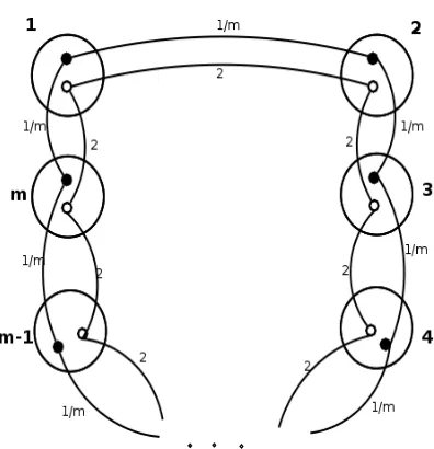
So far we have found an upper bound for the expected time of finding an optimal solution using the presented algorithm. In this section we will find a lower bound for the optimization time. Figure 3 illustrates an instance of GTSP,
GG, for which finding the optimal solution is difficult by means of the pre-sented bi-level evolutionary algorithm with Global Structure Representation. In this graph, each cluster has two nodes. On the upper layer a tour for clusters is found by the EA and on the lower layer the best node for that tour is found within each cluster. All white nodes (which represent sub-optimal nodes) are connected to each other, making any permutation of clusters a Hamiltonian tour even if the black nodes are not used. All such connections have a weight of1, except for those which are shown in the figure which have a weight of2. All edges between a black node and a white node and also all edges between black nodes have weightm2, except the ones presented in the figure which
have weight1/m. An optimal solution of cost1 uses only edges of cost1/m
Figure 3: Hard instanceGGfor GTSP withglobal structure representation
analysis it is just important that they do not share any edge with an optimal solution.
The clusters are numbered in the figure, and a measureS for evaluating cluster orders is based on this numbering: Letπ = (π1, . . . , πm)represent the permutation of clusters in the upper layer, thenS(π) = |{i | π(i+1 mod m) =
(πi+ 1) mod m}|indicates the similarity of the permutation with the optimal permutation. A large value ofS(π)means that many clusters inπare in the same order as in the optimal solution. Note thatS(π∗) = m
for an optimal solutionπ∗
. A solutionπwith S(π) = 0is locally optimal in the sense that there is no strictly better solution in the neighbourhood induced by the jump operator. The solutions withS(π) = 0form a plateau where all solutions differ from the optimal solution bymedges.
We first introduce a lemma that will later help us with the proof of the lower bound on the optimization time.
Lemma 9. Letπandπ′be two non-optimal cluster permutations for the instanceG
G.
IfS(π′
)> S(π)thenc(π′
)> c(π).
Proof. In the given instance, all white nodes are connected to each other with a maximum weight of 2. These connections ensure that any permutation of the clusters, can result in a Hamiltonian tour with a cost of at most2m. More-over, all connections between white nodes and black nodes have a weight of
m2. So the lower level will never choose a combination of white and black
nodes because the cost will be more thanm2while there is an option of
not choose any black nodes, because it will not be possible to use all the1/m
edges and somem2-weighted edges will be used again. Leta = S(π)be the
number of clusters adjacent to each other correctly from the right side (hav-ing the same right-side neighbour as in the Global Optimum) in a solutionπ. Thenb = m−ais the number of clusters which have a different neighbour on their right. Ifπis not the optimal solution, then the lower level will choose all white nodes. As a result,aedges with weight 2 andbedges with weight 1 will be used in that solution; therefore, the total cost of solutionπ will be
c(π) = 2a+b = 2a+m−a=m+a. Consider a solutionπ′
witha′ =S(π′)
andS(π′) > S(π)
. We havec(π′) =m+a′ > m+a =c(π)
which completes the proof.
Lemma 9 shows that any non-optimal offspring π′ of a solutionπis not
accepted if it is closer to an optimal solutionπ∗. This means that the algorithm
finds it hard to obtain an optimal solution forGGand leads to an exponential lower bound on the optimization time as shown in the following theorem.
Theorem 10. Starting with a permutation of clusters chosen uniformly at random, the optimisation time of the tour based (1+1) EA onGGisΩ((m2)
m
2)with probability
1−e−Ω(m).
Proof. ConsideringGGillustrated in Figure 3, the optimal solution is the tour comprising all edges with weightm1. We consider a typical run of the algorithm consisting of a phase ofT =Cm3steps whereCis an appropriate constant. For
the typical run we show the following:
1. A local optimumπwithS(π) = 0is reached with probability1−e−Ω(m)
2. The global optimal solution is not obtained with probability1−m−Ω(m)
Then we state that only a direct jump from the local optimum to the global optimum is possible, and the probability of this event isO(m−m/2).
First we show that with high probabilityS(πinit)≤εmholds for the initial solutionπinit, whereεis a small positive constant.
We count the number of permutations in which at leastεm,ε >0 a small constant, of cluster-neighbourhoods are correct.
We should selectεmof the clusters to be followed by their specific neigh-bour, and consider the number of different permutations ofm−εmclusters:
m εm
(m−εm)! (1)
Some solutions are double-counted in this expression, so the actual number of different solutions withS(π)≥εmis less than (1). Therefore, the probability of having more thanεmclusters followed by their specific cluster, is at most
m
εm
(m
−εm)!
m! = ((εm)!)
−1=O
εm
2
Hence, with probability1−O((εm2 )−εm2 ),S(π
init)≤εmholds and the initial solution has at at mostεmcorrectly ordered clusters.
Now we analyze the expected time to reach a solutionπwithS(π) = 0. The probability of a good ordering to change to a bad one is at least
1 e · k m ·
m2−m
m2
k
wherekis the number of edges which can be changed in each operation. For
jumpoperationkequals3. For allm >2, it holds thatm < m2
2 , so the
probabil-ity above is at least
1 e · 3 m · 1 2 3
= Ω(m−1)
Therefore, the expected time for each edge to be replaced with a bad edge is inO(m)and formedges it is inO(m2).
Now we consider a phase ofT = Cm3iterations and show that the local
optimum is reached with high probability.
LetC= 2C′and consider a phase of2C′m2iterations while assuming that
the local optimum is expected to be reached in timeC′m2. Then by means of
Markov’s Inequality we have
Pr(T′
>2C′
m2)≤12.
Repeating thismtimes, the probability of not reaching the local optimum is2−m. Therefore, the algorithm reaches the local optimum with probability 1−2−m= 1
−e−Ω(m)during the phase ofT =Cm3steps.
To prove that with high probability, the global optimum is not reached dur-ing the considered phase, note first that by Lemma 9, any jump to a solution closer to the optimum other than directly to the Global Optimum will be re-jected.
Furthermore, for the initial solutionS(πinit) ≤ εm. Therefore, only non-optimal solutionsπwithS(π)≤εmare accepted by the algorithm. In order to obtain an optimal solution the algorithm has to produce the optimal solution from a solutionπwithS(π) ≤ εmin a single mutation step. We now upper bound the probability of such a direct jump which changes at least(1−ε)m
clusters to their correct order. Such a move needs at least (1−ε)m
3 operations
in the same iteration. Taking into account that theseJumpoperations may be acceptable in any order, the probability of a direct jump is at most
1
e(1−ε)m
3
!. 1
m(1−2ε)m
·
(1−ε)m
3
! =m−Ω(m). (2)
So in a phase of O(m3)iterations the probability of having such a direct
So far we have shown that a local optimumπwithS(π) = 0is reached with probability1−e−Ω(m)within the firstT =Cm3iterations.
The probability of obtaining an optimal solution from a solution π with
S(π) = 0is at most
1
e m3
!· 1
mm2 ·
m
3
! =e−1
·m−m2
We now consider an additional phase of(m2)m2 steps after having obtained a local optimum. Using the union bound, the probability of reaching the global optimum in this phase is at most
m
2
m2
·e−1·m−m2
≤
1
2
m2
.
As a result, the probability of not reaching the optimal solution in these
(m2)m2 iterations is1−2−
m
2 = 1−e−Ω(m). Altogether, the optimization time is at least(m
2)
m
2 with probability1−e−Ω(m).
4
Discussion of Generalisations
The problems we have examined in this work are bilevel optimisation prob-lems where the upper level problem, namely theleader, and the lower level problem, thefollower, shares an objective function. The general bilevel opti-misation problem also includes the setting where the leader and the follower have different objectives. Given the decision of the leader, the follower makes a decision according to his objective function which might be conflicting with the objective function of the leader. An example of such a problem is where the leader places toll booths across a road network and the followers try to find the cheapest way from a pointAto a pointBby finding a path that avoids as many toll booths as possible. Here, the leader can only learn the objective func-tion value of its decision after the follower picks the optimum path. Unlike the GMSTP and GTSP, the objective functions of upper and lower level problems are conflicting in this toll booth problem.
For a given solution visited in the upper level problem, the evaluation cost is, in the worst case, the computational complexity of the lower level prob-lem. If the lower level problem can be solved in polynomial time, then a fixed-parameter bound on the the size of the upper level solution is sufficient for a fixed-parameter tractable problem. For when the upper level solution is bounded by a parameterkof the original problem, any global random search heuristic on the upper level problem will be able to find the optimal upper level solution in no more thanf(k)iterations for some functionf(k)and will make
f(k)·poly(n)basic operations in total.
In our case, theGlobal structure representationof GMSTP and GTSP, the size of an upper level solution is bounded above bym2since it is enough to
size ofmlog(n)to representwhich nodeis selected ineach cluster. If the solution size is restricted by a parameterm, uniform random search on the bitstring of lengthO(f(m))will find the optimal solution in2O(f(m))iterations in
expecta-tion. WithGlobal structure representation, if we pick our solutions uniformly at random the probability of picking a unique optimal solution is(1/2)m2
which will occur inO(m2m)time in expectation while uniform random search with the spanned node representation takesΩ(nm)trials in expectation.
Conclusions
Evolutionary bilevel optimization has gained an increasing interest in recent years. With this article we have contributed to the theoretical understanding by considering two classical NP-hard combinatorial optimization problems, namely the generalized minimum spanning tree problem and the generalized traveling salesperson problem. We studied evolutionary algorithms for the mentioned problems in the parameterized setting. Using parameterised com-putational complexity analysis of evolutionary algorithms for the generalized minimum spanning tree problem, we have examined two representations for the upper layer solutions and their corresponding deterministic algorithms for the lower layer. Our results show that theGlobal Structure Representationleads to fixed parameter evolutionary algorithms. By presenting hard instances for each of the two approaches, we have pointed out where they run into difficul-ties. Furthermore, we have shown that the two representations for the gener-alized minimum spanning tree problem are highly complementary by prov-ing that they are highly efficient on the hard instance of the other algorithm. After having achieved these results for the generalized minimum spanning tree problem, we turned our attending to the generalized traveling salesper-son problem. We showed that using the global structure representation leads to fixed parameter evolutionary algorithms with respect to the number of clus-ters. Furthermore, we pointed out a worst case instance where the optimization time grows exponential with respect to the number of clusters and discussed generalizations of the results.
References
Auger, A. and Doerr, B., editors (2011). Theory of Randomized Search Heuristics: Foundations and Recent Developments. World Scientific.
Corus, D., Lehre, P. K., and Neumann, F. (2013). The generalized minimum spanning tree problem: a parameterized complexity analysis of bi-level op-timisation. In Blum, C. and Alba, E., editors,GECCO, pages 519–526. ACM. Deb, K. and Sinha, A. (2009). Solving bilevel multi-objective optimization
Gandibleux, X., Hao, J.-K., and Sevaux, M., editors,EMO, volume 5467 of
Lecture Notes in Computer Science, pages 110–124. Springer.
Deb, K. and Sinha, A. (2010). An efficient and accurate solution method-ology for bilevel multi-objective programming problems using a hybrid evolutionary-local-search algorithm. Evolutionary Computation, 18(3):403– 449.
Downey, R. G. and Fellows, M. R. (1999). Parameterized Complexity. Springer-Verlag. 530 pp.
Fischetti, M., Salazar Gonz´alez, J. J., and Toth, P. (1997). A branch-and-cut algo-rithm for the symmetric generalized traveling salesman problem.Operations Research, 45(3):378–394.
Hu, B. and Raidl, G. R. (2011). An evolutionary algorithm with solution archive for the generalized minimum spanning tree problem. In Moreno-D´ıaz, R., Pichler, F., and Quesada-Arencibia, A., editors,EUROCAST (1), volume 6927 ofLecture Notes in Computer Science, pages 287–294. Springer.
Hu, B. and Raidl, G. R. (2012). An evolutionary algorithm with solution archives and bounding extension for the generalized minimum spanning tree problem. In Soule, T. and Moore, J. H., editors,GECCO, pages 393–400. ACM.
Koh, A. (2007). Solving transportation bi-level programs with differential evo-lution. InIEEE Congress on Evolutionary Computation, pages 2243–2250. IEEE. Kratsch, S., Lehre, P. K., Neumann, F., and Oliveto, P. S. (2010). Fixed parame-ter evolutionary algorithms and maximum leaf spanning trees: A matparame-ter of mutation. InProceedings of the Eleventh Conference on Parallel Problem Solving from Nature, pages 204–213.
Kratsch, S. and Neumann, F. (2013). Fixed-parameter evolutionary algorithms and the vertex cover problem.Algorithmica, 65(4):754–771.
Legillon, F., Liefooghe, A., and Talbi, E.-G. (2012). Cobra: A cooperative coevo-lutionary algorithm for bi-level optimization. InIEEE Congress on Evolution-ary Computation, pages 1–8. IEEE.
Motwani, R. and Raghavan, P. (1995).Randomized Algorithms. Cambridge Uni-versity Press.
Myung, Y.-S., ho Lee, C., and wan Tcha, D. (1995). On the generalized mini-mum spanning tree problem.Networks, 26(4):231–241.
Pop, P. C. (2004). New models of the generalized minimum spanning tree prob-lem.J. Math. Model. Algorithms, 3(2):153–166.
Sutton, A. M. and Neumann, F. (2012a). A parameterized runtime analysis of evolutionary algorithms for the euclidean traveling salesperson problem. In Hoffmann, J. and Selman, B., editors,AAAI. AAAI Press. Extended technical report available at http://arxiv.org/abs/1207.0578.