Predicting Hydration Gibbs Energies of Alkyl-aromatics Using
Molecular Simulation: A Comparison of Current Force Fields and the
Development of a New Parameter Set for Accurate Solvation Data
Nuno M. Garrido1, Miguel Jorge1, António J. Queimada1, José R. B. Gomes2,
Ioannis G. Economou3 and Eugénia A. Macedo1,*
1. LSRE Laboratory of Separation and Reaction Engineering, Departamento de
Engenharia Química, Faculdade de Engenharia, Universidade do Porto, Rua do Dr.
Roberto Frias, 4200 - 465 Porto, Portugal
2. CICECO, Department of Chemistry, University of Aveiro, Campus Universitário de
Santiago, Aveiro 3810-193, Portugal
3. The Petroleum Institute, Department of Chemical Engineering, PO Box 2533, Abu
Dhabi, United Arab Emirates
*
Author to whom all correspondence should be addressed at: [email protected]
Manuscript submitted for publication in Physical Chemistry Chemical Physics
ABSTRACT
1. Introduction
Over the last decades, free energy calculations have continuously become more important in the chemical and biochemical fields, as noted in several literature reviews1-4. Free energy studies allow scientists and engineers to achieve microscopic-level insights into the behavior of complex systems that may be helpful in chemical process design, e.g. to estimate important properties such as solubility5,6 or partition coefficients7,8. Accurate predictions of the Gibbs energy of solvation, also called solvation free energy, have the capacity to revolutionize several fields, predominantly in the pharmaceutical industry and/or in biological chemistry9,10. In this context, molecular simulation has emerged as a highly promising method to estimate free energies of drug-like molecules10,11. The importance and at the same time the difficulty of connecting classical atomistic models to experimental results in order to predict the Gibbs energy of solvation is also illustrated in a recent blind challenge12.
One of the major drawbacks of free energy predictions from molecular simulations is that they tend to be quite sensitive to the force field and in some cases to the simulation parameters (cutoff radii, treatment of long-range electrostatics, etc.).13 For this reason, several studies have focused on comparing existing force fields14-17 or on fine-tuning existing ones18-20 for solvation Gibbs energy predictions. Some of those studies have shown that the electrostatic contribution to the calculated Gibbs energy, commonly dependent on an adequate assignment of partial charges to each atom or group of atoms, is particularly prone to uncertainties, and sometimes hinders the transferability of the force field parameters21,22. In fact, an important shortcoming of fixed-charge force fields is that they do not normally take into account the different polarization environment when a molecule is transferred from the liquid phase to the gas phase (or vice-versa)23,24.
the total hydration energy for polar solutes21,22. Our strategy is to systematically study a homologous series of compounds, rather than to apply the usual approach of testing the force fields against a large database of solutes with many different functional moieties. In this way, we hope to identify more easily the reasons for the success or failure of certain parameter sets, and to establish a well-defined set of rules for force field development.
In the present work, we focus on the aqueous behavior of benzene and several alkyl-substituted aromatics: mono-, di- and tri-substituted alkylbenzenes. Such aromatic fragments are widely present in chemical and pharmaceutical compounds, biological assemblies and petrochemical systems. Xylenes are a particular family of di-substituted alkylbenzene isomers that are used as large scale industrial solvents and intermediates for many derivatives, e.g, p-xylene is used in the polyester industry. Besides their importance as industrial chemicals, aromatic compounds were also found to play a key role in biochemistry26-28. This class of compounds is also particularly interesting from a theoretical point of view, as aromatic interactions are usually difficult to quantify experimentally29.To the best of our knowledge there is no published systematic study about the prediction of the Gibbs energy of hydration of alkyl-aromatic compounds from molecular simulation. Thus, in the first part of this work we predict the Gibbs energies of hydration of benzene and five mono-substituted alkyl-benzenes using five current force field parameter sets from the TraPPE, Gromos and OPLS families.
The TraPPE force field was originally developed under a UA philosophy, where both aromatic CH and aliphatic CHx groups were treated as pseudo-atoms whose
molecular weights are equivalent to those of the whole fragment (henceforth denoted by TraPPE-UA31-34). More recently, an EH version of the TraPPE force-field was proposed for benzene35 and we have also decided to test this version of TraPPE (henceforth denoted by TraPPE-EH). However, this force field has not yet been extended to alkyl-aromatic compounds. Likewise, the Gromos biomolecular force field was originally developed as a united atom force field36 (Gromos-UA). However, recent developments have provided parameters for an EH description of the aromatic CH groups (Gromos-EH, version 53A537), which were parameterized to reproduce, among other properties, the Gibbs energy of hydration of amino acids containing aromatic groups37. Finally, although starting with a UA description, the Optimized Potential for Liquid Simulations (OPLS)30 force field quickly became popular with its AA description of the solute molecules. Moreover, for aromatic molecules the OPLS-UA model was not parameterized. One of the purposes of this paper is to understand how accurate the current parameter sets are in reproducing experimental hydration energies, and to evaluate the need for using optimized parameters to correctly achieve hydration data predictions.
In the second part of this paper, we attempt to improve the prediction of hydration energies, by generating a new charge set for an EH model for alkylbenzenes, based on the recent TraPPE-EH force field35, using information from natural population analysis (NPA) of density functional theory (DFT) calculations. NPA is a method for deriving charges and orbital populations of atoms in a molecular system, based on a natural bond orbital analysis38.The new charge set is obtained by scaling the calculated gas-phase charges to fit the experimental Gibbs energy of solvation of benzene and of 1,3,5-trimethylbenzene. A new rule for assigning partial atomic charges for multisubstituted alkyl-aromatic compounds is also presented. The ability of this new charge set to predict solvation energies of several other alkyl-aromatic compounds is examined.
3.2 is dedicated to improving force field parameters for better reproducing experimental hydration energies. Finally, our main conclusions are summarized in Section 4.
2. Theoretical and Computational Details
2.1. Calculation of the Gibbs energy of hydration
The Gibbs energy of hydration can be seen as the total reversible work required to transfer a solute molecule from the ideal gas phase to water, at constant pressure and temperature, representing the infinite dilution chemical potential. Free energies can be calculated for an appropriate molecular model by carrying out molecular dynamics (MD) simulations and a thermodynamic integration (TI) procedure. Based on a thermodynamic cycle, the Gibbs energy of hydration, ∆hydG, is estimated from
simulations in which solute-solvent interactions are progressively turned off. This has normally been accomplished by carrying out two separate simulations, one in solution (where both intra- and inter-molecular contributions are turned-off) and another one in vacuum (to subtract the intra-molecular contribution)39. Details of this methodology can be found in a previous publication13. However, a new feature in the MD GROMACS 4.0 suite40 allows for these intermolecular solute-solvent interactions to be quantified by solely running a liquid phase simulation, thus avoiding the need for a vacuum step. The latter approach was adopted here.
The TI algorithm, free of hysteresis, has been described in detail in previous publications41-43. Briefly, if we consider any two generic well-defined states, the total Hamiltonian of the system can be made a function of a coupling parameter, λ, and used
to describe the transition between those two states – in this case, an initial fully interacting system and a final “dummy” state where all solute-solvent interactions are turned off. Considering several discrete and independent λ values, equilibrium averages
can be used to evaluate derivatives of the Gibbs energy with respect to λ. One then
integrates these derivatives along a continuous path connecting the initial and final states to obtain the Gibbs energy between them.
to avoid charge-fusion effects14,44 we have first turned off the electrostatic interactions and then the LJ interactions. The total Gibbs energy of hydration can then be estimated from:
( )
( )
( )
1 1 1
0 0 0
Total Elec LJ
hydG d d d
λ λ λ
λ λ λ
λ λ λ
λ λ λ
∂ ∂ ∂
∆ = − = − +
∂ ∂ ∂
∫
H∫
H∫
H (1)A MD simulation was performed for each discrete λ value, ranging from λ = 0
(fully interacting solute) to λ = 1 (non-interacting solute). We have used 5 λ values for
the electrostatic decoupling and 15 λ points to evaluate the LJ contribution. As
demonstrated in a previous work, this choice of intermediate states ensures sufficient accuracy in the free energy calculations45. The integration of the LJ Hamiltonian derivatives was carried out by fitting the data to a physically-based approximation to the cavity formation and dispersion interaction terms and then integrating the curve analytically45. The fitting function is:
( )
2 2 20 1 2
3 4 4
LJ
A A
A A
A A A
λ
λ λ
λ λ λ
∂ = + − + ∂ − + H (2)
where Ai are fitting parameters45. In all cases we have employed non-linear weighted least squares fittings of the simulation data. Correlation coefficients above 0.99 and a global RMS error of 0.3 kJ/mol were obtained. This integration procedure was shown to increase the precision of the calculated hydration energies while decreasing the number of necessary intermediate points45. Simpson’s rule was used for the integration of the electrostatic component. During the decoupling process, the electrostatic interactions were linearly interpolated between neighboring states while the LJ interactions were interpolated via soft-core interactions46, with parameters given in our previous publications13. This soft-core dependence eliminates singularities in the calculation as the LJ interactions are turned off 47.
2.2.Molecular Dynamics Simulations
GROMACS software40 using the leap-frog Verlet integration algorithm48 with a time step of 2 fs to integrate Newton’s equations of motion. Simulations were performed using periodic boundary conditions in all directions. Covalent bonds involving hydrogen atoms were constrained using the LINCS algorithm49 while the water geometry was fixed with the SETTLE algorithm50. For efficiency reasons (see reference51 for details), the reaction-field method52, which approximates the medium beyond a cut-off distance of 1 nm by a dielectric continuum of uniform permittivity, was used to handle long-range electrostatics. The dielectric constant was adjusted to be the permittivity of each solvent or pure component. The Ewald summation method was applied in a few test cases and the resulting hydration energies were practically the same as with the reaction field method (difference of at most 0.2 kJ/mol). The remaining cut-off radii were 1 nm for the short-range neighbor list and a 0.8-0.9 nm switched cut-cut-off for the LJ interactions. We have also applied long range dispersion corrections for energy and pressure14.
In the case of free energy calculations, solvated systems consisted of one solute molecule and 500 water molecules at 298 K and 1 bar. As discussed in several previous studies, the choice of the water model may have implications in the final predicted Gibbs energy15,17,21,53. In the present work we have decided to use the Modified Extended Simple Point Charge (MSPC/E)54 model for the simulation of water. MSPC/E is an accurate force field for pure water and aqueous phase equilibria thermodynamic properties, and includes a polarization correction expected to improve hydration energy predictions. A comparison of the free energy results predicted with the MSPC/E and SPC/E55 water models was reported previously51. Nevertheless, we have also performed some tests with the TIP4P56 water model in this paper, as discussed in Section 3.2.
finally a 5 ns NpT production stage. It is worth noticing that 5 ns is considered to be enough to observe several transitions between stable configurations, indicating sufficient sampling of torsional degrees of freedom, even for complex solutes.13 Nevertheless, this point was carefully confirmed in this work for the longer n -alkylbenzenes, where several transitions between different torsional configurations were verified. All simulations were performed in triplicate, or in the case of the larger molecules in quintuplicate, in order to obtain statistically meaningful results.
For the estimation of the pure component properties we have employed the Nosé-Hoover thermostat60,61 for temperature coupling using a time constant of 1 ps, and the Parrinello-Rahman approach62 with a time constant of 2 ps to enforce pressure coupling. The reference pressure was set to 1 bar and the compressibility was set according to the fluid under evaluation (data from Cibulka and Takagi63). Each simulation box contained 512 molecules and had equilibrated box dimensions ranging from 4.19 to 5.14 nm. Liquid densities were directly obtained from the GROMACS suite using the g_energy64
tool, while heats of vaporization were estimated by taking the difference of enthalpy in the vapor and liquid phases:
vapH Eg EL RT
∆ = − + (3)
where, Egis the total energy in the gas phase and ELis the total energy per mole in the
liquid phase. Although other approaches for computing the heat of vaporization exist65, equation (3) is sufficiently accurate for our purposes. Vacuum (gas phase) simulations were conducted without cutoffs or periodic boundary conditions for 50 ns.
2.3. Density Functional Theory Calculations
The gas-phase geometries of all benzene derivatives considered in this work were optimized, using very tight convergence criteria (opt=verytight and int=ultrafine
from benzene71,72. The atomic charges were calculated i) from a natural population analysis73 (NPA) of the natural atomic orbitals (NAO) obtained by using the atomic blocks of the density matrix averaged over the spatial directions, e.g. px, py, pz orbitals, and ii) from the application of the CHelpG scheme74, based on the fitting of charges to the electrostatic potential calculated in a regularly spaced grid of points around the molecule under the constraint that the dipole moment is preserved. All charges thus calculated are provided in the Supporting Information (Tables S5 to S12).
3. Results and Discussion
3.1. Prediction of ∆∆∆∆hydG using current force field parameter sets
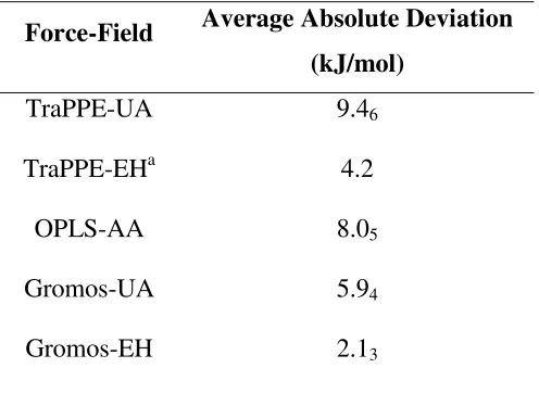
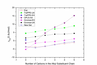
The Gibbs energy of hydration of benzene (BZ) and several mono-substituted alkylbenzenes, namely methylbenzene (MB), ethylbenzene (EB), propylbenzene (PB), butylbenzene (BB) and pentylbenzene (PeB), were initially estimated using the five parameter sets already mentioned: TraPPE-UA/EH, Gromos-UA/EH and OPLS-AA. Gibbs energy of hydration results using these force fields are presented in Tables S1-S4 of the Supporting Information and illustrated in Figure 1, while absolute average deviations (AAD) are summarized in Table 1. From these results one may generally conclude that with the exception of Gromos-EH version 53A6, which was specifically reparameterized to fit hydration energies, none of the current force field parameter sets are able to accurately predict the Gibbs energy of hydration of our molecular test set. Moreover, it is clear that OPLS-AA, in spite of its increased number of degrees of freedom arising from the all-atom description, is not able to accurately describe the Gibbs energy of hydration. Although it provides a reasonable prediction for BZ, it significantly overestimates the increase in free energy with the degree of substitution. Similar results were obtained for the hydration of alkanes7 suggesting that the shortcoming may arise from a deficiency in the parameterization of the LJ component in this force field.
shortcoming of the UA force fields is due to the fact that they neglect the electrostatic component of the interaction potential (all partial charges are set to zero), which is observed to be important in the solvation of aromatic solutes. Nevertheless, one may notice that the effect of increasing the alkyl chain length on going from toluene (methylbenzene) to pentylbenzene is correctly captured by both UA force fields, particularly in the case of TraPPE-UA. Because this series is generated by inserting neutral CHx groups into the substituent chain, it is expected that the electrostatic component will be approximately the same for all solutes, and thus the free energy differences between them should be dominated by changes in the LJ component. Since the relative Gibbs energy between subsequent members of the series is adequately captured, it can be concluded that the LJ component of the Gibbs energy is well described by the UA force fields. The current TraPPE LJ force field parameters are thus a good starting point for a further refinement in order to better reproduce hydration energies.
Dramatic quantitative improvements (by about 5 kJ/mol, see Table 1) in the Gibbs energy predictions can be obtained when an explicit hydrogen approach (which includes point charges, as in the case of TraPPE-EH and Gromos-EH) is used to describe the aromatic ring, maintaining the UA description of the alkyl substituents. Nevertheless, the TraPPE-EH prediction for BZ still falls short of the experimental hydration energy. In the case of the Gromos-EH force field, the predictions are quantitatively much better for the entire series (on average 3.8 kJ/mol closer to experiment when compared to the united-atom version – Table 1), but the experimental trend from benzene to toluene is not correctly described. Looking at the experimental data (∆hydGexp is more negative for
3.2. A new parameter set for accurate ∆∆∆∆hydG predictions
Our starting point is to describe the benzene ∆hydGexp by deriving new parameters
modifying TraPPE-EH to obtain a better match to the experimental Gibbs energy of hydration. We have seen that the electrostatic term, which usually plays a major role in bio-molecular systems22, seems to be incorrectly captured by the original charges in TraPPE-EH, as shown in Figure 1. This is not as unexpected as it may seem, if we consider that the experimental hydration energy includes additional contributions that arise from the change in polarization environment when moving from the gas phase to water, which are not captured by fixed-charge force fields. Indeed, the process described in section 2.1 computes the free energy to hydrate a molecular model of the solute in water, while holding its charge distribution fixed. However, in a real solvation process the electrostatic potential of the solute changes in response to the change in the polarization environment. Polarizable models can explicitly account for this change, but they are much more computationally demanding and are thus currently inappropriate for routine solvation free energy calculations. In the following, we will try to account for polarization effects in an approximate way using fixed-charge models. Swope et al.75,76 have recently presented a detailed analysis of this subject, and we will mostly follow their reasoning here.
polarization environment in the actual solvent of interest (in this case, water) can be significantly different. Thus, in principle one must also account for the free energy cost of changing this pure-component description into one that adequately represents the “experimental” solute in the solvent phase (the branch on the right-hand side of the cycle). Finally, it is worth mentioning that we follow Swope et al.75 in assuming that the model is able to sample the entire configuration space available to the “experimental” solute, so that all restructuring free energy contributions are zero.
Swope et al.75,76 went on to develop accurate expressions for estimating ∆GPolG for
fixed-charge models. A simplified form of those expressions, equation (4), has been used previously, for example in the development of the SPC/E water model55.
(
)
22
L G
G Pol
G µ µ
α −
∆ = (4)
In the above expression, µG is the dipole moment of the solute in the gas phase, µL is the
corresponding dipole moment in the liquid phase, and α is the isotropic polarizability. We have applied equation (4) to estimate this contribution for several alkyl-aromatic solutes, and found the energies to be lower than 0.1 kJ/mol, which is below the statistical error of the simulations (see below). This agrees with Swope et al.75, who found that the polarization contribution was practically negligible for toluene. Based on these results, the ∆GPolG contribution will be neglected in the remainder of this paper. It should be noted, however, that for more polar solutes the gas-phase polarization contribution is likely to be important and should be taken into account.
field, where different charges are fitted to reproduce Gibbs energy of solvation in solvents of different polarity37. This fact and the comparison we carried out in section 3.1 for standard “pure-component” force fields strongly suggest that ∆GPolL is non-negligible. Unfortunately, it is not straightforward to estimate this contribution in a similar way as for G
Pol G
∆ , since in the former case the change in polarization of the
solute will also change the solvent structure and the solute-solvent interaction energy in a non-trivial way75.
important to reiterate that the new charges derived here include the effect of a change in the polarization environment only implicitly.
• The Gibbs Energy of Hydration of Benzene
Due to the symmetry of the benzene ring, each CH aromatic group must be neutral, and so the charges assigned to the carbon and to the hydrogen atoms by the NPA method are symmetric (see Table S5). The scaling factor was estimated by fitting simulation results to the experimental Gibbs energy of hydration of benzene. We have analyzed the sensitivity of the electrostatic contribution to the hydration energy by testing 8 different values of the scaling factor, implying a range of charges from 0.055≤qH ≤0.155. From this analysis, we have verified that the system responds under a second order polynomial, going through the origin (see Figure S1 for details). Such a quadratic behavior of the electrostatic free energy is to be expected and has been reported before83, but it is nevertheless useful for charge-fitting purposes. In order to match the experimental Gibbs energy of hydration, we propose the following parameters for benzene: 0.1225
aro aro
C H
q = −q = − , which yield an electrostatic
contribution of ∆GbenzeneC = −9.13 kJ/mol and a ∆hydGbenzene = −3.6 kJ/mol. These charges were obtained by multiplying the NPA benzene partial charges by a scaling factor,
0.5
P
k = . As described above, this scaling factor accounts for limitations of the NPA method to accurately reproduce the electrostatic potential of the molecule, but also takes into account the change of environment from the gas phase to the aqueous phase, which may have a strong effect on the values of the effective point charges. Given the importance of these effects in a highly polar solvent such as water, it is not surprising to find a scaling factor of 0.5.
Previous work has shown that the choice of water model may have a significant effect on Gibbs energy of hydration predictions15. Even though it is beyond the scope of the present work to perform an exhaustive analysis of these effects, we have tested the current benzene parameters in a different water model. Thus, for the TIP4P water model we have obtained Calc4 LJ4 C 4 5.6 9.2 3.6
hydGTIP P GTIP P GTIP P
∆ = ∆ + ∆ = − = − kJ/mol, which is to
• The Gibbs Energy of Hydration of Substituted Aromatics
Having determined the optimal charges for BZ, in a second stage we addressed the Gibbs energy of hydration of toluene, longer mono-substituted alkylbenzenes and multi-substituted aromatics. As observed both in the trend from MB to PeB, shown in Figure 1, and in a previous study for alkanes7, the TraPPE-UA force field is able to correctly describe the non-polar component of the hydration energy for the series of alkanes or alkyl substituents, i.e., the TraPPE-UA force field reproduces the experimental trends in the relative Gibbs energy of solvation of the series MB to PeB. Thus, for all the alkyl substituents, we took the LJ parameters from this force field32,33 and kept them unchanged throughout our subsequent analysis. With these LJ parameters we then focused on the electrostatic component of the hydration energy.
Substituted aromatics can be “built” by replacing one (or more) aromatic hydrogens with a given alkyl group. Such a substitution obviously changes the electrostatic potential of the substituted aromatic carbon(s) and of the corresponding alkyl substituent(s), but may also induce changes in the charge distribution of the rest of the aromatic ring. When inserting a substituent in the aromatic ring, it is expected that the charge symmetry in the ring will suffer a disruption. The information extracted from DFT analysis shows that, for example, the inclusion of a CH3 group into the BZ ring to yield MB or the inclusion of a C2H5 into the BZ ring to yield EB, promotes a delocalization of the charges in the remaining aromatic sites. Concretely, in both cases the carbons located in ortho- and meta- positions relative to the substituted carbon become slightly more positive while the carbon in para- position becomes more negative (see Tables S6 and S7, respectively). As for hydrogens, those in meta- and
para- positions remain practically unchanged while the ortho-hydrogen becomes less polar.
Although the NPA analysis provides interesting insight regarding the effect of substituents on the charge distribution within the aromatic ring, it is difficult to directly apply NPA charges to the substituted carbon and alkyl substituents. This is because the NPA/DFT calculations naturally consider an all-atom description of the aliphatic groups, while our classical model adopts a united-atom approach. Simply adding up the NPA point charges of each CHx group present in the different substituent chains will
(see Tables S6-S8), which will strongly underestimate the electrostatic contribution to the hydration energy.
In order to determine the charge assigned to the substituted carbon atoms for the different multisubstituted alkylbenzenes we have determined the optimal value of this charge by fitting the hydration energy of 1,3,5-trimethylbenzene (TMB). For the non-substituted carbons and hydrogens we use the scaled NPA charges (kP = 0.5). We have thus gradually changed the charge of the (C)-CHx carbon (the charge of the CHx group
is also adjusted, to keep the whole molecule neutral) until the experimental TMB Gibbs energy of hydration was reproduced. Once more, we obtained a quadratic dependence of the TMB Gibbs energy of hydration with the carbon charge (see Figure S2). The optimal charge for the substituted aromatic carbon was found to be
( x)
C CH
q − = -0.107 (Table 2) and the corresponding TMB Gibbs energy of hydration was
-3.8 kJ/mol.
If we simply transfer this charge on the substituted carbon to several other mono-, di- and tri-substituted aromatics, we still assume that the effect of each substitution on that charge is independent of other substitutions elsewhere in the ring (i.e., the charge is directly transferred from TMB to the other solutes). Instead, we have attempted to devise a general rule for determining the contribution of each substitution to the charge on neighboring atoms, based on an analysis of the NPA charges.
3
0 BZ
i P i j j
j
q k q δ N
=
= × +
∑
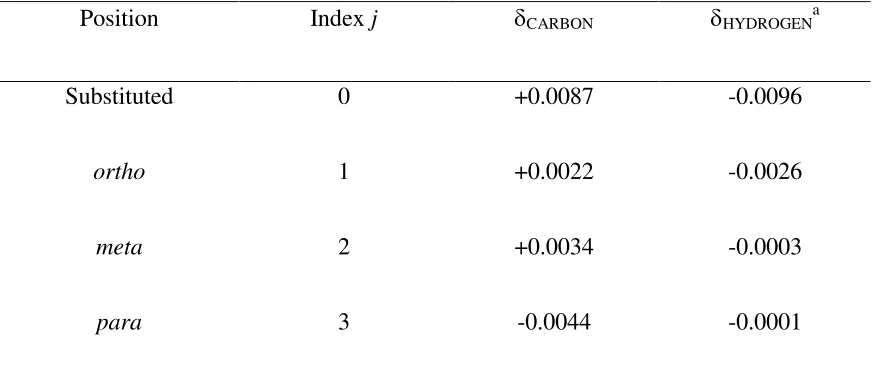
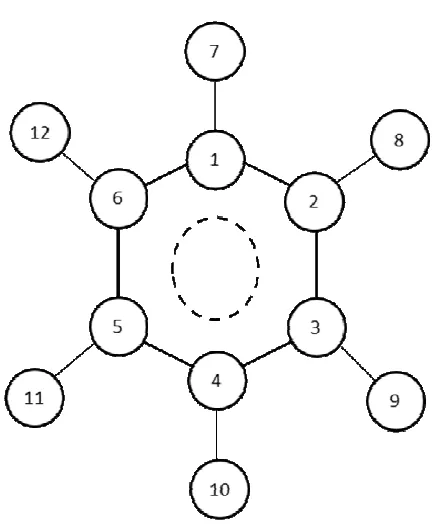
(5)where qi is the charge on site i (with numbers given in Figure 3), qiBZ is the
corresponding charge in the benzene molecule, δj is the charge increment caused by a
substituent at position j, and Nj is the total number of substituents at position j (j = 1,2,3
for ortho, meta and para substitution, respectively, and j = 0 for the substituted C-CHx group). The charge increments for each substituent position, shown in Table 3, were adjusted to provide the best possible match to the scaled NPA charges for the 3 compounds mentioned above. Point charges estimated using equation 4 were in excellent agreement with the scaled NPA charges for all compounds of the test set (RMS error lower than 0.0001 a.u.). Remaining CHx groups (e.g terminal CH3 groups in
EB, C2H5 in PB, etc.) were considered to be neutral, as one might expect.
The above procedure involves simply determining, for each atom of a given alkyl-aromatic molecule, the corresponding values of Nj. Equation (5) is then applied to
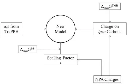
each atom, starting from the corresponding benzene charges and adding the contributions due to each substituent, to obtain the new charge set. For example, in TMB the charge on each non-substituted carbon atoms takes into account the contribution of one substituent in para position plus two substituents in ortho position. In the Supporting Information, we present an example (tutorial) of this calculation procedure for 1,2,4-trimethylbenzene. In Figure 4 we summarize the procedure followed to derive this new charge set and list the different quantities used as input data during its development. In Table 2 we give the detailed charge set of parameters proposed for the different compounds.
proposed here for parameterizing point charges has a significant potential to improve the capacity of current force fields to predict Gibbs energy of hydration. Moreover, the rule presented by equation (5) has the added advantages of eliminating the unnecessary assumption of fixed charge on every substituted carbon atom and providing a simple guideline for extrapolating the charge assignment to any multi-substituted alkyl-aromatic molecule.
Although the main aim of our parameterization of the point charges for alkyl-aromatic solutes is to predict Gibbs energies of hydration, we have also made a short test to evaluate how the new parameters perform for thermodynamic properties of pure liquids, namely their ability to predict i) liquid density in a wide temperature range and ii) enthalpy of vaporization. Additionally, we have tested the impact of force field changes on the structure of pure liquid benzene by computing radial distribution functions (RDFs). The calculated solvent densities from NpT MD and the heats of vaporization at various temperatures are shown in Supporting Information in Tables S13 and S14, respectively. Reported results enable to observe that the new charge set also allows estimating liquid densities and vaporization enthalpies for the test set in good agreement with the experimental data, i.e., a global deviation of 2% for liquid densities in the overall temperature range and a global AAD of 1.4 kJ/mol for the enthalpies. The structure of liquid benzene can be observed in several RDFs, which were calculated and are presented in Figure S3 of the Supporting Information. For the case of the computed aromatic Carbon – Carbon interactions (C-C curve), the agreement with experimental data available from X-ray diffraction84 is good. Moreover, both the experimental peaks in the 0.5-0.6 nm region and the shoulder around 0.7 nm are reproduced in the calculated data. The C-H and H-H functions are also similar to the ones obtained in previous calculations85,86. All three curves are practically indistinguishable from the corresponding RDFs obtained with the original TraPPE-EH model.
4. Conclusions
A better performance was obtained when information from normal population analysis of DFT calculations was used to describe charge delocalization within the aromatic ring induced by alkyl substitutions. Although it is premature to recommend NPA charges as the method of choice for force field parameterization, since our study focuses only on a single class of solutes, the good performance observed here is rather encouraging. Other methods for computing point charges should be tested in the near future and the range of solute types should be expanded to include more polar molecules.
NPA charges were multiplied by a constant scaling factor to account for the change of environment on moving from the gas phase to the aqueous phase, and this scaling factor was optimized by fitting the benzene hydration energy. An optimization of the charge on the substituted carbon atom was also found to improve performance. At this point, we cannot be sure if the same scaling factor applies for the Gibbs energy of hydration of more polar molecules. Regarding solvation in different solvents, it is likely that a different factor will need to be employed to account for a different solvation environment. Further studies are needed to clarify these issues.
As a result of our study, we have proposed a general rule for assigning point charges to any alkyl-aromatic solute, based on charge increments caused by each substitution. This new charge set was able to predict experimental hydration energies of several aromatic compounds with remarkable accuracy. In principle, this rule could be extended to other types of substituents (e.g., halogen atoms, hydroxyl groups, etc.), with appropriate changes in the increment parameters. The new framework presented here for the development of point charges enables accurate predictions of Gibbs energies of hydration using molecular simulation and thermodynamic integration. In future publications, we intend to extend this framework to molecules containing other functional groups and possibly to other solvents.
Supporting Information Available:
of vaporization using the new data set are also included. Finally, computed RDFs for liquid benzene are also shown.
Acknowledgments:
7. Cited References
(1) Kollman, P. A. Chem. Rev. 1993, 93, 2395.
(2) Jorgensen, W. L.; Thomas, L. L. J. Chem. Theory Comput. 2008, 4, 869.
(3) Beveridge, D. L.; Dicapua, F. M. Annu. Rev. Biophys. Biophys. Chem. 1989, 18, 431.
(4) Gilson, M.; Zhou, H. Ann. Rev. Biophys. Biomol. Struct. 2007, 36, 21.
(5) Westergren, J.; Lindfors, L.; Hoglund, T.; Luder, K.; Nordholm, S.; Kjellander, R. J. Phys. Chem. B 2007, 111, 1872.
(6) Palmer, D. S.; Llinas, A.; Morao, I.; Day, G. M.; Goodman, J. M.; Glen, R. C.; Mitchell, J. B. O. Molecular Pharmaceutics 2008, 5, 266.
(7) Garrido, N. M.; Queimada, A. J.; Jorge, M.; Macedo, E. A.; Economou, I. G. J. Chem. Theory Comput. 2009, 5, 2436.
(8) Garrido, N. M.; Jorge, M.; Queimada, A. J.; Macedo, E. A.; Economou, I. G.
Phys. Chem. Chem. Phys. 2011, DOI: 10.1039/c1cp20110g.
(9) Shirts, M. R.; Mobley, D. L.; Chodera, J. D. Ann Rep Comput Chem 2007, 3, 41. (10) Jorgensen, W. L. Science 2004, 303, 1813.
(11) Jorgensen, W. L.; Duffy, E. M. Bioorg. Med. Chem. Lett. 2000, 10, 1155. (12) Guthrie, J. P. J. Phys. Chem. B 2009, 113, 4501.
(13) Garrido, N. M.; Jorge, M.; Queimada, A. J.; Economou, I. G.; Macedo, E. A.
Fluid Phase Equilib 2010, 289, 148.
(14) Shirts, M. R.; Pitera, J. W.; Swope, W. C.; Pande, V. S. J. Chem. Phys. 2003,
119, 5740.
(15) Shirts, M. R.; Pande, V. S. J. Chem. Phys. 2005, 122, 134508.
(16) Mobley, D. L.; Bayly, C. I.; Cooper, M. D.; Shirts, M. R.; Dill, K. A. J. Chem. Theory Comput. 2009, 5, 350.
(17) Hess, B.; van der Vegt, N. F. A. J. Phys. Chem. B 2006, 110, 17616. (18) Davis, J. E.; Patel, S. Chem. Phys. Lett. 2010, 484, 173.
(19) Udier-Blagovic, M.; De Tirado, P. M.; Pearlman, S. A.; Jorgensen, W. L. J. Comp. Chem. 2004, 25, 1322.
(20) Rizzo, R. C.; Jorgensen, W. L. J. Am. Chem. Soc. 1999, 121, 4827.
(21) Mobley, D. L.; Dumont, E.; Chodera, J. D.; Dill, K. A. J. Phys. Chem. B 2007,
(22) van Gunsteren, W. F.; Bakowies, D.; Baron, R.; Chandrasekhar, I.; Christen, M.; Daura, X.; Gee, P.; Geerke, D. P.; Glättli, A.; Hünenberger, P. H.; Kastenholz, M. A.; Oostenbrink, C.; Schenk, M.; Trzesniak, D.; van der Vegt, N. F. A.; Yu, H. B. Angew. Chem. Int. Ed. 2006, 45, 4064.
(23) Swope, W. C.; Horn, H. W.; Rice, J. E. J. Phys. Chem. B 2010, 114, 8631. (24) Swope, W. C.; Horn, H. W.; Rice, J. E. J. Phys. Chem. B 2010, 114, 8621. (25) Garrido, N. M.; Queimada, A. J.; Jorge, M.; Economou, I. G.; Macedo, E. A.
Fluid Phase Equilib. 2010, 296, 110.
(26) Hunter, C. A. Chem. Soc. Rev. 1994, 23, 101.
(27) Benzing, T.; Tjivikua, T.; Wolfe, J.; Rebek, J. Science 1988, 242, 266.
(28) Muehldorf, A. V.; Vanengen, D.; Warner, J. C.; Hamilton, A. D. Journal of the American Chemical Society 1988, 110, 6561.
(29) Hobza, P.; Selzle, H. L.; Schlag, E. W. Chem. Rev. 1994, 94, 1767.
(30) Jorgensen, W. L.; Maxwell, D. S.; Tirado-Rives, J. J. Am. Chem. Soc. 1996, 118, 11225.
(31) Chen, B.; Siepmann, J. I. J. Phys. Chem. B 1999, 103, 5370. (32) Martin, M. G.; Siepmann, J. I. J. Phys. Chem. B 1998, 102, 2569. (33) Martin, M. G.; Siepmann, J. I. J. Phys. Chem. B 1999, 103, 4508.
(34) Chen, B.; Potoff, J. J.; Siepmann, J. I. J. Phys. Chem. B 2001, 105, 3093. (35) Rai, N.; Siepmann, J. I. J. Phys. Chem. B 2007, 111, 10790.
(36) Daura, X.; Mark, A. E.; van Gunsteren, W. F. J. Comp. Chem. 1998, 19, 535. (37) Oostenbrink, C.; Villa, A.; Mark, A. E.; Van Gunsteren, W. F. J. Comp. Chem.
2004, 25, 1656.
(38) Reed, A.; Weinstock, R.; Weinhold, F. J. Chem. Phys. 1985, 83, 735.
(39) Leach, A. Molecular Modeling: Principles and Applications; Prentice-Hall, 2001.
(40) Hess, B.; Kutzner, C.; van der Spoel, D.; Lindahl, E. J. Chem. Theory Comput.
2008, 4, 435.
(41) Kirkwood, J. G. J. Chem. Phys. 1935, 3, 300.
(42) C. Chipot; Pohorille, A. Free Energy Calculations - Theory and Applications in Chemistry and Biology; Springer: Berlin, 2007.
(45) Jorge, M.; Garrido, N. M.; Queimada, A. J.; Economou, I. G.; Macedo, E. A. J. Chem. Theory Comput. 2010, 6, 1018.
(46) Beuler, T. M., R; van Schaik, RC; Gerber, PR; van Gunsteren, WF. Chem. Phys. Lett. 1994, 222, 529.
(47) Pitera, J. W.; Van Gunsteren, W. F. Molec. Sim. 2002, 28, 45. (48) van Gunsteren, W.; Berendsen, H. Mol. Sim. 1988, 1, 173.
(49) Hess, B.; Bekker, H.; Berendsen, H. J. C.; Fraaije, J. J. Comp. Chem. 1997, 18, 1463.
(50) Miyamoto, S.; Kollman, P. A. J. Comp. Chem. 1992, 13, 952.
(51) Garrido, N.; Jorge, M.; Queimada, A.; Economou, I.; Macedo, E. Fluid Phase Equilib. 2010, 289, 148.
(52) Lee, F. S.; Warshel, A. J. Chem. Phys. 1992, 97, 3100.
(53) Shivakumar, D.; Williams, J.; Wu, Y. J.; Damm, W.; Shelley, J.; Sherman, W. J. Chem. Theory Comput. 2010, 6, 1509.
(54) Boulougouris, G. C.; Economou, I. G.; Theodorou, D. N. J. Phys. Chem. B 1998,
102, 1029.
(55) Berendsen, H. J. C.; Grigera, J. R.; Straatsma, T. P. J. Phys. Chem. 1987, 91, 6269.
(56) Jorgensen, W. L.; Chandrasekhar, J.; Madura, J. D.; Impey, R. W.; Klein, M. L.
J. Chem. Phys. 1983, 79, 926.
(57) Van Gunsteren, W. F.; Berendsen, H. J. C. Mol. Phys. 1982, 45, 637.
(58) Berendsen, H. J. C.; Postma, J. P. M.; Vangunsteren, W. F.; Dinola, A.; Haak, J. R. J. Chem. Phys. 1984, 81, 3684.
(59) Liu, D. C.; Nocedal, J. Math. Programm. 1989, 45, 503. (60) Hoover, W. G. Phys. Rev. A 1985, 31, 1695.
(61) Nose, S. Molecular Physics 1984, 52, 255.
(62) Parrinello, M.; Rahman, A. J. Appl. Phys. 1981, 52, 7182. (63) Cibulka, I.; Takagi, T. J. Chem. Eng. Data 1999, 44, 411.
(64) Spoel, D. L., E; Hess, B; Buuren, A; Apol, E; Meuulenhof, P; Tieleman, D; Sijbers, A; Feenstra, K; Drunen, R; Berendsen, H; Gromacs User Manual - version 3.3The Netherlands, 2006.
(65) Horn, H. W.; Swope, W. C.; Pitera, J. W.; Madura, J. D.; Dick, T. J.; Hura, G. L.; Head-Gordon, T. J. Chem. Phys. 2004, 120, 9665.
(67) Becke, A. D. Phys. Rev. A 1988, 38, 3098.
(68) Frisch, M. J.; Trucks, G. W.; Schlegel, H. B.; Scuseria, G. E.; Robb, M. A.; Cheeseman, J. R.; Montgomery Jr., J. A.; Vreven, T.; Kudin, K. N.; Burant, J. C.; Millam, J. M.; Iyengar, S. S.; Tomasi, J.; Barone, V.; Mennucci, B.; Cossi, M.; Scalmani, G.; Rega, N.; Petersson, G. A.; Nakatsuji, H.; Hada, M.; Ehara, M.; Toyota, K.; Fukuda, R.; Hasegawa, J.; Ishida, M.; Nakajima, T.; Honda, Y.; Kitao, O.; Nakai, H.; Klene, M.; Li, X.; Knox, J. E.; Hratchian, H. P.; Cross, J. B.; Bakken, V.; Adamo, C.; Jaramillo, J.; Gomperts, R.; Stratmann, R. E.; Yazyev, O.; Austin, A. J.; Cammi, R.; Pomelli, C.; Ochterski, J. W.; Ayala, P. Y.; Morokuma, K.; Voth, G. A.; Salvador, P.; Dannenberg, J. J.; Zakrzewski, V. G.; Dapprich, S.; Daniels, A. D.; Strain, M. C.; Farkas, O.; Malick, D. K.; Rabuck, A. D.; Raghavachari, K.; Foresman, J. B.; Ortiz, J. V.; Cui, Q.; Baboul, A. G.; Clifford, S.; Cioslowski, J.; Stefanov, B. B.; Liu, G.; Liashenko, A.; Piskorz, P.; Komaromi, I.; Martin, R. L.; Fox, D. J.; Keith, T.; Al-Laham, M. A.; Peng, C. Y.; Nanayakkara, A.; Challacombe, M.; Gill, P. M. W.; Johnson, B.; Chen, W.; Wong, M. W.; Gonzalez, C.; Pople, J. A. Gaussian 03, Revision C.01; Gaussian Inc.: Wallingford CT, 2004.
(69) Hehre, W. J.; Ditchfield, R.; Pople, J. A. J. Chem. Phys. 1972, 56, 2257. (70) Hariharan, P. C.; Pople, J. A. Teor. Chim. Acta 1973, 28, 13.
(71) Gomes, J. R. B. J. Phys. Chem. A 2009, 113, 1628.
(72) Gomes, J. R. B.; Ribeiro da Silva, M. A. V. Int. J. Quant. Chem. 2005, 101, 860. (73) Reed, A. E.; Weinstock, R. B.; Weinhold, F. A. J. Chem. Phys. 1985, 83, 735. (74) Breneman, C. M.; Wiberg, K. B. J. Comput. Chem. 1990, 11, 361.
(75) Swope, W. C.; Horn, H. W.; Rice, J. E. J. Phys. Chem. B 2010, 114, 8631. (76) Swope, W. C.; Horn, H. W.; Rice, J. E. J. Phys. Chem. B 2010, 114, 8621. (77) Sigfridsson, E.; Ryde, U. J. Comput. Chem. 1998, 19, 377.
(78) Singh, U. C.; Kollman, P. A. J. Comput. Chem. 1984, 5, 129.
(79) Pacios, L. F.; Gomes, P. C. J. Mol. Struct. Theochem 2001, 544, 237.
(80) Gomes, J. R. B.; Cordeiro, M. N. D. S.; Jorge, M. Geochim. Cosmochin. Acta
2008, 72, 4421.
(81) Wiberg, K.; Rablen, P. J. Comput. Chem. 1993, 14, 1504.
(82) Leontyev, I.; Stuchebrukhov, A. Phys. Chem. Chem. Phys. 2011, 13, 2613. (83) Hummer, G.; Pratt, L. R.; Garca, A. E. J. Phys. Chem. 1996, 100, 1206. (84) Narten, A. H. J. Chem. Phys. 1977, 67, 2102.
Table 1: Performance of the different force fields in reproducing the Gibbs energy of hydration of the mono-substituted n-alkylbenzene series. The subscripts give the statistical accuracy of the last decimal point shown.
Force-Field Average Absolute Deviation (kJ/mol)
TraPPE-UA 9.46
TraPPE-EHa 4.2
OPLS-AA 8.05
Gromos-UA 5.94
Gromos-EH 2.13
a
[image:27.595.175.423.153.334.2]Table 2: Suggested partial atomic charges for improved hydration free energies, for benzene, TMB, mono-substituted n-alkylbenzenesa and di- and tri-substituted aromatics
Benzene TMB n-alkylbenzenes OX MX
#b Site qi Site qi Site qi Site qi Site qi
1 subs
aro
C -0.107 subs
aro
C -0.1138 Carosubs -0.1116
subs aro
C -0.1104
2 Caro -0.1225 ortho
aro
C -0.1203 Carosubs -0.1116 Caro -0.1181
3 subs
aro
C -0.107 meta
aro
C -0.1191 Caro -0.1169 subs
aro
C -0.1104
4 Caro -0.1225 para
aro
C -0.1269 Caro -0.1235 Caro -0.1247
5 subs
aro
C -0.107 meta
aro
C -0.1191 Caro -0.1235 Caro -0.1157
6
aro
C -0.1225
aro
C -0.1225 ortho aro
C -0.1203 Caro -0.1169 Caro -0.1247
7 CHx 0.1123 CHx 0.1129 CHx 0.1103 CHx 0.1126
8
aro
H 0.1172 ortho
aro
H 0.1199 CHx 0.1103 Haro 0.1173
9 CHx 0.1123 Harometa 0.1222 Haro 0.1196 CHx 0.1126
10 Haro 0.1172 para
aro
H 0.1224 Haro 0.1221 Haro 0.1198
11 CHx 0.1123 Harometa 0.1222 Haro 0.1221 Haro 0.1219
12
aro
H 0.1225
aro
H 0.1172 ortho
aro
H 0.1199 Haro 0.1196 Haro 0.1198
a
Table 2 (Continuation): Suggested partial atomic charges for improved hydration free energies, for benzene, TMB, mono-substituted
n-alkylbenzenesa and di- and tri-substituted aromatics
PX p-ethyltoluene 1,2,3-TMB 1,2,4-TMB
#b Site qi Site qi Site qi Site qi
1 subs
aro
C -0.1182 subs aro
C -0.1182 subs
aro
C -0.1082 subs
aro
C -0.1082
2 Caro -0.1169
aro
C -0.1169 subs aro
C -0.1094 subs
aro
C -0.1160
3 Caro -0.1169 Caro -0.1169 subs aro
C -0.1082 Caro -0.1135
4 subs
aro
C -0.1182 subs aro
C -0.1182 Caro -0.1213 Caro -0.1213
5 Caro -0.1169 Caro -0.1169 Caro -0.1201 subs aro
C -0.1148
6 Caro -0.1169
aro C -0.1169 aro C -0.1213 aro C -0.1147
7 CHx 0.1128 CHx 0.1128 CHx 0.1100 CHx 0.1100
8 Haro 0.1196 Haro 0.1196 CHx 0.1077 CHx 0.1102
9 Haro 0.1196 Haro 0.1196 CHx 0.1100 Haro 0.1193
10 CHx 0.1128 CHx 0.1128 Haro 0.1195 Haro 0.1195
11 Haro 0.1196 Haro 0.1196 Haro 0.1218 CHx 0.1125
12 Haro 0.1196 Haro 0.1196 Haro 0.1195 Haro 0.1170
a
[image:29.595.168.673.126.476.2]Table 3: Charge increments on each position of the aromatic ring caused by an alkyl substitution.
Position Index j δCARBON δHYDROGENa
Substituted 0 +0.0087 -0.0096
ortho 1 +0.0022 -0.0026
meta 2 +0.0034 -0.0003
para 3 -0.0044 -0.0001
a
We use this notation for simplicity, but the charge increments apply also to CHx
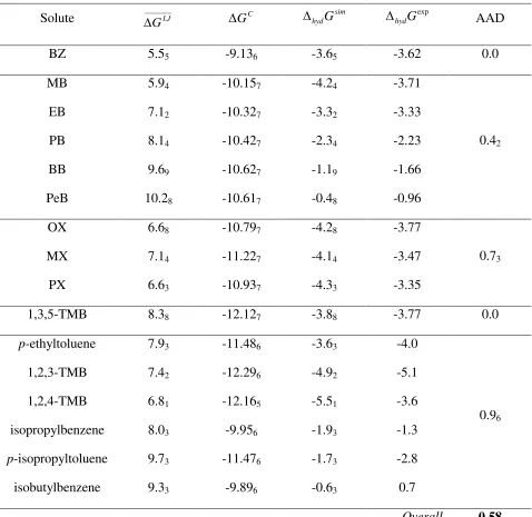
Table 4: LJ
(
LJ)
G∆ and electrostatic contributions (∆GC)to the predicted Gibbs
energy of hydration (∆hydGsim) of the full test and training sets. All data in kJ/mol. The subscripts give the statistical accuracy of the last decimal point shown.
Solute _______LJ G
∆ ∆GC ∆hydGsim
exp
G hyd
∆ AAD
BZ 5.55 -9.136 -3.65 -3.62 0.0
MB 5.94 -10.157 -4.24 -3.71
EB 7.12 -10.327 -3.32 -3.33
PB 8.14 -10.427 -2.34 -2.23
BB 9.69 -10.627 -1.19 -1.66
PeB 10.28 -10.617 -0.48 -0.96
0.42
OX 6.68 -10.797 -4.28 -3.77
MX 7.14 -11.227 -4.14 -3.47
PX 6.63 -10.937 -4.33 -3.35
0.73
1,3,5-TMB 8.38 -12.127 -3.88 -3.77 0.0
p-ethyltoluene 7.93 -11.486 -3.63 -4.0
1,2,3-TMB 7.42 -12.296 -4.92 -5.1
1,2,4-TMB 6.81 -12.165 -5.51 -3.6
isopropylbenzene 8.03 -9.956 -1.93 -1.3
p-isopropyltoluene 9.73 -11.476 -1.73 -2.8
isobutylbenzene 9.33 -9.896 -0.63 0.7
0.96
[image:31.595.82.560.185.650.2]Solute
Exp HydG ∆
→ Solute
(“Experimental”, Unpolarized, Gas) (“Experimental”, Polarized, Solvated)
G Sol G
∆ L
Pol G
∆
Solute
Exp SimG ∆
→ Solute
(“Model”, Polarized, Gas) (“Model”, Polarized, Solvated)
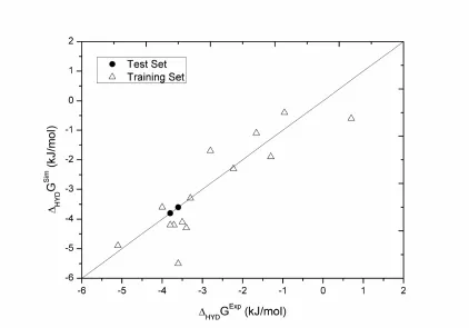
Figure 5: Comparison between experimental and predicted Gibbs energy of hydration
for all the compounds under study using the proposed new force field. Test set refers to
S1
Supporting Information:
Predicting Hydration Gibbs Energies of Alkyl-aromatics Using
Molecular Simulation: A Comparison of Current Force Fields and the
Development of a New Parameter Set for Accurate Solvation Data
Nuno M. Garrido1, Miguel Jorge1, António J. Queimada1, José R. B. Gomes2,
Ioannis G. Economou3 and Eugénia A. Macedo1,*
1. LSRE Laboratory of Separation and Reaction Engineering, Departamento de
Engenharia Química, Faculdade de Engenharia, Universidade do Porto, Rua do Dr.
Roberto Frias, 4200 - 465 Porto, Portugal
2. CICECO, Department of Chemistry, University of Aveiro, Campus Universitário de
Santiago, Aveiro 3810-193, Portugal
3. The Petroleum Institute, Department of Chemical Engineering, PO Box 2533, Abu
Dhabi, United Arab Emirates
*
S2
Table S1: LJ and electrostatic contributions to the predicted hydration Gibbs energies of benzene and linear alkylbenzenes using the TraPPE-UA force field. All data in kJ/mol. The subscripts give the statistical accuracy of the last decimal point shown. Abbreviations as detailed in the main manuscript.
Solute LJ
G
∆ C
G
∆ ∆hydGsim
exp
G hyd ∆
BZ 4.55 0 4.55 -3.62
MB 5.56 0 5.56 -3.71
EB 6.66 0 6.66 -3.33
PB 7.110 0 7.110 -2.23
BB 7.99 0 7.99 -1.66
PeB 9.16 0 9.16 -0.96
AAD 9.46
BZ* 5.55 -5.049 0.55 -3.62
AAD 4.2
[image:38.595.83.517.139.462.2]S3
Table S2: LJ and electrostatic contributions to the predicted hydration Gibbs energies
of benzene and linear alkylbenzenes using the OPLS-AA force field. All data in kJ/mol.
The subscripts give the statistical accuracy of the last decimal point shown.
Solute LJ
G
∆ C
G
∆ ∆hydGsim
exp
G hyd ∆
BZ 6.82 -8.21 -1.42 -3.62
MB 12.15 -12.248 -0.15 -3.71
EB 16.44 -11.708 4.74 -3.33
PB 19.44 -11.178 8.24 -2.23
BB 22.05 -11.188 10.85 -1.66
PeB 26.32 -11.098 15.22 -0.96
AAD 8.8 ± 4.9
Table S3: LJ and electrostatic contributions to the predicted hydration Gibbs energies
of benzene and linear alkylbenzenes using the Gromos-EH force field. All data in
kJ/mol. The subscripts give the statistical accuracy of the last decimal point shown.
Solute LJ
G
∆ C
G
∆ ∆hydGsim
exp
G hyd ∆
BZ 7.65 -12.668 -5.25 -3.62
MB 7.94 -9.237 -1.44 -3.71
EB 8.76 -9.537 -0.86 -3.33
PB 9.06 -9.447 -0.56 -2.23
BB 9.97 -9.547 0.37 -1.66
PeB 10.78 -9.497 1.28 -0.96
[image:39.595.83.517.476.703.2]S4
Table S4: LJ and electrostatic contributions to the predicted hydration Gibbs energies
of benzene and linear alkylbenzenes using the Gromos-UA force field. All data in
kJ/mol. The subscripts give the statistical accuracy of the last decimal point shown.
Solute LJ
G
∆ C
G
∆ ∆hydGsim
exp
G hyd ∆
BZ 1.76 0 1.76 -3.62
MB 2.53 0 2.53 -3.71
EB 3.33 0 3.33 -3.33
PB 4.03 0 4.03 -2.23
BB 4.18 0 4.18 -1.66
PeB 4.59 0 4.59 -0.96
S5
Tables S5-S12: CHelpG and NPA charges for the different molecules studied
• Table S5: Benzene (BZ)
Atom CHelpG NPA
C1 (4x) -0.062
C2 (2x) -0.103
-0.245
H1 (4x) 0.072
H2 (2x) 0.085
0.245
• Table S6: Toluene (MB)
1 2
3
4
5 6
7 8
9
10
11 12 13
14
15
Atom# CHelpG NPA Atom# CHelpG NPA Atom# CHelpG NPA
1 0.212 -0.042 6 -0.026 -0.238 11 0.072 0.245
2 -0.223 -0.709 7 -0.203 -0.241 12 0.098 0.240
3 -0.212 -0.240 8 0.109 0.240 13 0.066 0.245
4 -0.020 -0.238 9 0.069 0.245 14 0.059 0.252
S6
• Table S7: Ethylbenzene (EB)
1 2 3
4
5 6 7
8
9
10
11 12 13
14
15 16
17
18
Atom# CHelpG NPA Atom# CHelpG NPA Atom# CHelpG NPA
1 -0.167 -0.239 7 0.033 -0.488 13 -0.016 0.247
2 0.093 -0.036 8 0.105 0.240 14 0.164 -0.690
3 -0.167 -0.239 9 0.075 0.245 15 -0.016 0.246
4 -0.063 -0.239 10 0.080 0.245 16 -0.035 0.239
5 -0.096 -0.253 11 0.075 0.245 17 -0.054 0.239
S7
• Table S8: Propylbenzene (PB)
1 2 3
4
5 6 7
8
9
10
11 12 13
14
15 16
17 18
19 20
21
Atom# CHelpG NPA Atom# CHelpG NPA Atom# CHelpG NPA
1 -0.134 -0.239 8 0.099 0.240 15 0.022 0.245
2 0.096 -0.035 9 0.081 0.245 16 -0.137 -0.699
3 -0.134 -0.239 10 0.079 0.245 17 -0.144 0.239
4 -0.091 -0.239 11 0.080 0.245 18 -0.114 0.239
5 -0.079 -0.253 12 0.099 0.240 19 0.013 0.244
6 -0.091 -0.239 13 0.022 0.245 20 0.015 0.235
S8
• Table S9: Ortho-xylene (OX)
1
2 3 4
5 6 7
8
9
10
11 12
13 14
15
16 17
18
Atom# CHelpG NPA Atom# CHelpG NPA Atom# CHelpG NPA
1 -0.210 -0.233 7 -0.176 -0.708 13 0.051 0.247
2 -0.071 -0.247 8 -0.176 -0.708 14 0.054 0.249
3 -0.071 -0.247 9 0.114 0.239 15 0.054 0.249
4 -0.210 -0.233 10 0.077 0.244 16 0.051 0.247
5 0.106 -0.039 11 0.077 0.244 17 0.054 0.249
S9
• Table S10: Meta-xylene (MX)
1 2 3
4 5 6 7 8
9
10 11
12 13
14
15 16
17
18
Atom# CHelpG NPA Atom# CHelpG NPA Atom# CHelpG NPA
1 -0.247 -0.250 7 -0.149 -0.708 13 0.042 0.248
2 -0.009 -0.231 8 -0.130 -0.708 14 0.041 0.246
3 -0.250 -0.250 9 0.115 0.240 15 0.044 0.253
4 0.215 -0.035 10 0.074 0.244 16 0.035 0.247
5 -0.327 -0.237 11 0.115 0.240 17 0.040 0.253
S10
• Table S11: Para-xylene (PX)
1
2 3 4
5 6 7
8
9
10 11
12
13 14
15
16
17 18
Atom# CHelpG NPA Atom# CHelpG NPA Atom# CHelpG NPA
1 -0.173 -0.233 7 -0.172 -0.707 13 0.048 0.247
2 -0.179 -0.233 8 -0.165 -0.707 14 0.050 0.252
3 0.166 -0.051 9 0.105 0.239 15 0.048 0.247
4 -0.179 -0.233 10 0.106 0.239 16 0.046 0.247
5 -0.171 -0.233 11 0.106 0.239 17 0.049 0.252
S11
• Table S12: 1,3,5-Trimethylbenzene (TMB)
1 2 3 4 5
6 7
8 9
10
11 12
13 14 15
16
17 18
19
20
21
Atom# CHelpG NPA Atom# CHelpG NPA Atom# CHelpG NPA
1 -0.379 -0.245 8 -0.171 -0.707 15 0.042 0.250
2 0.263 -0.025 9 -0.184 -0.707 16 0.047 0.250
3 -0.379 -0.245 10 0.145 0.234 17 0.049 0.251
4 0.253 -0.025 11 0.146 0.234 18 0.046 0.244
5 -0.371 -0.245 12 0.142 0.234 19 0.050 0.244
6 0.256 -0.025 13 0.042 0.244 20 0.052 0.251
S12
Table S13: Prediction of liquid densities (g/l) at P = 1 bar using the new parameters set.
Solute T/K ρcalc AAD (%) T/K ρcalc AAD (%) T/K ρcalc AAD (%)
BZ 313 900.89 5.0 294 920.81 5.0 347 864.59 5.1
MB 311 873.63 2.5 293 891.78 2.6 345 840.36 2.5
EB 311 862.77 1.2 292 879.66 1.1 344 832.81 1.4
PB 309 861.21 1.4 291 876.55 1.3 343 832.87 1.6
BB 309 861.71 1.5 290 876.61 1.5 342 834.94 1.7
PeB 308 858.97 1.4 289 873.41 1.4 341 833.22 1.3
OX 309 879.67 1.5 291 896.16 1.6 343 850.61 1.4
MX 309 864.05 1.5 291 880.09 1.6 342 835.42 1.6
PX 309 860.23 1.5 291 875.86 1.5 342 831.99 1.6
TMB 308 874.50 2.4 289 889.19 2.3 340 847.92 2.6
S13
Table S14: Prediction of vaporization enthalpies (kJ/mol) at P = 1 bar using the new
parameters set.
Solute T/K ∆∆∆∆vapHexp EGas ELiq
sim vapH
∆ ∆∆ ∆
AAD
(kJ/mol)
BZ 313 33.0 102.4 69.1 35.9 2.9
MB 311 37.4 100.0 64.9 37.7 0.3
EB 311 41.5 121.8 83.8 40.6 1.0
PB 309 46.6 129.5 87.2 44.9 1.7
BB 309 49.9 137.9 91.0 49.5 0.4
PeB 308 54.8 145.9 94.9 53.7 1.2
OX 309 42.9 97.2 58.6 41.2 1.7
MX 309 42.2 97.2 59.1 40.6 1.6
PX 309 41.7 97.2 59.4 40.4 1.3
TMB 308 46.9 94.6 52.6 44.6 2.3
S14
Figure S1: Correlation between ∆GC (kJ/mol) and aromatic hydrogen point charges for BZ (the charge on the aromatic carbon is always symmetric to the hydrogen charge).
Figure S2: Correlations between C
G
∆ (kJ/mol) for TMB and different point charges on the substituted aromatic carbon atom (remaining charges are kept equal to their
[image:50.595.138.439.406.640.2]S15
Figure S3: Benzene liquid structure: computed Caro−Caro (aromatic carbon – aromatic
carbon), Haro −Haro (aromatic hydrogen – aromatic hydrogen) and Caro−Haro (aromatic carbon – aromatic hydrogen) radial distribution functions at 298 K using the
S16
Tutorial: How to assign charges for 1,2,4-TMB using the rule:
1) Assign each site (Carbon, Hydrogen or CHx) to its corresponding position in the
diagram of Figure 2.
2) For each site, determine the total number of substituents (Nj) on each position j (0 for
the current C/H atoms, 1 for C/H atoms in ortho position, 2 for C/H atoms in meta
position, and 3 for C/H atoms in para position). Recall that the maximum value of N is 1
for j=0,3 and 2 for j=1,2.
3) Compute the charge on each site by applying equation (4) and the charge increments
of Table 4.
The table below shows the number of substituents and the total charge on each site of
the 1,2,4-TMB molecule.
Atom N0 N1 N2 N3 q
C1 1 1 1 0 -0.1082
C2 1 1 0 1 -0.1160
C3 0 1 2 0 -0.1135
C4 0 1 1 1 -0.1213
C5 1 0 1 1 -0.1148
C6 0 2 1 0 -0.1147
CH7 1 1 1 0 0.1100
S17
H9 0 1 2 0 0.1193
H10 0 1 1 1 0.1195
CH11 1 0 1 1 0.1125
H12 0 2 1 0 0.117
0.0000
=
∑
Below are two examples of application of equation (4) to calculate the charge on the carbon atom at position 1 and on the CHx pseudo-atom at position 7.
Example:
1 0.1225 1* 0.0087 1* 0.0022 1* 0.0034 0 * 0.0044 0.1082
C
q = − + + + − = −
7 0.1225 1* 0.0096 1* 0.0026 1* 0.0003 0 * 0.0001 0.1100
CH