An analytical model for bore-driven run-up

Journal of Fluid Mechanics

Additional services for 

Journal of Fluid Mechanics:

Email alerts: Click here Subscriptions: Click here Commercial reprints: Click here Terms of use : Click here

An analytical model for bore­driven run­up

DAVID PRITCHARD, PAUL A. GUARD and TOM E. BALDOCK

Journal of Fluid Mechanics / Volume 610 / September 2008, pp 183 ­ 193 DOI: 10.1017/S0022112008002644, Published online: 08 August 2008

Link to this article: http://journals.cambridge.org/abstract_S0022112008002644

How to cite this article:

DAVID PRITCHARD, PAUL A. GUARD and TOM E. BALDOCK (2008). An analytical model for  bore­driven run­up. Journal of Fluid Mechanics, 610, pp 183­193 doi:10.1017/

S0022112008002644

Request Permissions : Click here

doi:10.1017/S0022112008002644 Printed in the United Kingdom

An analytical model for bore-driven run-up

D A V I D P R I T C H A R D1, P A U L A. G U A R D2

A N D T O M E. B A L D O C K2

1 _{Department of Mathematics, University of Strathclyde, 26 Richmond St, Glasgow G1 1XH, UK}

[email protected]

2_{Department of Civil Engineering, University of Queensland, St Lucia, Queensland 4072, Australia}

(Received4 March 2008 and in revised form 9 June 2008)

We use a hodograph transformation and a boundary integral method to derive a new analytical solution to the shallow-water equations describing bore-generated run-up on a plane beach. This analytical solution differs from the classical Shen–Meyer runup solution in giving significantly deeper and less asymmetric swash flows, and also by predicting the inception of a secondary bore in both the backwash and the uprush in long surf. We suggest that this solution provides a significantly improved model for flows including swash events and the run-up following breaking tsunamis.

1. Introduction

The behaviour of waves as they run up on the shore is of great practical and scientific interest. Important contexts include beach morphodynamics (e.g. Pritchard & Hogg 2005), waves overtopping breakwaters (e.g. Peregrine & Williams 2001) and the run-up of tsunamis when the wave breaks offshore (e.g. Guard, Baldock & Nielsen 2005). Such problems are often tackled through detailed numerical simulation, but an important role continues to be played by exact and asymptotic analyses which provide a baseline for numerical studies and which permit detailed investigation of the flow behaviour.

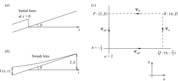
In this study we consider the particular case of the flow which results after an incoming bore has collapsed, driving a thin tongue of water up the beach (figure 1a, b). The most significant analytical work is due to Shen & Meyer (1963, hereafter referred to as SM63). Two features of their analysis are particularly significant. First, they obtained an asymptotic description of the flow, valid under very general conditions on the incoming wave; this description may be interpreted as a simple-wave solution to the shallow-water equations, and has been employed as an analytical model of flow in a swash lens (e.g. Peregrine & Williams 2001). Second, they predicted the breakdown of solutions during the backwash: this breakdown was later verified by the numerical simulations of Hibberd & Peregrine (1979), and is associated with the ince-ption of a receding ‘backwash bore’. The backwash bore occurs neither in the SM63 solution nor, as far as we are aware, in any existing analytical solution for wave run-up.

Initial bore

(a) (c)

(b)

Swash lens

2 A at x = 0

θ

θ

x

b

a

x

h (x, t)

P : (2, β) R : (α, β)

a= 2

6b

6ab

6a 6ab

b = –2 3

Q : (α, – )2₃

Figure 1.(a,b) Sketches of the solution _h(_{x, t}) at (a)_t = 0, the moment of collapse of the initial bore and (b) the maximum run-up of the swash; dimensional variables are used. (c) Schematic of the contour of integration in the (a, b)-plane for the boundary-integral method.

& Baldock (2007, hereafter referred to as GB07), obtained numerical results for swash flow using a characteristic-tracking method, with a boundary condition defined on a receding characteristic, and demonstrated that these accorded much better with laboratory measurements than the SM63 solution (see figure 4 below).

This study presents an analytical solution for run-up and swash driven by the same boundary conditions as in GB07. This solution is expressed in terms of hodograph variables, and so must be numerically mapped back to physical coordinates; nevertheless, the analytical solution has several advantages over a purely numerical one. Because it allows information to be obtained at a particular point without computing the rest of the solution, it allows more thorough investigation of details of the flow; it also permits direct evaluation of the locations where breakdown of the solution occurs. Finally, the analytical model permits Lagrangian approaches to the sediment transport problem, which have been productive in similar contexts (e.g. Pritchard & Hogg 2005): we will not discuss sediment transport here, but it remains an additional motivation for this work.

2. Mathematical development of the model

2.1. Governing equations and boundary conditions

The one-dimensional shallow-water equations for flow over a plane beach, with the sea to the left, are given in non-dimensional form by

∂h ∂t +u

∂h ∂x +h

∂u ∂x = 0,

∂u ∂t +u

∂u ∂x +

∂h

∂x + 1 = 0. (2.1)

2004): this will be the case as long ascd tanθ, wherecd is a Chezy drag coefficient. Equations (2.1) can be written in characteristic form as

dα

dt = 0 on dx

dt =u+c= 1

4(3α+β)−t, dβ

dt = 0 on dx

dt =u−c= 1

4(α+3β)−t, (2.2) where the characteristic quantities are defined as

α=u+ 2c+t, β=u−2c+t, c=√h. (2.3)

2.1.1. The Shen–Meyer (1963) solution

The solution obtained by SM63 as an asymptotic result, valid in a region of the characteristic plane close to the singular point which corresponds to the shoreline, and presented as an exact solution by Peregrine & Williams (2001), is given by

h(x, t) = 1 9

2−1 2t−

x t

2

, u(x, t) = 2 3

1−t+x t

. (2.4)

This solution represents a simple wave: all incoming characteristics from the left carry α = 2, while allβ-characteristics originate from (0,0), the shoreline at the instant of bore collapse (figure 1a). The moving shoreline is located at xsh(t) = 2t − 1₂t2, and corresponds toα=β= 2; equations 2.4 are valid only in x < xsh(t).

2.1.2. Boundary conditions

A variety of boundary conditions may be imposed upon the shallow-water equations. Equations (2.4) may be treated as solving an initial-value problem ana-logous to the dam-break problem (Ritter 1892); alternatively, they can be thought of as a simple wave with incoming characteristic information α = 2, and this suggests that it is natural to specify seaward conditions in terms of incoming characteristic information. Precisely how this information is specified is largely a matter of convenience. When the plane beach is regarded as part of a more complex bathymetry, it is convenient to supply boundary data at some fixed spatial position (cf. Guardet al.2005). When working with the characteristic equations (2.2), however, it is more convenient to specify incoming α-values along a β-characteristic (GB07), giving the solutions obtained below a particularly tractable form. We will therefore consider only boundary conditions imposed in this way, though we will investigate how they may be related to spatially fixed conditions.

2.2. Solution method

Rewriting the characteristic equations with (α, β) as the independent variables gives

∂x ∂β =

1

4(3α+β)−t

∂t ∂β, ∂x ∂α = 1

4(α+ 3β)−t

∂t

∂α. (2.5)

Differentiating these equations by α and by β respectively then eliminating x, we obtain

∂2t ∂α∂β =

3 2(α−β)

∂t ∂α − ∂t ∂β . (2.6)

Note that this equation, with differently defined α andβ, can also be obtained from a hodograph transformation of the SWEs over a horizontal bed (Hogg 2006), so the solutions obtained below may be reinterpreted as modified dam-break flows.

mapping (α, β)→(a, b)), then by Stokes’s theorem we have the identity

∂_D

(Udb−Vda) = 0, (2.7)

where the boundary∂Dis traversed in an anticlockwise sense. In (2.7), we define

U =− 3

2(a−b)tB+ 1 2

∂t ∂bB−

1 2t

∂B

∂b, V = 3

2(a−b)tB+ 1 2

∂t ∂aB−

1 2t

∂B

∂a, (2.8)

where we considert as a function of (a, b), and where

B(a, b;α, β) = (a−b) 3

(a−β)3/2_(α−_b)3/2F

3 2,

3 2; 1;

(a−α)(β−b) (a−β)(α−b)

(2.9)

(Garabedian 1964, p. 150). HereF is a hypergeometric function. Note in particular thatB is constructed such that

∂B ∂b =−

3B

2(a−b) on a=α;

∂B ∂a =

3B

2(a−b) on b=β; B(α, β;α, β) = 1. (2.10) Assume that we knowt(α, β) on some curveCin the (α, β)-plane (figure 1c). For a point (α, β) within the domain of dependence of this curve, we choose∂Dto comprise Cb (a section of the lineb=β joiningCto the pointR: (a, b) = (α, β)),Ca (a section of the linea = α joining C to the point R), and Cab (the portion of C between the intersections withCa andCb). We now have

Cab

(Udb−Vda) +

Ca 1 2t ∂B ∂b + 1 2B ∂t ∂b db− Cb 1 2t ∂B ∂a + 1 2B ∂t ∂a

da= 0, (2.11)

where we have used the boundary conditions onB onCb andCa. Defining P to be the point whereCb intersectsCand Qto be the point whereCa intersectsC, we can then write

t(α, β) = 1

2[t(Q)B(Q;α, β) +t(P)B(P;α, β)]−

Cab

(Udb−Vda). (2.12)

To proceed, we must specify the boundary conditions for bore-driven run-up or swash.

2.3. Bore-driven run-up: the general case

The solutions of GB07 are constructed assuming that all β-characteristics fan out from (x, t) = (0,0) as in the classic solution of SM63, while the flow is ‘fed’ by incoming α-characteristics which, when they cross the characteristic β=−2/3, are carrying the valueα= 2 +kt for some constant k. (This particularβ-characteristic is chosen because it is tangent att= 0 to the linex= 0; the linear dependence on t is assumed for simplicity.) The latter condition may be simply written ast= (α−2)/k on β=−2/3; a little consideration indicates that the former may be represented as t= 0 on α= 2, for valuesβ <2. (The point (α, β) = (2,2) corresponds to the moving shoreline, so the solution is degenerate here.) The curve C therefore comprises the straight line α= 2 for −2/3< β together with the straight line β=−2/3 for 2< α (see figure 1c).

We then haveP : (2, β) andQ: (α, β0), and we may write

Cab

(Udb−Vda) =

a=2, b=β0

a=2, b=β

Udb−

b=β0, a=α

b=β0, a=2

Vda=−

b=β0, a=α

b=β0, a=2

Vda (2.13)

sincet = 0 and∂t/∂b= 0 on the curvea= 2. It follows that

t(α, β) = 1

2[t(α, β0)B(α, β0) +t(2, β)B(2, β)]

+

α

2

3B(a, β0)f(a) 2 (a−β0)

+B(a, β0)

2 f

_(a)−f(a)

2 ∂B ∂a

(a,β0)

da, (2.14)

where B(a, b) ≡ B(a, b;α, β) tacitly. Integrating by parts and using the boundary values oft and B and the conditionf(2) = 0, we obtain

t(α, β) =

α

2

B(a, β0)

3 2

f(a) (a−β0)

+f(a)

da. (2.15)

Once we have obtained t(α, β), we require only to obtain x(α, β) to have specified the solution entirely. This can be done simply by integrating along aβ-characteristic, recalling that these all originate from (x, t) = (0,0). Integrating equation (2.5b) yields

x(α, β) =

α 4 + 3 4β

t(α, β)−1

2(t(α, β)) 2₋ 1

4

α

2

t(α, β) dα. (2.16)

Although there does not appear to be a convenient further simplification of the solutions, this form is straightforward to evaluate and to work with.

In the particular case of the GB07 solutions, we haveβ=−2/3 andf(a) = (a−2)/k; substituting these into equation (2.15) yields

t(α, β) = 1 k

α

2

5a−14₃ 2a+ 2

3

Ba,−2₃;α, βda. (2.17)

The results presented here were obtained by integrating (2.17) numerically in Maple to obtain an array of values of t(α, β), and obtaining x(α, β) from this through quadrature along β-characteristics.

3. Results

3.1. Hydrodynamics

0 0.5 1.0

x x

1.5 2.00 1 2 3 4

(a) (b)

t

0 0.5 1.0 1.5 2.00 1 2 3 4

Figure 2.Solutions for (a)k= 0.5; (b)k= 1. In each case, solid lines are contours of velocity

u(x, t) at intervals of 0.2 (theu= 0 contour is easily identified as that which meets the shoreline att= 2), while dashed lines are contours of depthh(x, t) at intervals of 0.1.

–2.0 –1.6

u(x; t) h(x; t) –1.2

(a) (b)

–0.2 0 0.2

x x

0.4 0.6 0.8

0 0.1 0.2

–0.2 0 0.2 0.4 0.6 0.8

Figure 3.‘Snapshots’ of the hydrodynamic variables for k= 1, late in the backwash: variables are shown at t= 3.5, 3.75 and 3.875 (solid lines); dotted lines show the SM63 solution.

0.1 0.2 h (t; x)

0.3 0.4

0 0.5 1.0 1.5 2.0 t

2.5 3.0 3.5 4.0

Figure 4.Modelled and experimental fluid depths, replotted from GB07, figure 12. Data are measured atx= 0.2 (+),x= 0.3 (×) andx= 0.4 (∗); lines are SM63 solution (solid) and new solution withk= 1 (dashed), at the same locations (highest linesx= 0.2; lowest x= 0.4).

2.0 2.4 2.8 3.2 3.6

0 1 2 3 4

α (t; 0)

t

–0.3 –0.2 –0.1 0 q (t; 0)

0.1 0.2 0.3 (b) (a)

0 1 2

t

3 4

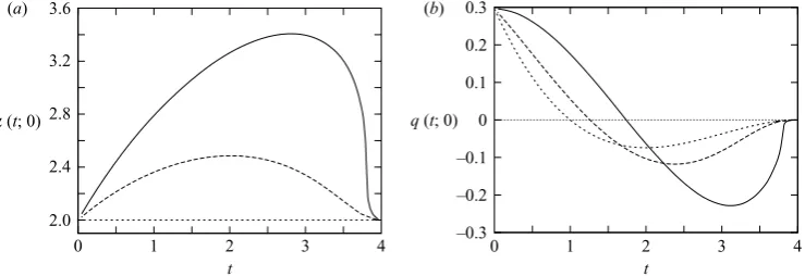
Figure 5. Behaviour of the solution along the line_x= 0, for_k= 1 (solid lines),_k= 0_.5 (heavy dashed lines) andk= 0 (SM63; light dashed lines): (a) values of the incoming characteristic quantityα; (b) flux of fluidq=uhacrossx= 0.

3.2. Behaviour atx= 0

An alternative to specifying incoming characteristic information on a particular β-characteristic is to specify it at some fixed satial position such as the original shoreline x= 0 (see e.g. Guard et al. 2005). In principle, any reasonable variation of α atx= 0 could be represented using (2.15) with appropriate choices of β0 andf(α); in practice, choosing these would require a rather cumbersome iterative process which would obviate most of the benefits of the simple analytical solution. It is, however, worth considering how the results presented here relate to those which would be obtained imposing a spatially fixed boundary condition atx= 0.

The incoming characteristic informationαatx= 0 is plotted againsttin figure 5(a). For small values of t, αx=0 ∼2 +kt, but it deviates from this as t increases and the β = −2/3 characteristic retreats further offshore. Towards the end of the swash event, αx=0 decreases sharply, as the flow becomes supercritical and offshore, and α-characteristics carrying lower values ofα start to propagate out of the domain. For k . 1, a smooth variation of α at the boundary results; for k = 1, where solution breakdown occurs just offshore, the variation towards the end of the swash is very sharp indeed, while for larger values of k (not shown here) the line of solution breakdown crossesx = 0 andα varies discontinuously. In the numerical simulations of Hibberd & Peregrine (1979) and some of those of Guardet al.(2005),αx=0is forced to increase throughout the period of inundation, and since this is inconsistent with the shoreline valueα = 2 at t = 4, the solution must become discontinuous at some point within the swash zonex >0. In our solutions, it is possible for the solution to remain continuous throughout the swash zone, at least fork.1. Behaviour at larger values is discussed below.

–1.0 –0.5 0 0.5 1.0

2.0 2.5 3.0 3.5 4.01.8 1.85 1.90

β

(a)

1.95 2.00

1.0 1.2 1.4 1.6 x t

α

1.8 2.00.5 1.0 1.5 2.0 2.5 3.0 3.5 (b)

Figure 6.(a) The JacobianJ(α, β), with the contourJ = 0 (solid line). The quantity plotted is tanh(J) rather thanJ itself, so the entire range ofJ from −∞to ∞is included in a finite scale: breakdown corresponds to tanh(J) = 0 or tanh(J)→ ±1. (b) Selectedβ-characteristics of the solution withk= 2, together with the breakdown line: solid lines areβ-characteristics; the dashed line represents the breakdown line while the dotted line represents the shoreline.

3.3. Breakdown of the solutions: inception of a backwash bore

An advantage of the analytical solution is that it is possible to identify the locations where the solution, considered in the (x, t)-plane, breaks down. Solution breakdown occurs where characteristics cross, and may be tentatively identified with bore inception; more formally it indicates the loss of validity of the shallow-water equations. It corresponds to the conditionJ = 0 orJ → ±∞, where

J = ∂x ∂α

∂t ∂β −

∂x ∂β

∂t ∂α =

(β−α) 2

∂t ∂α

∂t

∂β (3.1)

is the Jacobian of the transformation from (x, t) to (α, β) coordinates. The Jacobian may be evaluated straightforwardly: writing the integrand in (2.15) as g(a, α, β), we have

∂t ∂α =

α

2 ∂g

∂α(a, α, β)da+g(α, α, β) and ∂t ∂β =

α

2 ∂g

∂β(a, α, β) da. (3.2)

These integrals may readily be evaluated along witht(α, β), using Maple as described above. It is worth noting that J(α, β) is strictly proportional to k−2: this reflects the fact that in the limit k → 0 the solution approaches a simple wave in which the hodograph transformation breaks down everywhere.

0 1 2 t(T)

u(T)

x x(T)

3 4

(a) (b)

1.0 1.5 2.0 2.5 3.0

x –2

–1 0 1

1.0 1.5 2.0 2.5 3.0

Figure 7. Properties of the solution at the pointT where breakdown first occurs. (a) Location

x(T) (solid line) and timet(T) (dashed line) of breakdown. (b) Velocity u(T) at the point of first breakdown.

Figure 6(b) illustrates the relationship between the breakdown line and the β-characteristics for the case k= 2, for which breakdown occurs well within the region x >0. Characteristics withβ > βT meet the breakdown line while travelling seawards: on these characteristicsJ = 0 at the breakdown line, so they start to double back on themselves here. Meanwhile, β-characteristics withβ < βT approach the breakdown line from the seaward side, but do not encounter J = 0 at this point: as far as they ‘know’, they can simply continue into the area landwards of the breakdown line. In a full solution, the different hydrodynamic information being carried by the high-β and low-βcharacteristics is reconciled across a discontinuity (a ‘secondary’ bore). The trajectory of this bore must be calculated separately (cf. §4 of Hogg 2006): for the moment we merely note that because a bore must be fed by characteristic information from either side, and because information carried by high-β characteristics cannot propagate seawards past the breakdown line, the breakdown line marks the seaward limit of the possible position of the bore. Consequently, that part of the solution seaward of the breakdown line can be regarded as reliable no matter what occurs landward of it.

Figure 7(a) shows how the position of the point in (x, t) space corresponding toT, at which the bore first forms, varies with k. For higher k, the solution breaks down earlier; the spatial position of bore formation enters the region x > 0 for k ≈ 1.02, increases to a maximum of about x(T)≈ 1.82 fork ≈2.04 and then decreases with increasing k. Because the secondary bore first appears at the pointT in (α, β)-space, which is independent of k, the depth of the fluid where the bore is first formed is a constant, h(T)≈ 0.017. The velocity of the fluid at the point when the bore first occurs, however, does depend onk (figure 7b). It is particularly noteworthy that for values of k &1.83, the secondary bore first forms when u(T)>0, so it is actually a feature of the uprush rather than the backwash.

4. Conclusions

We have presented a new class of solutions to the shallow-water equations over a plane beach, which may be regarded as analytical models of the swash flow generated by a bore approaching the shore. These solutions are in agreement with the numerical results of Guard & Baldock (2007), and thus agree significantly better with laboratory measurements of swash flows than does the classic solution due to Shen & Meyer (1963). An interesting feature of the new solutions is that, in accordance with earlier predictions and numerical results Hibberd & Peregrine (1979), they include the inception of a secondary bore when the shallow-water solution breaks down. The location of the initial breakdown may easily be calculated using the analytical solution, and it is found that for swash supplied with sufficiently strongly increasing incoming characteristic information, the breakdown and bore inception may even occur during run-up rather than during backwash. This indicates the possibility of a secondary bore forming during the run-up of long surf. The thorough investigation of the secondary bore may be a worthwhile direction for future work within the framework employed here.

As with other exact solutions to the shallow-water equations, our analytical model provides a benchmark for numerical integration methods. Another possible application is as the hydrodynamic component in a semi-analytical description of suspended sediment transport in the swash zone or under tsunami run-up (cf. Pritchard & Hogg 2005; Pritchard & Dickinson 2008). Likewise, it would be interesting to investigate the transport of boulders and cobbles under this ‘modified’ swash flow (cf. Luccioet al.1998) and to employ it to estimate the destructive capabilities of tsunami waves (cf. Yeh 2006). Finally, it would be useful to investigate the interaction of the inviscid solution obtained here with a frictionally affected ‘tip’ very close to the swash front, following analogous work on dam-break flow by Hogg & Pritchard (2004).

D. P. acknowledges the support of a University of Strathclyde Faculty of Science Starter Grant (ref. VA5525C), and thanks Dr Andrew J. Hogg for introducing him to the boundary-integral method. P. A. G. acknowledges the support of an Australian Postgraduate Award from the Australian Government. This work was also supported by the Australian Research Council (project DP0877235). We thank three anonymous referees for their very constructive comments.

R E F E R E N C E S

Baldock, T. E., Hughes, M. G., Day, K. & Louys, J. 2005 Swash overtopping and sediment

overwash on a truncated beach.Coastal Engng 52, 633–645.

Baldock, T. E., Kudo, A., Guard, P. A., Alsina, J. M. & Barnes, M. P. _{2008 Lagrangian}

measurements and modelling of fluid advection in the inner surf and swash zones.Coastal EngngDoi:10.1016/j.coastaleng.2008.02.013.

Garabedian, P. R.1964Partial Differential Equations. Wiley.

Guard, P. A. & Baldock, T. E.2007 The influence of seaward boundary conditions on swash zone

hydrodynamics.Coastal Engng 54, 321–331.

Guard, P. A., Baldock, T. & Nielsen, P.2005 General solutions for the initial run-up of a breaking

tsunami front. InIntl Symp. on Disaster Relief on Coasts. Monash University, Australia.

Hibberd, S. & Peregrine, D. H.1979 Surf and run-up on a beach: a uniform bore.J. Fluid Mech.

95, 323–345.

Hogg, A. J.2006 Lock-release gravity currents and dam-break flows.J. Fluid Mech.569, 61–87. Hogg, A. J. & Pritchard, D. 2004 The effects of hydraulic resistance on dam-break and other

Luccio, P. A., Voropayev, S. I., Fernando, H. J. S., Boyer, D. L. & Houston, W. N.1998 The

motion of cobbles in the swash zone on an impermeable slope.Coastal Engng 33, 41–60.

Peregrine, D. H. & Williams, S. M. 2001 Swash overtopping a truncated plane beach.J. Fluid

Mech.440, 391–399.

Pritchard, D. & Dickinson, L.2008 Modelling the sedimentary signature of long waves on coasts:

implications for tsunami reconstruction.Sed. Geol.206, 42–57.

Pritchard, D. & Hogg, A. J.2005 On the transport of suspended sediment by a swash event on a

plane beach.Coastal Engng52, 1–23.

Ritter, A.1892 Die Fortpflanzung der Wasserwellen.Z. Vereines Deutsch. Ing.36(33), 947–954. Shen, M. C. & Meyer, R. E.1963 Climb of a bore on a beach. Part 3. Run-up.J. Fluid Mech.16,

113–125.

Yeh, H. 2006 Maximum fluid forces in the tsunami runup zone.J. Waterway Port Coastal Ocean