for assessing the appropriateness of a fluid description at the continuum level by utilizing kinetic information rather than macroscopic flow quantities alone. We propose a new kinetic criterion to indirectly assess the errors introduced by a continuum-level description of the gas flow. The analysis, which includes numerical demonstrations, focuses on the validity of the Navier-Stokes-Fourier equations and corresponding kinetic models and reveals that the new criterion can consistently indicate the validity of continuum-level modeling in both low-speed and high-speed flows at different Knudsen numbers.
DOI:10.1103/PhysRevE.89.063305 PACS number(s): 47.11.−j,47.45.−n,47.61.−k
I. INTRODUCTION
In microelectromechanical systems (MEMS) that depend on gas flows, there may be coexisting continuum-fluid and highly rarefied regions [1]. To qualitatively identify the rar-efaction level of the local flowfield, the Knudsen number (Kn) is often used, which is the ratio of the mean free path of gas molecules to a characteristic length scale of the flow process. It is commonly accepted that the conventional hydrodynamic description is only valid for Kn<0.001. When Kn is larger than 0.001, rarefaction effects have to be taken into account. Rarefied flows can be further classified into the slip (0.001 Kn0.1), transitional (0.1Kn10), and free molecular (Kn10) flow regimes.
Multiscale methods are needed when gas flows have a broad range of rarefaction levels (see, for example, Refs. [2–15], and references therein). The conventional Navier-Stokes-Fourier (NSF) equations are computationally efficient but are only valid in the hydrodynamic regime. Although their capabilities may be extended into the slip flow regime by applying appropriate velocity-slip and temperature-jump boundary con-ditions, their applicability range is strictly limited. By contrast, accurate kinetic gas solvers, including the direct simulation Monte Carlo (DSMC) method [16] and direct solution of the Boltzmann equation [17], can be computationally very ex-pensive. Therefore, to strike a balance between computational costs and simulation accuracy, multiscale schemes are being developed that take advantage of both kinetic and continuum-fluid solvers, i.e., deploying a kinetic solver only in the rarefied flow regions and a continuum solver in the hydrodynamic regions. The two types of method are coupled together by exchanging information at interfaces where they overlap.
*[email protected] †[email protected] ‡[email protected]
§To whom the correspondence should be addressed: yonghao.
However, it has not proven easy to exchange information between two methods with different theoretical frameworks. It is problematic for the continuum solver to recover the accurate information required by the kinetic method [12]. Although the kinetic model can provide the information necessary for the continuum model, it can be computationally expensive [4]. The statistical noise associated with particle methods may also affect the accuracy and stability of the hybrid solver [12].
Recently, several new multiscale schemes have been con-structed purely on the basis of gas kinetic theory [18–21]; we call these kinetic multiscale schemes (KMS) here. A distinctive feature of KMS is that the same evolutional quantity (i.e., the molecular velocity distribution function) is used to describe flowfields with different rarefaction levels, leading to relatively easy information exchange at the model coupling interfaces [19,20]. To capture different levels of rarefaction, usually different discrete velocity sets are necessary. In general, more discrete velocities are needed for higher levels of rarefaction, and fewer discrete velocities are required for lower levels of rarefaction. In particular, there have been efforts to design schemes specialized in continuum-level modeling, e.g., the gas-kinetic Bhatnagar-Gross-Krook (BGK) Burnett solutions [22]. This provides a good opportunity to improve the efficiency of multiscale solvers. It is important practically to use fewer discrete velocities, or specialized continuum-level solvers, as widely as possible in the flow field wherever they are valid.
FIG. 1. (Color online) Cross-channel profiles of (left) the entropy generation rate [28] and (right) parameter B [26] for low-Mach-number planar Couette flows. The flows are solved with the linearized-BGK equation by using Gauss-Hermite quadrature. The Mach number is defined as Ma=Uw/
√
RT0and the Knudsen number is Kn=
√
π/2[μ0
√
RT0/(P0L)] (see Sec.III). The planar channel walls are at [−0.5, 0.5].
information exchange between the region can be accomplished by using simple interpolation and extrapolation operations.
An appropriate equilibrium breakdown parameter plays a key role in the success of any multiscale scheme, such as KMS. In order to couple kinetic methods and continuum-fluid solvers together, a breakdown parameter is required to determine where and when to switch between the two types of model. As a continuum model is not valid for highly rarefied flows, it is necessary to assess the modeling error introduced whenever it is applied. For simulation efficiency, the continuum solver should be deployed in the flowfield as widely as possible as long as it satisfies the requirement for solution accuracy. For KMS, a continuum-fluid model breakdown parameter is still of key importance. If a computational region is known to be solvable by the NSF equations, optimized kinetic solvers can be used to achieve better efficiency as discussed above, e.g., the nine lattice velocity model.
Various breakdown parameters have been proposed in the literature. The global Knudsen number has often been used [2]. Other parameters are also suggested, such as Tsien’s parameter [23], Bird’s parameterP [24], the local Knudsen number [13,14], Tiwari’s criterion [25], the parameterB[26], the criterion proposed by Lockerby et al. [2], and some others [27,28]. Although these breakdown parameters have had some success, in particular, for high-speed flows, it is fair
to say that there is no general parameter available. It remains an open research question to identify a general continuum model breakdown parameter for quantifying modeling accuracy. In particular, most of the available parameters are based on macroscopic quantities, which does not take advantage of the kinetic level information available in KMS.
Our aim here is to devise new breakdown param-eters for KMS. The central idea is to make best use of the kinetic level information in KMS provided by the molecular velocity distribution function (from which the relevant macroscopic quantities can also be obtained). The resulting parameters should not solely depend on macroscopic flow properties, unlike other available parameters.
II. CONTINUUM MODEL BREAKDOWN
The development of previous continuum model breakdown parameters has been based on the Boltzmann equation and its asymptotic solution [29]. The Boltzmann equation describes the dynamical behavior of dilute gases, under the assumptions of binary collisions between gas molecules and of molecular chaos. A single molecular velocity distribution function describes the gas motion.
Various series solution methods have been used to tackle the Boltzmann equation. Among them, the Chapman-Enskog
FIG. 2. (Color online) Cross-channel profiles ofEeq
[image:2.608.116.493.74.212.2] [image:2.608.113.491.582.720.2]FIG. 3. (Color online) Cross-channel profiles ofEeq
s (left) andE
NSF
c (right) for linear Couette flows at Kn=0.1. The planar channel walls are at [−0.5,0.5].
expansion [29] is widely used to approximate the distribution function as
f =f(0)+f(1)+f(2)+ · · · +f(α)+ · · ·, (1)
where the distribution functionsf(α)in increasing orders in Kn can be obtained from the Boltzmann equation. The Maxwell-Boltzmann equilibrium distribution,
feq= ρ
(2π RT)3/2 exp
− ς2
2RT
, (2)
is the zeroth-order solution f(0) and leads to the Euler hydrodynamic equations. Here,ρ denotes the gas density;T
the temperature;Rthe gas constant;ςthe peculiar velocity of molecules (which isξ −u, whereξ represents the molecular velocity); anduis the macroscopic fluid velocity.
In Eq. (1),f(1)provides a nonequilibrium correction of the order of the small parameter Kn. The NSF-level estimation for
f(1)is
f(1)≈fNSF≈feq
σijς<iςj > 2pRT
+ 2qiςi 5pRT
ς2
2RT −
5 2
,
(3)
wherep is the gas pressure, and the shear stressσij and the heat fluxqiare related to the following first-order gradients of
velocity and temperature:
σij = −2μ
∂u<i
∂xj >
, qi= −κ
∂T ∂xi
, (4)
whereμandκ denote the viscosity and thermal conductivity. Here we only keep the first-order Sonine expansion term, which is exact for Mawellian gases (see, e.g., Refs. [29,30] for detail); however, this is expected to be sufficient for our purpose. In fact, at the core of KMS is often an appropriate kinetic model equation (e.g., the BGK model) rather than the Boltzmann equation, which provides information of NSF-level accuracy at the first order of the Sonine expansion.
Following the same principle, we can obtainα-order (with respect to small Kn) corrections to the equilibrium distribution function. So higher-order hydrodynamic equations can be derived, e.g., the Burnett and super Burnett equations. As an alternative to the Chapman-Enskog expansion, the moment method provides a different way of solving the Boltzmann equation and leads to a number of extended hydrodynamic models, e.g., Grad-13 [31], R13 [32], R26 [33]. Therefore, regarding a continuum-fluid model breakdown parameter, we need to keep in mind which set of hydrodynamic equations or what order kinetic model are used [34].
As the NSF equations or NSF-level kinetic models are used by most multiscale methods we will focus on this continuum model. Also, since the applicability of the continuum fluid model has been effectively extended well beyond the NSF
FIG. 4. (Color online) Cross-channel profiles ofEeq
[image:3.608.120.489.73.211.2] [image:3.608.114.489.584.720.2]FIG. 5. (Color online) Cross-channel comparison ofEeq
s (left) andE
NSF
c (right) for linear Couette flows at Kn=0.01 and Kn=1 for small Mach numbers. The planar channel walls are at [−0.5,0.5].
equations [30], hereafter, “continuum breakdown” refers to the failure of the NSF equations, or the NSF-order kinetic model.
To establish a continuum breakdown parameter, and taking our lead from the Chapman-Enskog expansion, we separate the distribution function into three parts, i.e.,feq,fNSF, and
fH as
f =feq+fNSF+fH, (5)
wherefH represents all higher-order nonequilibrium correc-tions. From the Chapman-Enskog expansion, we can usefNSF from Eq. (3) to recover the NSF model. The higher-order correctionsfH produce the Burnett equations and beyond.
Therefore, we may directly use the information provided by
feq,fNSF, andfHto assess the validity of the NSF equations and an NSF-order kinetic model. For assessing other high-order models, such as the Burnett equations and the R13 model,
fH needs to be split further.
The Chapman-Enskog expansion indicates that there are various levels of nonequilibrium corrections to the equilibrium distribution function. As “nonequilibrium” is a very broadly used term, in this paper we equate the level of nonequilibrium to how far the molecular velocity distribution function deviates from the local Maxwellian equilibrium distribution. So the Euler equations are the continuum model for describing locally equilibrium flows, and the NSF equations provide a first-order nonequilibrium correction. A comparison of f −feq tofeq indicates the deviation from equilibrium, and hence
indirectly assesses whether the Euler equations are a valid model or not. When we examine the validity of the NSF equations and an NSF-order kinetic model, we may indirectly evaluate fNSF and fH, then for the NSF equations to be sufficiently accurate,fNSFshould be significantly larger than
fH so that the high-order corrections can be neglected. Many previous breakdown parameters were based on comparing nonequilibrium corrections with the equilibrium component, which is more appropriate for examining the validity of the Euler equations than the NSF equations.
Let us consider simple linear cases, where the leading order of feq is O(1), while that of fNSF can be represented by the shear stress term∼μ∂u<i/∂xj >, which isO(MaKn), cf. Eq. (3). Therefore, as a breakdown parameter, using either
fNSF itself or a ratio ∼fNSF/feq will lead to be the order O(MaKn). Here Ma is the Mach number, which is defined as the ratio of characteristic speed to the sound speed (see, e.g., Sec.III for the definition for Couette flows). However, for a linear flow condition the Mach number is not relevant to the validity of the NSF equations. This can be confirmed through numerical simulations of simple Couette flow, as shown in Fig.1, where two parameters are evaluated, namely, the entropy generation rate from Ref. [28] and the parameter B from Ref. [26]. For kinetic model equations, the entropy generation rate can be calculated as 1τ(feq−f) logf dξ, where τ is the relaxation time. The parameter B depends on macroscopic quantities, i.e., B =max(|σij|,|qi|). As can be seen in Fig. 1 both parameters fail to perform well as
FIG. 6. (Color online) Half-channel profiles ofEeq
s andE
NSF
[image:4.608.114.490.75.212.2] [image:4.608.116.492.593.733.2]FIG. 7. (Color online) Half-channel profiles ofEeq
s andE
NSF
c for nonlinear Couette flows at Kn=0.1. breakdown parameters for the NSF equations: both the entropy
generation rate and parameter B are significantly smaller for larger Knudsen number (Kn=1.0), where the NSF equations are not valid, than for smaller Knudsen number (Kn=0.01), where the NSF equations may be applicable with velocity-slip and temperature-jump boundary conditions.
It is also interesting to estimate the order of the ratio of
fNSFtofH. For this purpose,fH may be approximated by the Burnett level solution when the Chapman-Enksog expansion is valid (one may refer to Ref. [35] for a relatively simpler form of the Burnett equations). With this approximation, we find that the leading order offHisO(MaKn2) under the linear flow condition. It immediately follows that the ratio offNSFto
fHis of the order of Kn, which is a reasonable indication of the validity of the NSF equations under the linear flow condition. For a strong nonlinear flow condition with Ma>1, we find that the leading order offH would beO(Ma2Kn2) due to the occurrence of squared gradient terms. Then the ratio offNSFto
fHmay lead to a quantity∼MaKn. This provides a reasonable indication of the validity of the NSF equations under nonlinear conditions as there have been successes in applying such parameters’ proportional to MaKn (e.g., Tsien’s and Bird’s parameters) for strong nonlinear cases. These observations indicate the feasibility of usingfNSF andfH to evaluate the validity of the NSF equations or of NSF-order kinetic models. Equation (5) can also be understood outside the Chapman-Enskog expansion. We can simply split the distribution functionf into three parts, i.e., feq,fNSF, andfH, which are not subject to the small Knudsen number assumption of
the Chapman-Enskog expansion. For an NSF solution to be valid, any additional non-equilibrium corrections should be small in comparison tofNSF. IffH is comparable tofNSFor even larger, the NSF equations or an NSF-order kinetic model are not sufficient. A similar approach has been used in Ref. [2] to obtain breakdown parameters based on macroscopic flow properties. We call this approach here the “NSF breakdown indicator,” and it could provide a better way of assessing the NSF equations indirectly.
Based on the above discussion, our proposed NSF break-down indicatorEcNSFis
EcNSF= (f
(H))2dξ
(fNSF)2dξ =
(f −feq−fNSF)2dξ
(fNSF)2dξ . (6)
In the following sections we numerically examine whether
EcNSF is an appropriate breakdown indicator for an NSF solution. We also give numerical evidence to show that the measurement of deviation from equilibrium may not work, although many other breakdown parameters use similar ideas (e.g., the B parameter and the entropy generation rate shown in Fig.1). At the kinetic level, this latter deviation (we call it the “nonequilibrium indicator”) is measured by
Eseq=
(f −feq)2dξ
(feq)2dξ
= √
8π3/4(RT)3/4
ρ
(f −feq)2dξ. (7)
FIG. 8. (Color online) Half-channel profiles ofEeq
s andE
NSF
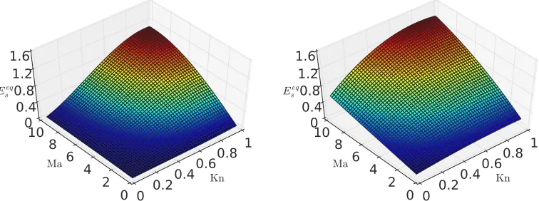
[image:5.608.114.492.72.210.2] [image:5.608.117.556.517.736.2]FIG. 9. (Color online) Dependence ofEeq
s on Kn and Ma in the bulk (left) and at the wall (right). We use the L2 norm to assess EcNSF and Eseq. In our
framework,Eseq assesses the nonequilibrium level andENSFc estimates the appropriateness of an NSF solution. As both these parameters are based purely on the molecular distribution function, we term them “kinetic breakdown parameters.”
In fact, both Eq. (6) and Eq. (7) are standard formulations for measurement of relative errors. Therefore,ENSF
c andE eq s are estimating the solution error relative to the correctionfNSF and the equilibrium functionfeq, respectively. It can be easily seen that a largerENSF
c means larger errors in the solution. Due to this direct connection, a “cutoff” value ofEcNSF, i.e., where a model switch should be conducted, may be determined from practical considerations. For example, a 10% error may be cho-sen as this value, as in the Couette flow cases discussed below.
III. NUMERICAL INVESTIGATION
To examine Eseq and EcNSF we first use shear-driven planar Couette flow as a benchmark. Here, the two bounding surfaces are moving with speedsUw in opposite directions, and their temperatures are set to T0. The Mach number is Ma=Uw/
√
RT0, and the Knudsen number is Kn=
√
π/2[μ0√RT0/(P0L)], whereL is the flow channel width andP0is the reference pressure. The NSF equations should be applicable for small Knudsen numbers, but will fail to predict the nonlinear Knudsen layers at the walls. Many proposed breakdown parameters are not appropriate for this type of flow, as already indicated from Fig.1. This therefore serves as a good benchmark case to evaluate different breakdown parameters.
We first investigate linear (low-speed) Couette flows. The simulations are accomplished by solving the linearized BGK equation with the discrete velocity method [36]. It is worth noting that all the quanities in this work are nondimension-alized using the system reported in Ref. [36] (see page 385). In Figs.2, 3, and 4 it is clearly seen thatEseq is negligibly small for low-speed Couette flows, even at relatively large Knudsen numbers (e.g., Kn=1). This indicates that the flows can be close to equilibrium at large Knudsen number, although the NSF equations will still fail. Therefore, alongside many other parameters, including the entropy generation rate and the parameter B,Eseq is not an appropriate breakdown parameter for the NSF equations or an NSF-order kinetic model. In Fig. 5, Eseq and EcNSF are explicitly plotted for two different Knudsen numbers: Eseq is smaller in the case
of larger Knudsen number (Kn=1), whileENSFc increases for increasing Knudsen numbers.
For nonlinear Couette flows (i.e., when Ma0.2), we perform molecular dynamics (MD) simulations using the OpenFOAM code that includes the MD routines implemented by Reese and coworkers [37–39]. Monatomic Lennard-Jones argon molecules are simulated [40], and initially the molecules are spatially distributed in the Couette flow domain with a random Gaussian velocity distribution corresponding to an initially prescribed gas temperature. They are then allowed to relax through collisions until reaching a steady state before we take measurements. This MD solver has been previously validated for both liquids and gases confined in arbitrary geometries. To achieve measurement of a smooth velocity distribution function at steady state, molecular velocity samples are taken in every time step (0.001τ, where τ = md2/, with m being the molecular mass, d the diameter of gas molecules, and being related to the interaction strength of the molecules) for a total time of at least 30 000τ (in the extreme rarefied and high speed flow case below, up to 100 000τ). We have 83 500 molecules in each simulation, and apply diffuse wall interactions.
The measurement sampling is performed in the micro-canonical ensemble consisting of a constant number of atoms, constant volume, and constant energy. Each case is solved in parallel on 16 cores of the 1100 core high performance com-pute facility at the University of Strathclyde. The equations of molecular motion are integrated using a leapfrog scheme with the simulation time step of 5 fs. The actual run time for each case ranges from 50 to 200 h, depending on the level of rarefaction, for which we were able to simulate 1000 ns of problem time after reaching the steady state. The simulation domain is divided into 80 bins in the wall-normal direction to measure macroscopic field properties, such as temperature. In each bin, there are approximately 1000 molecules in order to measure local macroscopic properties, and averaging occurs over 30–100 million time samples in the steady-state regime so as to minimize numerical errors.
The resulting profiles ofEseqandENSFc for various nonlinear Couette flow cases are presented in Figs.6,7, and8. In these flows nonequilibrium and rarefaction effects are coupled:Eseq shows the level of nonequilibrium in the local flowfield, while
ENSF
[image:6.608.115.493.74.215.2]FIG. 10. (Color online) Dependence ofENSF
c on Kn and Ma in the bulk (left) and at the wall (right).
FIG. 11. (Color online) Cross-channel profiles ofENSF
c predicted by a 16-velocity lattice model for linear Couette flows at Kn=0.1 and 1. The planar channel walls are at [−0.5,0.5].
FIG. 12. (Color online) Lid-driven cavity flow; profiles of errors of the velocity field along the horizontal lineY =0.627.
FIG. 13. (Color online) Lid-driven cavity flow; profiles ofENSF
[image:7.608.119.487.76.212.2] [image:7.608.115.492.242.376.2] [image:7.608.111.492.419.556.2] [image:7.608.112.494.587.728.2]FIG. 14. (Color online) Lid-driven cavity flow; profiles ofEeq
s predicted from the 400-velocity lattice model along the horizontal line Y =0.627.
Knudsen number. In contrast to the linear (low-Mach number) Couette flow case,Eseqseems to be able to indicate the error induced by the NSF model. This may be the reason why some parameters that measure deviation from equilibrium, such as Tsien’s parameter, the parameter B, and the entropy generation rate, have some success for high-speed flows. But onlyENSFc
works consistently, for both linear and nonlinear Couette flows, as a breakdown indicator for the NSF model or an NSF-order kinetic model.
To understand how the Knudsen and Mach numbers affect
EseqandEcNSF, we present their dependencies on Kn and Ma in Figs. 9 and 10. These clearly indicate the complicated coupled effects of rarefaction and nonequilibrium varying with the Knudsen number and the Mach number. When the Mach number is small, the flow is close to equilibrium regardless of the Knudsen number. For a smallEcNSF, the Knudsen number must be small; but EcNSF can also be significant when the Knudsen number is still small (see Fig.10). This indicates that an NSF solution may be invalid even with relatively small Knudsen numbers.
In the above cases, the parameters were evaluated using nu-merical solutions at molecular resolution. WhileEcNSFappears to be able to give reasonable indications, we wish to investigate now whether this parameter can use results from a less accurate model in order to assess whether it needs to switch to a more accurate model. In Ref. [19], we demonstrated how to couple two lattice Boltzmann models (e.g., with 16 and 36 lattice velocities for 2D simulations) at prescribed interfaces
where the lower-order model is employed on 70% of the com-putational region in the center of the channel. In Fig.11, the re-sults of the 16-velocity model are presented for linear Couette flows at Kn=0.1 and Kn=1. We see thatENSF
c calculated from this low-order model can reasonably indicate where the lower-order model needs to be switched to a higher-order model. For the case of Kn=0.1,ENSF
c predicts errors of about 10% aty = ±0.35, which indicates that it is better to switch models at these points. For the case of Kn=1,ENSF
c suggests that the higher-order model should be used exclusively, as the error is always larger than 60%. In both cases the predictions ofEcNSFare consistent with the practice in Ref. [19].
To further testENSF
c , we simulate a lid-driven cavity flow. In this flow, the gas is contained in a two-dimensional rectangular geometry with four walls. Both the length in thex direction and the height in the y direction are set to beL, which is therefore considered as the reference length to define the Knudsen number. The top wall is moving from left to right while the other three walls are stationary. The lid speed is set to be 0.01 and 0.0001 for various cases and is used to define the characteristic Mach number, i.e., the ratio of the lid speed and
√
RT0whereT0 is the wall temperature. The simulations are performed using lattice Boltzmann models for Kn=0.1 and Kn=1: NSF-level solutions are provided by the 9-velocity lattice Boltzmann model, while a 400-velocity model serves to provide the benchmark results. In these simulations, we compare with the error in the predicted velocity field, which is calculated as (uC−uE)2+(vC−vE)2/
√
u2C+v2C, where
[image:8.608.118.489.73.210.2] [image:8.608.115.494.592.732.2]may be attributed to the fact that the distribution functions contain more information than the macroscopic flow quantities used in LRS.
IV. CONCLUDING REMARKS
On the fundamental basis of the molecular velocity dis-tribution function, we have discussed how to evaluate the appropriateness of a locally applied continuum level kinetic solver for a gas flow. A breakdown parameter ENSF
c has
additional computational cost.
By using Couette flows and lid-driven cavity flows as test cases, we have demonstrated the encouraging capability of ENSF
c as a breakdown parameter. However, investigations of further flow problems are necessary in order to assess issues such as the cutoff value where a model switch should be conducted. Although EcNSF itself is mathematically a L2
norm form of error estimation, and so provides intuitive guidance, the determination of the cutoff value may be problem-dependent and needs to be calibrated by studying more flows.
[1] G. Karniadakis, A. Beskok, and N. Aluru, 1st ed.,Microflows and Nanoflows: Fundamentals and Simulation (Interdisci-plinary Applied Mathematics)(Springer, Berlin, 2005). [2] D. A. Lockerby, J. M. Reese, and H. Struchtrup,Proc. R. Soc.
A465,1581(2009).
[3] S. Tiwari, A. Klar, and S. Hardt,J. Comput. Phys.228,7109 (2009).
[4] Q. Sun, I. D. Boyd, and G. V. Candler,J. Comput. Phys.194, 256(2004).
[5] T. E. Schwartzentruber and I. D. Boyd,J. Comput. Phys.215, 402(2006).
[6] T. E. Schwartzentruber, L. C. Scalabrin, and I. D. Boyd, J. Comput. Phys.225,1159(2007).
[7] H. S. Wijesinghe and N. G. Hadjiconstantinou, Int. J. Mult. Comput. Eng.2,189(2004).
[8] P. L. Tallec and F. Mallinger,J. Comput. Phys.136,51(1997). [9] J.-F. Bourgat, P. L. Tallec, and M. D. Tidriri,J. Comput. Phys.
127,227(1996).
[10] S. T. O’Connell and P. A. Thompson,Phys. Rev. E52,R5792 (1995).
[11] J. M. Burt and I. D. Boyd,J. Comput. Phys.228,460(2009). [12] N. G. Hadjiconstantinou, Bull. Pol. Ac.: Tech53, 335 (2005). [13] I. D. Boyd, G. Chen, and G. V. Candler,Phys. Fluids7,210
(1995).
[14] W.-L. Wang and I. D. Boyd,Phys. Fluids15,91(2003). [15] D. A. Kessler, E. S. Oran, and C. R. Kaplan,J. Fluid Mech.661,
262(2010).
[16] G. A. Bird,Annu. Rev. Fluid Mech.10,11(1978). [17] S. M. Yen,Annu. Rev. Fluid Mech.16,67(1984).
[18] K. Xu and J.-C. Huang,J. Comput. Phys.229,7747(2010). [19] J. Meng, Y. Zhang, and X. Shan, Phys. Rev. E83, 046701
(2011).
[20] V. V. Aristov, A. A. Frolova, S. A. Zabelok, V. I. Kolobov, and R. R. Arslanbekov,Computational Fluid Dynamics 2006 (Springer, Berlin, 2009), pp. 719–724.
[21] V. I. Kolobov, R. R. Arslanbekov, V. V. Aristov, A. A. Frolova, and S. A. Zabelok,J. Comput. Phys.223,589(2007).
[22] K. Xu and Z. Li,J. Fluid Mech.513,87(2004). [23] H. S. Tsien, J. Aerospace Sci.13, 342 (1946). [24] G. A. Bird,AIAA J.8,1998(1970).
[25] S. Tiwari,J. Comput. Phys.144,710(1998).
[26] A. L. Garcia and B. J. Alder,J. Comput. Phys.140,66(1998). [27] M. N. Macrossan, in Twenty-Fifth International Symposium
on Rarefied Gas Dynamics, St. Petersburg, Russia, edited by M. S. Ivanov and A. K. Rebrov (Siberian Branch of the Russian Academy of Sciences, Russia, 2007), pp. 759–764.
[28] S. Chigullapalli, A. Venkattraman, M. S. Ivanov, and A. A. Alexeenko,J. Comput. Phys.229,2139(2010).
[29] S. Chapman and T. G. Cowling, 3rd ed., The Mathematical Theory of Non-Uniform Gases(Cambridge University Press, Cambridge, 1953).
[30] H. Struchtrup,Macroscopic Transport Equations for Rarefied Gas Flows: Approximation Methods in Kinetic Theory (Interac-tion of Mechanics and Mathematics)(Springer, Berlin, 2005). [31] H. Grad,Commun. Pure Appl. Maths2,331(1949).
[32] H. Struchtrup and M. Torrilhon,Phys. Fluids15,2668(2003). [33] X.-J. Gu and D. R. Emerson,J. Fluid Mech.636,177(2009). [34] G. A. Radtke, Jean-Philippe, M. Praud, and N. G.
Hadjiconstantinou, Philos. Trans. R. Soc. A371, 1471 (2013). [35] Y. Zheng and H. Struchtrup,Continuum Mech. Thermodynam.
16,97(2004).
[36] J. Meng, L. Wu, J. M. Reese, and Y. H. Zhang,J. Comput. Phys. 251,383(2013).
[37] G. B. Macpherson, M. K. Borg, and J. M. Reese,Mol. Simul. 33,1199(2007).
[38] G. B. Macpherson, and J. M. Reese,Mol. Simul.34,97(2008). [39] M. K. Borg, G. B. Macpherson, and J. M. Reese,Mol. Simul.
36,745(2010).


![FIG. 5. (Color online) Cross-channel comparison of EMach numbers. The planar channel walls are at [eqs (left) and ENSFc(right) for linear Couette flows at Kn = 0.01 and Kn = 1 for small−0.5,0.5].](https://thumb-us.123doks.com/thumbv2/123dok_us/1643947.117881/4.608.116.492.593.733/color-channel-comparison-numbers-channel-ensfc-linear-couette.webp)