City, University of London Institutional Repository
Citation
:
Borsato, R., Olsson-Sax, O., Sfondrini, A. and Stefanski, B. (2014). The complete AdS3 ×S3 × T4 worldsheet S matrix. Journal of High Energy Physics, 2014(10), doi: 10.1007/JHEP10(2014)066This is the published version of the paper.
This version of the publication may differ from the final published
version.
Permanent repository link: http://openaccess.city.ac.uk/4787/
Link to published version
:
http://dx.doi.org/10.1007/JHEP10(2014)066Copyright and reuse:
City Research Online aims to make research
outputs of City, University of London available to a wider audience.
Copyright and Moral Rights remain with the author(s) and/or copyright
holders. URLs from City Research Online may be freely distributed and
linked to.
JHEP10(2014)066
Published for SISSA by SpringerReceived: June 25, 2014
Revised: August 25, 2014
Accepted: September 15, 2014
Published: October 10, 2014
The complete AdS
3×
S
3×
T
4worldsheet S matrix
Riccardo Borsato,a Olof Ohlsson Sax,b Alessandro Sfondrinic and Bogdan Stefa´nski jr.d
aInstitute for Theoretical Physics and Spinoza Institute, Utrecht University,
Leuvenlaan 4, 3584 CE Utrecht, The Netherlands
bThe Blackett Laboratory, Imperial College,
London, SW7 2AZ, U.K.
cInstitut f¨ur Mathematik und Institut f¨ur Physik, Humboldt-Universit¨at zu Berlin, IRIS Geb¨aude,
Zum Grossen Windkanal 6, 12489 Berlin, Germany
dCentre for Mathematical Science, City University London,
Northampton Square, EC1V 0HB, London, U.K.
E-mail: [email protected],[email protected],
Abstract: We derive the non-perturbative worldsheet S matrix for fundamental excita-tions of Type IIB superstring theory on AdS3×S3×T4 with Ramond-Ramond flux. To this end, we study the off-shell symmetry algebra of the theory and its representations. We use these to determine the S matrix up to scalar factors and we derive the crossing equa-tions that these scalar factors satisfy. Our treatment automatically includes fundamental massless excitations, removing a long-standing obstacle in using integrability to study the AdS3/CFT2 correspondence. The present paper contains a detailed derivation of results first announced in arXiv:1403.4543.
Keywords: AdS-CFT Correspondence, Exact S-Matrix, Integrable Field Theories
JHEP10(2014)066
Contents1 Introduction 2
2 The off-shell symmetry algebra of superstrings on AdS3×S3 ×T4 4 2.1 Killing spinors for type IIB supergravity on AdS3×S3×T4 5 2.2 Type IIB superstring action on AdS3×S3×T4 6 2.2.1 A suitable vielbein and bosonic equations of motion 6 2.2.2 Green-Schwarz action before kappa gauge fixing 7 2.2.3 Neutral fermions and the kappa gauge-fixed action 9 2.2.4 First-order action and uniform light-cone gauge 10 2.2.5 Gauge-fixed action withso(4)1⊕so(4)2 bispinor fermions 13
2.3 Supercurrents 15
2.4 The Aalgebra 16
2.4.1 The massless sub-sector 18
2.4.2 Fermionic Poisson brackets 20
2.4.3 Computing the central chargeC in the full theory 21
3 Symmetry algebra 22
3.1 Fromsu(1|1)2
c.e. topsu(1|1)4c.e. 23
3.2 Representations in the near-plane-wave limit 24
3.2.1 Left representation 25
3.2.2 Right representation 26
3.2.3 Massless representation 26
4 Exact representations 27
4.1 Short representations of su(1|1)2c.e. 28
4.2 psu(1|1)4
c.e. representations for massive excitations 28
4.2.1 Bi-fundamental structure 29
4.2.2 Left-right symmetry 29
4.3 psu(1|1)4
c.e. representations for massless excitations 30
4.3.1 Bi-fundamental structure 30
4.3.2 Equivalent descriptions 30
4.3.3 Left-right symmetry 31
4.4 Representation coefficients 32
4.5 Corrections to the massless dispersion relation 33
5 S matrix 34
5.1 The su(1|1)2
c.e. invariant S matrices 36
5.2 The S matrix from a tensor product 37
5.2.1 Massive sector (••) 38
JHEP10(2014)066
5.2.3 Massless sector (◦◦) 39
5.2.4 Normalisation of the sectors 39
5.3 Physical and braiding unitarity 40
5.4 The Yang-Baxter equation 40
5.5 Crossing invariance 41
6 Discussion and outlook 43
A Index conventions 45
B Spinor and gamma matrix conventions 45
C Killing spinors and a preferred choice of vielbeins 47
D Proof of the identity (2.24) 51
E Useful identities for so(4) gamma matrices 52
F Relations between ΓA and so(4)
1 ⊕so(4)2 gamma matrices 52
G LWZ in so(4)1 ⊕so(4)2 components 54
H Equations of motion 55
I Poisson bracket for ηI and χI 56
J Some Poisson brackets used in section 2.4.1 57
K Derivation of equation (2.89) 59
L Oscillator algebra 60
M Parametrisation of su(1|1)2c.e. S-matrix elements 63
N Explicit form of the S-matrix elements 64
N.1 The mixed-mass sector 64
N.2 The massless sector 66
O Normalization of S-matrix elements 66
JHEP10(2014)066
1 IntroductionThe AdS/CFT correspondence is a remarkable equivalence between quantum gauge and gravity theories. In its simplest form it posits a strong/weak duality between superstring theories on AdSd+1 × M9−d, where M9−d is a (9−d)-dimensional compact space, and
d-dimensional Conformal Field Theories (CFTs) on the boundary of AdSd+1 [1–3]. This conjecture has inspired important advances in our understanding of quantum gravity and Quantum Field Theory (QFT). An intriguing feature of the AdS/CFT duality is the emer-gence of integrable structures in the ’t Hooft, or planar, limit [4] of certain classes of dual theories. The prototypical example is the case of type IIB strings on AdS5×S5 and the dual N = 4 Supersymmetric Yang-Mills (SYM) theory, see [5, 6] for a review. Following the discovery of the ABJM Chern-Simons theory [7], integrability was found also to un-derpin the duality between this CFT and Type IIA string theory on AdS4 ×CP3 in the planar limit.1 The key role of integrability in providing a quantitative handle on both the AdS5/CFT4 and AdS4/CFT3 dualities is rather striking. It hints very strongly that, for certain classes of dual pairs, integrability provides the right set of tools with which to investigate the AdS/CFT correspondence. As a result, identifying other dual pairs where integrable methods may be applicable is an important challenge in developing a detailed understanding of the AdS/CFT correspondence.
Another set of classes where integrability emerges are strings on AdS3 × M7 back-grounds with 16 real supersymmetries. The AdS3/CFT2 correspondence is a particularly important example of gauge/string duality. Historically, gravity on AdS3 gave rise to an early example of holography [9]. The gravity theory was found to have an (infinite-dimensional) conformal symmetry on the boundary whose central charge could be calcu-lated. Further, black hole solutions could be constructed in the gravitational theory [10,11] and their entropy was understood using holography [12]. Moreover, the D1-D5 brane sys-tem, whose near-horizon limit gives rise to the AdS3/CFT2 correspondence, has played a central role in the string theory derivation of the black-hole entropy formula [13]. At low energy, such a brane construction gives rise to a 1 + 1 dimensional supersymmetric Yang-Mills theory with matter multiples in the fundamental and adjoint representations, adding new features with respect toN = 4 SYM and ABJM theories.
In the context of string theory, it is natural to first consider AdS3 backgrounds with maximal supersymmetry. Such backgrounds have 16 real supersymmetries and come in two distinct types. String theory on AdS3 ×S3 ×T4 gives rise to the small N = (4,4) superconformal algebra [1,14],2while string theory on AdS3×S3×S3×S1 leads to the large
N = (4,4) superconformal algebra [15]. Both types of backgrounds can be supported by a mixture of Ramond-Ramond (R-R) and Neveu-Schwarz-Neveu-Schwarz (NS-NS) fluxes. In the case of pure NS-NS flux, much progress was made by studying the worldsheet theory with two-dimensional CFT techniques [16–22]. These results can be mapped onto the
1See [8] for a review and a more complete list of references. 2String theory on AdS
JHEP10(2014)066
D1-D5 system via S duality,3 which however acts in a non-perturbative and non-planarway. It is then natural to ask if backgrounds involving R-R fluxes can be studied more directly [23]. In particular, developing a quantitative understanding of the pure R-R string theory is essential in understanding generic unprotected properties of the D1-D5 system, and a starting point to tackling more general AdS3/CFT2 dualities.
With this motivation in mind, it was realised that the equations of motion of type II string theory on the pure R-R background are integrable [24]4 and that this extends to mixed fluxes as well [26]. This prompted an extensive investigation of the quantum integrability properties of these backgrounds [24, 25, 27–48], mainly by means of the S-matrix approach that proved successful in the case of AdS5/CFT4, see also [49] for a review. A new feature of the AdS3 backgrounds is the presence of massless fundamental excitations on the worldsheet. Because massless modes are notoriously difficult to in-corporate into integrability constructions [50–52], this presented an early challenge to fully understanding the AdS3/CFT2 correspondence using integrable methods. On the other hand, massive S-matrices and Bethe ansatz equations of AdS3 ×S3 ×T4 [34, 35] and AdS3×S3×S3×S1 [32,33] are relatively well-understood in the pure R-R case;5 the giant magnon associated to the massive modes was also understood some time ago [56,57]. In [31] massless modes were incorporated in the weakly-coupled spin-chain picture. On the string side, only very recently it has been shown how massless modes can be included in the classical integrability machinery [58]. Both of these results demonstrate that the real intricacies involved in understanding massless modes occur away from the weakly-coupled string and spin-chain regimes.
The aim of this paper is to present in detail how massless excitations can be included in the non-perturbative integrability picture, and how the non-perturbative asymptotic worldsheet S matrix for all fundamental particles can be found in the case of pure R-R AdS3×S3×T4 background. These results were first presented in [59].
Our analysis starts from the determination of the off-shell symmetry algebraA of the theory. Before light-cone gauge fixing, the symmetries of AdS3×S3 ×T4 are given by the AdS3×S3 superisometries6 psu(1,1|2)L⊕psu(1,1|2)R together with the T4 isometries.
Fixing light-cone gauge breaks some of these symmetries, and in particular halves the supersymmetries. We are interested in the symmetry generators that are linearly realised after gauge fixing, as the S matrix will have to commute with them. Such generators will sit in A, together with some additional central charges which are expected from the case of AdS5×S5[60–62]. We will determine the form of these and find, as it should be, that they have a non-trivial action only on states that do not satisfy the level-matching constraint (i.e.
3In fact, S duality acts on mixed-flux background by swapping R-R with NS-NS fluxes.
4Integrable structures were also recently found from studying the Gubser-Klebanov-Polyakov “spinning string” [25].
5The S matrix for mixed R-R and NS-NS fluxes has also been studied [42,43], but remains somewhat more puzzling, see [44]. Other integrable aspects of the mixed flux backgrounds have been investigated in [53–55].
6The two copies of
JHEP10(2014)066
off shell). Once the off-shell algebra of the theory is determined we will use it to constrainthe non-perturbative 2→2 S matrix, which will then satisfy the Yang-Baxter equation. Unlike what happened in AdS5/CFT4 [60–62], we cannot use the coset action [24,63– 65] for our calculations. The coset action requires the use of a particular kappa gauge [24], which does not allow for a straightforward quantization of the massless modes; see [28] for a discussion of the coset kappa gauge. We will therefore work with the Green-Schwarz ac-tion [66], in light-cone gauge. Furthermore, we take the decompactificaac-tion limit, whereby the world-sheet cylinder becomes a plane and the asymptotic states can be defined. It is interesting to note that our results give an example of integrability where the fermionic degrees of freedom do not enter the dynamics through a coset action; similar observa-tions have recently been made in integrable AdS backgrounds which preserve even less supersymmetry [67].
In this way, we are able to establish the off-shell symmetry algebra, including the non-linear momentum-dependent central extension reminiscent of [61]. As expected, the light-cone-gauge worldsheet theory is non-relativistic. Massive and massless excitations will then have periodic dispersion relations, with the energy of the latter being linear in the momentum for small values of it. Using these results, the two-body S matrix will follow immediately by symmetry arguments, and is fixed up to some dressing factors, for which crossing equations can be written down. As expected, the massive-sector S matrix of [34], including the crossing-invariant dressing factors of [35] can be consistently embedded in the full S matrix of the present paper.
This paper is structured as follows. In section 2 we consider the type IIB superstring action for AdS3×S3×T4 in light-cone gauge, and derive its conserved supercurrents. This is done at leading order in the fermions and at subleading order in the bosons. In section3 we study the symmetry algebra A and the representations that emerge from the super-current analysis. We find three short irreducible representations of the centrally extended
psu(1|1)4⊕so(4) algebra:7 two massive representations of dimension four, and one massless one of dimension eight. In section4we deform the representations found perturbatively in order to reproduce the correct non-linear central extension and shortening condition. We also comment on the possibility of quantum corrections to the massless dispersion relation, arguing that they would break part ofA. Using those exact representations, in section5we construct an invariant S matrix for all of the superstring’s excitations, including the mass-less ones, up to some dressing factors which we constrain by crossing symmetry. We con-clude in section6. We relegate the more technical aspects of our results to the appendices.
2 The off-shell symmetry algebra of superstrings on AdS3×S3 ×T4
In this section we compute the algebra A of off-shell symmetries for classical Type IIB superstring theory on AdS3×S3×T4. At first sight it may appear that the natural setting for this would be the coset action [24,63–65], since one can use the algebraic structure of
JHEP10(2014)066
the coset to facilitate the computations. The coset action is obtained from a Green-Schwarzaction [66] by fully fixing the kappa symmetry to the so-called coset gauge. While it is use-ful in the study of the classical integrability of this theory, the coset gauge leads to a kinetic term for the massless fermions which contains no quadratic piece. As a result, computing
A using Poisson brackets is not straightforward in the coset gauge. Instead, we will per-form the calculations using the Green-Schwarz action in the BMN light-cone kappa gauge. Explicit expressions up to quartic order in fermions have been recently found [68], but we will only work up to quadratic order in fermions and so will use the component action [69]. This section is divided into four parts. In section 2.1we find the Killing spinors of the background in the metric (2.1). In section2.2we write down explicitly the action for Type IIB superstrings on AdS3×S3×T4, both before and after imposing the kappa gauge along the BMN light-cone coordinates. In section 2.3 we write down the super-currents for the
Acharges and in section2.4 we compute the off-shell algebraAof the classical theory. In appendix A we establish our conventions.
2.1 Killing spinors for type IIB supergravity on AdS3×S3 ×T4
In this sub-section we construct the Killing spinors for type IIB supergravity on AdS3× S3×T4. Expressions for these are well-known in the literature [70,71]. We adapt these well-known calculations to the metric
ds2=ds2AdS3+ds2S3+dXidXi, (2.1)
where
ds2S3 = +
1−y32+y42 4 1 +y32+y42
4 !2
dφ2+ 1
1 +y23+y24 4
!2
(dy32+dy42) (2.2)
and
ds2AdS3 =−
1 +z21+z22 4 1− z21+z22
4 !2
dt2+ 1
1−z21+z22 4
!2
(dz12+dz22), (2.3)
since this metric is well suited for expansion around the BMN ground state.
The ten-dimensional Killing spinor equations of Type IIB supergravity on AdS3×S3× T4 with R-R flux are
Dmε1+ 1
24F //Emε
1 = 0, D
mε2− 1
24F //Emε
2= 0, (2.4)
where the covariant derivative is given by
DmεI =
∂m+1 4ω/m
εI, (2.5)
and the R-R field strength by
/
F = ΓABCFABC = 6(Γ012+ Γ345). (2.6)
As is shown in more detail in appendix C, these equations are solved by
JHEP10(2014)066
whereεI0 are constant 9+1 dimensional Majorana-Weyl spinors,8 which further satisfy1 2(1 + Γ
012345)εI = 1 2(1 + Γ
012345)εI
0 = 0. (2.8)
The matrices ˆM and ˇM depend on the AdS3 ×S3 coordinates and for later convenience we seperate out the dependence ontand φfrom the other coordinates by writing
ˆ
M =M0Mt, Mˇ =M0−1Mt−1, (2.9)
where
M0 =
1 q
1−z21+z22 4
1 +y32+y24 4
1−1 2ziΓ
iΓ012
1−1 2yiΓ
iΓ345
,
M0−1 = q 1
1−z21+z22 4
1 +y32+y24 4
1 +1 2ziΓ
iΓ012
1 +1 2yiΓ
iΓ345
,
(2.10)
and
Mt=e−
1
2(tΓ12+φΓ34), M−1
t =e+
1
2(tΓ12+φΓ34). (2.11)
2.2 Type IIB superstring action on AdS3×S3×T4
In this sub-section we write down the action for Type IIB superstring action on AdS3×S3× T4. In section2.2.1we begin by introducing a set of bosonic vielbeins, particularly adapted to the analysis in the remainder of this section, and expressing the bosonic equations of motion in terms of these. In section 2.2.2we write down the action to quadratic order in fermions. By picking suitably defined fermionic fields, our action realises the 16 unbroken supersymmetries of the background via linear shifts of the massive fermionic fields. In section 2.2.3 we write down the BMN light-cone kappa gauge-fixed action to quadratic order in fermions. Just as was done in [72], we find it useful to redefine the fermions further so that they are neutral under the u(1) charges associated with tand φ translations. The action is then re-expressed in first-order formalism and fully gauge-fixed in the uniform light-cone gauge in section2.2.4.
2.2.1 A suitable vielbein and bosonic equations of motion
The Lagrangian for the bosonic sigma model is given by
LB =− 1 2γ
αβE
αAEβBηAB, (2.12)
where EαA = EmA∂αXm denotes the pullback of the vielbein. LB is invariant under SO(1,9) rotations in tangent space. As a result, all vielbeins that describe the same metric will lead to the same bosonic equations of motion, up to field redefinitions. Nevertheless, picking a suitable vielbein may reduce substantially the computational complexity of the analysis. Since we will be working with the metric (2.1), one seemingly natural choice is to
JHEP10(2014)066
pick diagonal vielbeinsEmAgiven in equations (C.1) and (C.13). It turns out that, for thepurpose of understanding the realisation of supersymmetry in the Green-Schwarz action, it is instead more conventient to use vielbeins ˆKmA and ˇKmA, which are related to the EmA by orthogonal transformations
ˆ
KmA= ˆMABEmB, KˇmA= ˆMABEmB. (2.13)
The matrices ˆM and ˇM are defined in equations (C.26), (C.17) and (C.5). They follow from considering bilinears formed out of the Killing spinorsεI, (cf. equation (C.25)). As a result, as shown in equations (C.11) and (C.20), ˆKmA and ˇKmA satisfy the Killing vector equation (C.10) and generate the so(2,2)⊕so(4) =sl(2)⊕sl(2)⊕su(2)⊕su(2) isometry algebra of AdS3×S3.
The bosonic equations of motion that follow from LB are
0 =ηAB
∂α(γαβEmAEnB∂βXn)− 1 2γ
αβ∂
m(EnAEkB)∂αXn∂βXk
=γαβ
−1
2 ωkABEn A+ω
nABEkA
EmB+ηABEmA∂nEkB
∂αXn∂βXk
+ηABEmAEnB∂α(γαβ∂βXn),
(2.14)
where in the second line we have used the fact that EmA is covariantly constant. For a generic vielbein the first term above is nonvanishing. However, the vielbeins ˆKmAand ˇKmA satisfy the Killing vector equation which makes it vanish, see (C.9). Hence the equations of motion written in terms of the worldsheet pullbacks ˆKαA and ˇKαA are simply
∂α(γαβKˆβA) = 0, ∂α(γαβKˇβA) = 0. (2.15)
This form of the equations of motion is not only particularly simple, but will prove to be very useful in analysing the supersymmetries of string theory on this background.
2.2.2 Green-Schwarz action before kappa gauge fixing
In this sub-section we write down the Green-Schwarz action for a superstring propagating in AdS3×S3×T4 up to quadratic order in fermions and construct supercharges preserving the non-gauge-fixed action. The Green-Schwarz action for Type IIB superstrings in a generic supergravity background was constructed in terms of superfields in [66], and explicit expres-sions in terms of fields are known to quadratic [69] and quartic order [68] in the fermions. We will perform a field redefinition of the conventional fermions [69] so that the 16 real supersymmetries of this background are realised as linear shifts of the massive fermions.9
The Green-Schwarz Lagrangian can be written as
L=LB+Lkin+LWZ. (2.16)
JHEP10(2014)066
The bosonic Lagrangian LB was discussed in the previous sub-section. We have split thefermionic Lagrangian into two terms: a term dependent on the worldsheet metric,Lkin, and the Wess-Zumino termLWZ. In the background we are considering, the former term is [69]
Lkin =−iγαβθ¯IE/α
δIJDβ+ 1 24σ
IJ
3 F //Eβ
θJ, (2.17)
where ¯θI = θ†IΓ0 and we have redefined the fermions compared to Cvetiˇc, L¨u, Pope and Stelle [69]
θ1 CLPS =
θ1+θ2
√
2 , θ2 CLPS=
θ1−θ2
√
2 , (2.18)
so that they enter diagonally in Lkin.
Next we define new fermions ϑ±I which are related to θI by
θ1 = 1 2(1 + Γ
012345) ˆM ϑ+ 1 +
1 2(1−Γ
012345) ˆM ϑ− 1,
θ2 = 1 2(1 + Γ
012345) ˇM ϑ+ 2 +
1 2(1−Γ
012345) ˇM ϑ− 2,
(2.19)
where the matrices ˆM and ˇM were given in (2.9). Inserting this into the Lagrangian and using the relations in appendix Cwe find
Lkin=−iγαβ
¯
ϑ−I K/ˆα∂βϑ−I + 2 ¯ϑ+I E/¯¯α∂βϑ−I + ¯ϑ+I K/ˆα∂βϑ+I
−1
2σ 3
IJϑ¯+IΓ012ϑ+J( ˆKαaKˆβbηab+ ¯E¯αa˙E¯¯
˙
b βηa˙b˙)
.
(2.20)
The definitions of the vielbeins appearing above are given in equations (2.13) and (C.27). The LagrangianLB+Lkin is invariant under the supersymmetry transformations
δϑ−I =ǫI, δϑI+= 0, δKˆαA=−i¯ǫIΓA∂αϑI−, δE¯¯α = 0, (2.21)
where in the above equation the index A= 0, . . . ,5. By imposing the Majorana condition on the fermions this gives us the expected 16 real supersymmetries of the background.
We now consider the Wess-Zumino term10
LWZ= +iǫαβ
¯
θ2E/α
Dβ+ 1 24F //Eβ
θ1+ ¯θ1E/α
Dβ− 1 24F //Eβ
θ2
(2.22)
After introducing the rotated fermions we find
LWZ= +iǫαβ
¯
ϑ−2Mˇ−1M /ˆKˆα∂βϑ−1 + 2 ¯ϑ+2Mˇ−1M /ˆE¯¯α∂βϑ−1 + ¯ϑ+2Mˇ−1M /ˆKˆα∂βϑ+1
+ ¯ϑ−1Mˆ−1M /ˇKˇα∂βϑ−2 + 2 ¯ϑ+1Mˆ−1M /ˇE¯¯α∂βϑ−2 + ¯ϑ+1Mˆ−1M /ˇKˇα∂βϑ+2
− 1
2ϑ¯ +
2Mˇ−1Mˆ(K/ˆαK/ˆβ+E/¯¯αE/¯¯β)Γ012ϑ+1
+ 1 2ϑ¯
+
1Mˆ−1Mˇ(K/ˇαK/ˇβ+E/¯¯αE/¯¯β)Γ012ϑ+2
.
(2.23)
JHEP10(2014)066
This term is also invariant to quadratic order in the fermions under the supersymmetrytransformations (2.21). To see this we can use the identity
ǫαβ∂α Mˇ−1M /ˆKˆβ
(1−Γ012345) = 0 (2.24)
to show that
ǫαβϑ¯−2Mˇ−1M /ˆKˆα∂βϑ−1 =ǫαβϑ¯−1Mˆ−1M /ˇKˇα∂βϑ−2 , (2.25)
up to a total derivative. In appendixDwe prove (2.24). Together with an obvious extension of the above argument to expressions involving ˇK instead of ˆK, the Lagrangian LWZ can therefore be written in a form where ϑ−I only appears with a partial derivative acting on it, making the symmetry under shifts of that fermion manifest.
2.2.3 Neutral fermions and the kappa gauge-fixed action
In this sub-section we impose the BMN light-cone kappa gauge on the Lagrangian obtained in the previous sub-section. In addition, we will further redefine the fermions. Recall that the tangent space rotations (2.19) introduced in the previous section were useful for obtaining the supersymmetry transformations before fixing kappa gauge. However,
ˆ
KmA and ˇKmA, and therefore also the fermions ϑ±I, transform nontrivially under shifts of the coordinates tand φ. When imposing uniform light-cone gauge it is useful to work with fermions that are uncharged under these shifts [72], which motivates the further re-definition of the fermions.11
To perform this field redefinition, recall that the rotation matrices ˆM and ˇM can be written in terms of the matricesM0 and Mt (see equation (2.9)), whereM0 is independent oftandφwhileMtonly depends on those two coordinates. In order to have fermions that are uncharged under shifts of tand φone needs to multiply the fermions ϑ±1 byMt−1 and the fermionsϑ±2 withMt. In other words, we define
θ1 = 1 2(1 + Γ
012345)M
0χ1 + 1 2(1−Γ
012345)M 0η1
θ2 = 1 2(1 + Γ
012345)M−1 0 χ2+
1 2(1−Γ
012345)M−1 0 η2.
(2.26)
We also need to perform the corresponding rotation on the vielbeins defining new vielbeins ˆ
E and ˇE,
/ˆ
K =Mt−1EM/ˆ t, K/ˇ =MtEM/ˇ t−1. (2.27)
The components of the inverse vielbeins can easily be read off from equations (C.7) and (C.19) by dropping the first t- and φ-dependent factor.
It is useful to introduce light-cone coordinates
E±= 1 2(E
5±E0), x±= 1
2(φ±t). (2.28)
This leads to
Ex++ =Ex−− = 1 2 E
5
φ+Et0
, Ex−+ =Ex+− = 1 2 E
5
φ−Et0
. (2.29)
JHEP10(2014)066
The light-cone components of the tangent space metric are given byη+−=η−+= +1
2, η+−=η−+= +2. (2.30)
The bosonic Lagrangian then takes the form
LB =− 1 2γ
αβ 4E+
αEβ−+EαiEβi +EαiEβi
. (2.31)
We will work in the BMN light-cone kappa gauge
Γ+ηI = 0, Γ+χI = 0, Γ±= 1 2 Γ
5
±Γ0. (2.32)
The kappa gauge-fixed Lagrangian then takes the form
Lkin=−2iγαβ
¯
η1Eˆα+Γ−∂βη1−η¯1Γ012η1Eˆα+∂βx++ ¯η2Eˇα+Γ−∂βη2+ ¯η2Γ012η2Eˇα+∂βx+
+ ¯χ1Eˆα+Γ−∂βχ1− 1 4χ¯1Γ
012χ 1
X5
A,B=0 ˆ
EαAEˆβBηAB+ ¯E¯αiE¯¯βi −4 ˆEα+∂βx−
+ ¯χ2Eˇα+Γ−∂βχ2+ 1 4χ¯2Γ
012χ 2
X5
A,B=0 ˇ
EαAEˇβBηAB+ ¯E¯αiE¯¯βi −4 ˇEα+∂βx−
.
(2.33)
LWZ= +iǫαβ
¯
η2E/ˇαM02∂βη1+ ¯η2E/ˇαM02Γ12η1∂βx+
+¯η1E/ˆαM0−2∂βη2−η¯1E/ˆαM0−2Γ12η2∂βx+
+ ¯χ2E/ˇαM02∂βχ1−χ¯2E/ˇαM02Γ12χ1∂βx−− 1
2χ¯2(E/ˇαE/ˇβ+ / ¯ ¯
EαE/¯¯β)M02Γ012χ1
+ ¯χ1E/ˆαM0−2∂βχ2+ ¯χ1E/ˆαM0−2Γ12χ2∂βx−+ 1
2χ¯1(E/ˆαE/ˆβ+ / ¯ ¯
EαE/¯¯β)M0−2Γ012χ2
+2 ¯χ2E/¯¯αM02∂βη1+ 2 ¯χ2E/¯¯αM02Γ12η1∂βx+
+2 ¯χ1E/¯¯αM0−2∂βη2−2 ¯χ1E/¯¯αM0−2Γ12η2∂βx+
. (2.34)
2.2.4 First-order action and uniform light-cone gauge
To fix the bosonic gauge we will impose uniform light-cone gauge [74]. The simplest way to introduce this gauge is to rewrite the action in a first-order formalism by introducing coordinates xM
pM =
δS
δx˙M. (2.35)
From the definition of the light-cone coordinates x± we then have
JHEP10(2014)066
The isometries generated by shifts intandφlead to the conservation of the energyE andangular momentumJ
E =−
Z +r
−r
dσ pt, J = + Z +r
−r
dσ pφ, (2.37)
where−r≤σ < r denotes the range ofσ. For the light-cone momenta we then find
P+ = Z +r
−r
dσ p+=J−E, P−= Z +r
−r
dσ p− =J+E. (2.38)
The uniform light-cone gauge fixing is now obtained by setting12
x+=τ, p−= 2. (2.39)
To make the origin of various expressions more clear we generally still write out factors of
p−, unless this clutters our formulae excessively. In any case, the correct factors ofp−can be restored from dimensional considerations.
To see how this gauge works let us consider the bosonic first-order action, which takes the form
SB= Z +r
−r
dσ dτ
p+x˙++p−x˙−+pix˙i+pix˙i+
γ01 γ00C1+
1 2γ00C2
, (2.40)
where
C1 =p+x′++p−x′−+pix′i+pix′i (2.41)
and
C2=G++p+p++ 2G+−p+p−+G−−p−p−+Gijpipj +Gijpipj
+G++x′+x′++ 2G+−x′+x′−+G−−x′−x′−+Gijx′ix′j+Gijx′ix′j.
(2.42)
The equations of motion for the worldsheet metric leads to the Virasoro constraintsC1= 0 and C2= 0. Sincex′+= 0 we can solve the first constraint by
′
x− =− 1
p−
pix′i+pix′i
. (2.43)
Inserting this into the expression for C2 we can solve the second constraint for p+. The gauge-fixed action can then be written as13
SB = Z +r
−r
dσ pix˙i+pix˙i−HB
, (2.44)
with
HB=−p+. (2.45)
12The integrals in (2.37) and (2.38) that yields our charges are normalised as in (2.4) of [5], but our definition of the light-cone momentum p− is different and later we imposep− = 2 rather than p− = 1. Here we only consider string states with zero winding number. For more general states the gauge fixing condition becomesx+=τ+1
2 π
rmσ, wheremis the integer winding number along the angleφ. 13We have omitted the total derivative termp
JHEP10(2014)066
For the transverse fields we impose periodic boundary conditions14 xi(+r) = xi(−r) andxi(+r) = xi(−r). Since we further assume there is no winding along the angle φ, we find that a physical state should satisfy the level matching condition
∆x−=x−(+r)−x−(−r) = Z +r
−r
dσ ′
x−= 0. (2.46)
The gauge-fixed action is invariant under worldsheet translations, which leads to the con-servation of the worldsheet momentum
pws =− Z +r
−r
dσ pix′i+pix′i =p−∆x−. (2.47)
From the level matching constraint we then find that a physical string in the zero winding sector has to have vanishing total worldsheet momentum
pws= 0. (2.48)
In order to study the worldsheet S matrix we need to be able to create well-defined asymptotic states to scatter. To do this we will from now on work in the decompactification limit by sending the parameterr, which gives the circumference of the worldsheet cylinder, to infinity. Note that after gauge fixing, the light-cone momentumP− is given by
P−= Z +r
−r
dσ p− = 4r. (2.49)
Hence, in the large-r limit the light-cone momentum becomes infinite.
By imposing periodic boundary conditions on the T4 coordinates xi we are ignoring winding modes on the torus. This is justified since we study local properties of the field theory on the worldsheet and work in the decompactification limit. If we begin with a string state in the zero winding sector and act on the state with a symmetry generator that acts locally, there is no way to obtain a state with non-zero winding. Similarly, the scattering of two excitations without any winding will not result in non-trivial winding of the out-going states. In the zero-winding sector the u(1)4 shift isometries of the T4 are supplemented by anso(4) symmetry, which we will discuss in the next subsection and will play an important role inA when we will use it to constrain the S matrix.
It is furthermore possible to check that, as long as we are in the decompactified theory with P− = ∞, the light-cone Hamiltonian takes the same form in any sector with finite winding on T4. This indicates that the S matrix that we will find by this treatment should be valid in any winding sector, and should not depend on the moduli of T4. The depen-dence of the spectrum on winding numbers and torus moduli should then manifest itself only at the level of the Bethe-Yang equations, as it happens in the case of orbifolds, see e.g. [75,76] for a review.
JHEP10(2014)066
2.2.5 Gauge-fixed action with so(4)1⊕so(4)2 bispinor fermionsThe fermions appearing in the action (2.33), (2.34) are 32-component 9+1-dimensional spinors. However, these spinors satisfy a number of projections: the 9+1-dimensional Weyl projection, the kappa gauge condition (2.32) as well as equation (2.26). Because of these, writing the fermions as 32 component spinors is rather redundant. In this sub-section we will write down the fully gauge-fixed action in terms of non-redundant physical spinors. As a result of the above projections, the physical spinorsηI andχI are in fact bispinors of so(4)1 ⊕so(4)2 ⊂ so(8), with so(8) corresponding to rotations transverse to light-cone directions. The algebrasso(4)1 andso(4)2correspond to rotations along the non-light-cone AdS3 ×S3 and T4, directions, respectively.15 While the latter algebra remains unbroken by the background, so(4)1 is in fact broken to so(2)⊕so(2), as can be already seen in the plane-wave limit [77,78]. We will see this breaking in the Lagrangian we write down in this subsection. Nevertheless, it is still convenient to express the fermionic fields that enter the Lagrangian as bispinors ofso(4)1⊕so(4)2. We will use the indicesa, ˙a(respectively,a, ˙a) to denote the positive and negative chiralityso(4)1 (so(4)2) spinors. Further, we introduce gamma matrices, ˆγi withi= 1,2,3,4 and ˆτi,i= 6,7,8,9 forso(4)
1 andso(4)2 . We write these matrices as16
(ˆγi)aa˙bb˙ =
0 (γi)ab˙ (˜γi)a˙b 0
!
, (ˆτi)aa˙bb˙ = 0 (τ
i)a
˙
b (˜τi)a˙b 0
!
, (2.50)
with the Clebsch-Gordan coefficients for the decomposition of two so(4) Weyl spinors of opposite chirality given by
γ1 = +σ3, γ2 =−i1, γ3= +σ2, γ4 = +σ1, ˜γi = +(γi)†,
τ6 = +σ1, τ7 = +σ2, τ8= +σ3, τ9 = +i1, τ˜i =−(τi)†.
(2.51)
The notation introduced above is purposefully reminiscent of the light-cone gauge in flat space [79] but our exact conventions are slightly different to, for example, those in [80]. The matrices ˆγi and ˆτi satisfy the Clifford algebra relations
{γˆi,ˆγj}= +2δij, (ˆγi)t= +tˆγit−1,
{τˆi,τˆj}=−2δij, (ˆτi)t=−sτˆis−1, (2.52)
wheret=s=σ3⊗σ2. We also introduce
(γij)ab = 1 2(γ
iγ˜j −γj˜γi)a
b, (τij)ab= 1 2(τ
iτ˜j−τjτ˜i)a b,
(˜γij)a˙b˙ = 1 2(˜γ
iγj −γ˜jγi)a˙ ˙
b, (˜τij)a˙b˙= 1 2(˜τ
iτj−˜τjτi)a˙ ˙
b,
(2.53)
15In the next section we will write the T4 part of this algebra asso(4)
2=su(2)•⊕su(2)◦.
16The matricesγi
JHEP10(2014)066
so that the Lorentz generators take the formˆ
γij = γ ij 0
0 ˜γij
!
, τˆij = τ ij 0
0 ˜τij
!
. (2.54)
Some useful relations involving these gamma matrices are collected in appendixE. In order to obtain compact expressions for the gauge-fixed action we find it necessary to perform a change of basis on the gamma matrices presented in appendixB. These matrices are written as tensor products of five 2×2 matrices. Our change of basis takes the form
m1⊗m2⊗m3⊗m4⊗m5 →n1⊗n2⊗n3⊗n4⊗n5 (2.55)
with
n1 =m1, n2⊗n3 =P(m3⊗m4)P−1, n4⊗n5 =m2⊗m5, (2.56)
and
P =
0 1 0 0 0 0 1 0 0 0 0 1 1 0 0 0
. (2.57)
With this change of basis,so(4)1 and so(4)2 act non-trivially only on n2⊗n3 and n4⊗n5, respectively, while the 9+1-dimensional Weyl projection acts only onn1. The kappa gauge-fixed spinors satisfy
Γ1234χI = +χI, Γ6789χI = +χI, Γ1234ηI =−ηI, Γ6789ηI =−ηI. (2.58)
Since the action of Γ1234 and Γ6789 reduces to ˆγ1234 and ˆτ6789 when acting onη
I and χI we see thatχI and ηI carry indices
(χI)ab, (ηI)a˙b˙. (2.59)
Having introduced this notation we can now re-write Lkin in equation (2.33) as17
Lkin=−2iγαβ "
ˆ
Eα+η¯1∂βη1+ ˇEα+η¯2∂βη2+ ˆEα+χ¯1∂βχ1+ ˇEα+χ¯2∂βχ2
−∂αx+ Eˆβ+η¯1γ˜34η1+ ˇEβ+η¯2γ˜34η2
−1
4 X5
A,B=0 ˆ
EαAEˆβBηAB+ ¯E¯αiE¯¯βi −4 ˆEα+∂βx−
¯
χ1γ34χ1
+1 4
X5
A,B=0 ˇ
EαAEˇβBηAB+ ¯E¯αiE¯¯βi −4 ˇEα+∂βx−
¯
χ2γ34χ2 #
.
(2.60)
JHEP10(2014)066
Above, we have suppressed the spinor indices for compactness and defined¯
ηI ≡(ηI)b˙b˙ǫb˙a˙ǫb˙a˙, χ¯I ≡(χI)bbǫbaǫba. (2.61)
Re-writingLWZ in equation (2.34) in terms ofso(4)1 and so(4)2 bispinors one arrives at a longer expression which we have relegated to appendix G.
The above Lagrangian still depends on the worldsheet metric. As discussed above, one way to complete the light-cone gauge fixing is to go to first-order formalism and solve the Virasoro constraints. Alternatively we can impose the conditionp−= 2 by solving for the worldsheet metric. Doing this we find that to the relevant order the metric is diagonal with components
γ00=−1 +1 2(z
2−y2) +1 8(z
2+y2)( ˙z2+ ′
z2+ ˙y2+ ′
y2−(z−y)2),
γ11= +1 +1 2(z
2−y2) +1 8(z
2+y2)( ˙z2+ ′
z2+ ˙y2+ ′
y2+ (z−y)2).
(2.62)
The derivatives of the nondynamic fieldx−can then be found from the Virasoro constraints.
2.3 Supercurrents
In section 2.2.2 we wrote down an action which realised linearly all 16 supersymmetries of our background. However, half of the supervariations (2.21) are incompatible with the BMN light-cone kappa gauge choice (2.32). This is a well known aspect of the light-cone gauge formalism [81] — it implies that such supervariations have to be combined with a compensating kappa transformation in order to preserve the gauge choice (2.32). The eight supercharges that commute with the Hamiltonian and form the fermionic part of A are associated with variations of precisely of this form.
Since kappa gauge transformations are known explicitly [66], it is in principal possible to find expression for such compensating kappa gauge transformations. The procedure is however computationally involved. To simplify matters, we will write down the supercur-rents corresponding to the Asupercharges to first order in fermions and third order in the transverse bosons. When computing the algebra A later in this section we will only need these expressions.
For notational convenience, we split the full supercurrent into parts involving only massless fields, only massive fields and a part involving a mix of massive and massless fields,
jIα =jI,αmassless+jαI,massive+jI,αmixed, I = 1,2. (2.63)
The supercurrents are given by
j1τ,massless =e+x−γ34x˙iγ34τ˜iχ1−x′iγ34τ˜iχ2
,
j2τ,massless =e−x−γ34x˙iγ34τ˜iχ2−x′iγ34τ˜iχ1
,
JHEP10(2014)066
j1τ,mixed=e+x−γ34
−1
2(z
2−y2)( ˙xiγ34τ˜iχ
1+x′iγ34τ˜iχ2) +ziyjx′iγ34γijτ˜iχ2
+1 2x˙·
′
x(zi−yi)γ34γiη2+ 1 4( ˙x
2+ ′
x2)(zi−yi)γ34γiη1
,
j2τ,mixed=e−x−γ34
−1
2(z
2−y2)( ˙xiγ34τ˜iχ
2+x′iγ34τ˜iχ1) +ziyjx′iγ34γijτ˜iχ1
−1
2x˙· ′
x(zi−yi)γ34γiη1−1 4( ˙x
2+ ′
x2)(zi−yi)γ34γiη2
,
(2.65)
j1τ,massive =e+x−γ34( ˙zi−y˙i)γiη1+ (zi+yi)γ34γiη1−(z′i−y′i)γiη2
,
j2τ,massive =e−x−γ34( ˙zi−y˙i)γiη2−(zi+yi)γ34γiη2−(z′i−y′i)γiη1
.
(2.66)
j1σ,massless=−e+x−γ34′
xiγ34τ˜iχ1−x˙iγ34τ˜iχ2
,
j2σ,massless=−e−x−γ34′
xiγ34τ˜iχ2−x˙iγ34τ˜iχ1
,
(2.67)
j1σ,mixed=−e+x−γ34
+1
2(z
2−y2)(′
xiγ34τ˜iχ1−x˙iγ34τ˜iχ2) +ziyjx˙iγ34γijτ˜iχ2
+1 2x˙·
′
x(zi−yi)γ34γiη1+ 1 4( ˙x
2+ ′
x2)(zi−yi)γ34γiη2
,
j2σ,mixed=−e−x−γ34
+1
2(z
2−y2)(′
xiγ34τ˜iχ2−x˙iγ34τ˜iχ1) +ziyjx˙iγ34γijτ˜iχ1
−1
2x˙· ′
x(zi−yi)γ34γiη2− 1 4( ˙x
2+ ′
x2)(zi−yi)γ34γiη1
,
(2.68)
j1σ,massive =−e+x−γ34(′
zi− ′
yi)γiη1−( ˙zi−y˙i)γiη2−(zi+yi)γ34γiη2
,
j2σ,massive =−e−x−γ34(′
zi− ′
yi)γiη2−( ˙zi−y˙i)γiη1+ (zi+yi)γ34γiη1
.
(2.69)
Above, for the massive part of the supercurrents we have only written down the lowest-order-in-bosons expression since it will be all we need later on. For compactness we have also suppressed all spinor indices; re-instating these we have, for example,
γ34τ˜iχ1 ≡(γ34)ab(˜τi)a˙b(χ1)bb. (2.70)
Using the equations of motion, which are presented in appendix H, we have checked that the currents satisfy the equation
∂τjIτ +∂σjIσ = 0, (2.71)
and hence are conserved.
2.4 The A algebra
JHEP10(2014)066
sub-leading order in bosons. This is the same order to which the corresponding algebrawas computed for Type IIB strings on AdS5×S5 [61]. Before describing the details of the computations, let us pause briefly to make two general observations.
Firstly, on-shell A reduces to psu(1|1)4 extended by the Hamiltonian and a central angular momentum and by the torus isometries. This is simply the part of superisometries of the classical string theory on AdS3 ×S3×T4 that commutes with the Hamiltonian, and amounts to psu(1|1)4⊕u(1)2⊕so(4). The important consistency check then is to see that when going off-shell, by relaxing the level-matching condition, the algebra becomes centrally extended in just the right way. In other words, the Poisson bracket between two different supercharges should result in an expression of the form
{(Q1)aa˙,(Q2)bb˙}
PB=−i C
ab,a˙b˙, (2.72)
where the matrix on the right-hand side can be decomposed into the two central charges extending the symmetry algebra.
Secondly, we note that the massive (yi, zi and ηI) and the massless fields (xi and χI) each form a consistent closed sector of the equations of motion of the theory. In the classical theory the massive sector is isomorphic to a closed sub-sector of the Type IIB string on AdS5×S5.18 As a result, the off-shell computation ofAin the massive sub-sector is identical to the computation performed in [61] and so we will not repeat it here. Instead, we will perform two types of computations that are new to Type IIB strings on AdS3×S3×T4. In section 2.4.1 we restrict to the massless sector of the theory and compute the off-shell algebra A; as anticipated in the previous paragraph, we explicitly see that on-shell the algebra does indeed reduce to psu(1|1)4⊕u(1)2. In section 2.4.3, we compute, off-shell, in the full massive and massless theory the relation (2.72).
We only determine the part of the central charges that depend on the bosonic fields. Since the central charges have to vanish for zero total worldsheet momentum this is enough to reconstruct the full charges. As we will see, the momentum dependence of the central charges comes in through the nonlocal and nondynamic field x−. To capture this depen-dence we employ a “hybrid” expansion similar to what was used in AdS5×S5 in [61]. This means that we expand the action in the transverse fields to quadratic order in fermions and quartic order in the transverse bosons, but keep any explicit factors ofx−unexpanded. This allows us to capture the full momentum dependence of the central charges. It is worth noting at this point that central extensions of the on-shell algebra of this kind had been studied for the plane-wave limit of AdS3×S3×T4 in [77].
The fermions in the Lagrangian (2.60) and (G.6) do not have a canonical kinetic term and so will not have a conventional Poisson bracket. It is possible to further redefine the fermionic fields order by order in the field expansion to correct this. However, for our purpose it will be simpler to work with the non-canonical Poisson bracket for the fermions that follows from the Lagrangian (2.60) and (G.6). The Poisson bracket of the fermions ηI and χI is presented below.
JHEP10(2014)066
2.4.1 The massless sub-sectorAs we have noted above, the equations of motion of our system are such that it is consistent to set the transverse massive excitations to zero. In this sub-section we focus on computing
A in the purely massless sector. This sector turns out to have a number of simplifying features compared to the full theory and so serves as a good warm-up exercise. We will therefore repeat some of the steps discussed above in more detail. What is more, this sector is not described by a semi-symmetric space coset and so understanding how it enters the integrable machinery is one of the central results of this paper. The massless part of the gauge fixed Lagrangian is given by
L(Bm)=−1
2γ αβ4∂
αx+∂βx−+∂αxi∂βxi
L(kinm)=−2iγαβ
¯
χI∂αχI∂βx+− 1 4σ
3
IJχ¯Iγ34χJ∂αxi∂βxi
,
L(WZm)=−2iǫαβ
σIJ1 χ¯I∂αχJ∂βx++ǫIJ 1 4χ¯Iγ
34τijχ
J∂αxi∂βxj
.
(2.73)
The massless parts of the supercurrents were given in equations (2.64) and (2.67). Notice that to this order in fermions the supercurrents do not contain a term cubic in the bosons, and are in fact the same as they would be in flat space.19 The non-linear terms in the equations of motion for the fermions are exactly cancelled by the nonlocal exponential part of the supercurrents.
We now want to calculate the algebra Aobtained by taking Poisson brackets between the supercharges obtained from the currents. To do this we write the action in first-order formalism. The conjugate momenta of the bosonic fields are given by
p−=
δS
δx˙− =−2γ 0β∂
βx+,
p+=
δS
δx˙+ =−2γ 0β∂
βx−−2iγ0βχ¯I∂βχI + 2iσ1IJχ¯Iχ′J,
pi=
δS δx˙i =−γ
0β∂
βxi+iγ0βσIJ3 χ¯Iγ34χJ∂βxi−iǫIJχ¯Iγ34τijχJx′j.
(2.74)
Inserting this into the Lagrangian we get
L(m)=p−x˙−+pix˙i+ip−χ¯Iχ˙I +
γ01 γ00C1+
1
2γ00C2, (2.75)
with the constraints given by
C1 =p−x′−+pix′i+ip−χ¯Iχ′I,
C2 =p+p−+pipi+x′2−2ip−σIJ1 χ¯Iχ′J+iσ3IJχ¯Iγ34χJ(pipi−x′2)
+ 2iǫIJχ¯Iγ34τijχJpix′j.
(2.76)
JHEP10(2014)066
By solving the constraint C1= 0 we obtain′
x−=− 1
p−
pix′i−iχ¯Iχ′I. (2.77)
Up to quadratic order in the fermions the massless Hamiltonian density H(m) = −p + is given by
H(m)= 1
p−
pipi+x′2−2ip−σIJ1 χ¯Iχ′J
+iσIJ3 χ¯Iγ34χJ(pipi− ′
X2) + 2iǫIJχ¯Iγ34τijχJpix′j.
(2.78)
From the kinetic term of the action we can read off the (canonical) Poisson brackets
[xi(σ), pj(σ′)]
PB =δ
i
jδ(σ−σ′),
{(χI)aa(σ),(χJ)bb(σ′)}
PB =−
i
2p−
ǫabǫabδ(σ−σ′).
(2.79)
Using results from appendix J one can check that the supercharge densities
Q1 =e+γ 34x−
piτ˜iχ1−x′iτ˜iχ2≡e+γ 34x−
Q(2)1 , (2.80)
Q2 =e−γ 34x− ′
xiτ˜iχ1−piτ˜iχ2
≡e−γ34x−Q(2)2 (2.81)
both lead to conserved charges
QI = Z r
−r
dσQI, [Q1, H(m)]
PB = [Q2, H (m)]
PB= 0. (2.82)
Next we note that up to integrating by parts20
{(Q(2)1 )aa˙,(Q(2)1 )bb˙}
PB = +
i
2p−
ǫabǫa˙b˙pipi+x′2−2ip−σIJ1 χ¯Iχ′J
. (2.83)
The last term in the expression in the bracket is exactly the quadratic Hamiltonian in the massless sector. So up to quadratic order in excitations we find
{(Q1)aa˙,(Q1)bb˙} PB= +
i
2 Z +∞
−∞
dσ e+γ34x−ac e+γ
34x−b
dǫcdǫa˙
˙
bH(m)
= +i 2ǫ
abǫa˙b˙H(m).
(2.84)
Similarly we can calculate the commutator between two different supercharges
{(Q(2)1 )aa˙,(Q(2)2 )bb˙}
PB=
i p−
pix′i−χ¯Iχ′I
ǫabǫa˙b˙
=−i′
x−ǫabǫa˙b˙.
(2.85)
JHEP10(2014)066
At quadratic order we then find{(Q1)aa˙,(Q2)b ˙
b}
PB=−i
Z +∞
−∞
dσ e+γ34x−ac e−γ
34x−b dǫcdǫa˙
˙
b ′
x−
=−i 2
Z +∞
−∞
dσ ∂σ e+2γ
34x−
γ34ǫabǫa˙b˙
=−i 2 e
+2γ34x−(+∞)
−e+2γ34x−(−∞)ac(γ34ǫ)cbǫa˙b˙
=−i 2 e
+2γ34x−(−∞)a c e+2γ
34∆x−
−1cd(γ34ǫ)dbǫa˙b˙
=−i
2 e
+2γ34x−(−∞)a c e
+ 2
p−γ34pws −1c
d(γ34ǫ)dbǫa˙b˙.
(2.86)
Hence, the central charge takes the form21
C= iζ 2(e
+ipws −1), (2.87)
withζ = exp(+2ix−(−∞)). This is exactly the form found in [61] for AdS5×S5, which as we argued coincides with what we must have in our massive sector, as can be seen by an appropriate truncation of the supercoset [49].
To summarize, in this sub-section we have worked in the massless subsector of the full string theory. We have constructed the supercharges and hamiltonian of the theory in the first-order formalism and have shown that they satisfy the commutation relations of A. We have also found that in the off-shell theory the central extensionC takes precisely the form expected for A.
2.4.2 Fermionic Poisson brackets
Having found the central charges of A in the massless sector we now want to perform the same calculation again but now including both massive and massless fields. To the order that we will be working in, we only need the dependence of the central charges on the bosonic fields. As explained below, we will in fact only need to consider terms up to quadratic order in both the massless and massive fields, so that the only bosonic quartic terms that we will be interested in contain fields of both masses. Each term in the supercharges contains at least one fermionic field. Since we are only interested in the bosonic field dependence of the central charge, we only need the contribution from the Poisson bracket of two supercharges that comes from the Poisson bracket between two fermions. Any other term will be higher order in fermions.
Since we only need to calculate Poisson brackets between fermionic fields, we do not need to introduce canonical momenta for the bosons. The kinetic terms for the fermions is quite complicated which leads to an involved Poisson structure. We relegate the calculation to appendix Iand simply state the non-zero Poisson brackets here
{η1, η1}
PB=−
i
4(1 +A11)ǫǫ , {η1, η2}PB=−
i
4A12ǫǫ , {η1, χ2}PB=−
i
4A14ǫǫ
JHEP10(2014)066
{η2, η2}
PB=−
i
4(1 +A22)ǫǫ , {η2, χ1}PB=−
i
4A23ǫǫ ,
{χ1, χ1}
PB=−
i
4(1 +A33)ǫǫ , {χ1, χ2}PB=−
i
4A34ǫǫ ,
{χ2, χ2}
PB=−
i
4(1 +A44)ǫǫ . (2.88)
The bi-spinor valued matrices Aij are given in equation (I.6) and we have suppressed the
bispinor indices in the above so as not to over-clutter the notation.22
2.4.3 Computing the central charge C in the full theory
To establish the off-shell symmetry algebra of Type IIB string theory on AdS3×S3×T4 we need to check whether the commutation relation (2.72) holdsin the full theory. Above, we have demonstrated such a relation in the massless sector of the theory (that is, when massive fields are turned off). Since, as we argued, a similar calculation for the massive sector follows directly from [61], all that we need to worry about now are the mixed-mass terms. In this sub-section, we will indeed establish (2.72) by taking into account mixed-mass terms the supercharges expanded to linear order in fermions and cubic order in bosons. To this order we will be showing that such a relation holds with the central chargeC taken to zeroth order in fermions and quartic order in bosons.
Using the Poisson brackets given in equation (2.88), we find the Poisson bracket be-tween two supercharges
Z
dσ dσ′{j1τ(σ), j2τ(σ′)}
PB=−
i p−
Z
dσ e+2γ34x− ( ˙z· ′
z+ ˙y· ′
y+ ˙x· ′
x)ǫǫ
+(z· ′
z−y· ′
y)γ34ǫǫ
+ i 2
Z
dσ(zi′
yj+ ′
ziyj)γ34γijǫǫ .
(2.89)
The details of the calculation are given in appendix K. The last line above is a total derivative and can be dropped with a suitable choice of boundary conditions. By par-tially integrating the second line and again dropping the total derivative we find that the remaining integrand is proportional to
˙
z· ′
z+ ˙y· ′
y+ ˙x· ′
x+ (z2−y2)′
x−= ˙z· ′
z+ ˙y· ′
y+ ˙x· ′
x− 1
2(z
2−y2)( ˙x· ′
x), (2.90)
up to terms that are quartic in the massive fields. The last expression is equal to−p−x′−
JHEP10(2014)066
and so we may writeZ
dσ dσ′{j1τ(σ), jτ2(σ′)}
PB = +i
Z
dσ e+2γ34x− ′x−ǫǫ
=− i 2
Z
dσ ∂σ e+2γ
34x−
γ34ǫǫ
=− i 2 e
+2γ34x−(+∞)
−e+2γ34x−(−∞)γ34ǫǫ
=− i 2e
+2γ34x−(−∞)
e+2γ34∆x−−1γ34ǫǫ
=− i 2e
+2γ34x−(−∞)
e+γ34pws−1γ34ǫǫ .
(2.91)
Hence, the central charge takes the form
C= iζ 2(e
+ipws −1), (2.92)
with ζ = exp(+2ix−(−∞)), in agreement with the expression found the previous sub-section.
3 Symmetry algebra
In the previous section we have found the off-shell symmetry algebra A for type IIB su-perstrings on AdS3 ×S3 ×T4 . We showed that A is given by a central extension of
psu(1|1)4⊕so(4)2, whereso(4)2 comes from the torus coordinates.23
In this section we will first review how this algebra can be constructed by tensoring two copies ofsu(1|1)2c.e.. Then, in subsection3.2we will investigate the representations of
A in the near-plane wave limit. This can be read-off from the supercurrents obtained in section 2.3 but we collect the results here to set up the notation and conventions that we will use in later sections.
As a preliminary step, it is convenient to rewriteA in components, using the notation introduced in appendix L. We then find the anti-commutation relations take the form
{QLa˙,QLb˙}= 1 2δ
˙
a
˙
b(H+M), {Q
˙
a
L ,QRb˙}=δa˙b˙C,
{QRa˙,Q ˙
b
R}=
1 2δ
˙
b
˙
a (H−M), {QLa˙,Q ˙
b
R}=δ ˙
b
˙
a C,
(3.1)
where we introduced labels “L” and “R” (left and right) for the supercharges inpsu(1|1)4. These are inherited from the superisometry algebrasu(1,1|2)L⊕su(1,1|2)R, where they refer
to the chirality in the dual CFT2. Note that in the leading-order expansion of appendixL, the central charges C,C were linear functions of the worldsheet momentum, C = C =
−12P. This is indeed the leading order term in the expansion of the non-linear relation
C= +iζ 2(e
+iP−1), C=−iζ¯ 2(e
−iP−1), (3.2)
23As discussed at the end of section2.2.4, such
JHEP10(2014)066
found in the previous section, cf. (2.92). The so(4)2 subalgebra arising from the torusdirections can be decomposed into su(2)•⊕su(2)◦, satisfying
[J•a˙ ˙
b,J •c˙
˙
d] =δb˙
˙
cJ•a˙ ˙
d−δd˙
˙
aJ•c˙ ˙
b, [J
◦ab,J◦cd] =δbcJ◦ad−δdaJ◦cb, (3.3)
The superchargesQjL,R are in the fundamental representation ofsu(2)•. Indices are there-fore raised and lowered by the antisymmetric tensor ǫa˙b˙ and its inverse, so that charges with upper indices transform in the anti-fundamental representation. We then have
[J•a˙ ˙
b,Q
˙
c] =δ
˙
b
˙
cQa˙− 1 2δ
˙
b
˙
aQc˙, [J•a˙ ˙
b,Qc˙] =−δ c˙ ˙
aQ
˙
b+1 2δ
˙
b
˙
aQc˙, (3.4)
whereQis any supercharge in the appropriate representation. All of the generators of the centrally extended psu(1|1)4 commute with su(2)
◦. The u(1) charges of A are therefore given by the HamiltonianH, the angular momentumM, two Cartan elements coming from the twosu(2)’s and the central elementsC,C.
The centrally extended psu(1|1)4 superalgebra appeared already in the study of the massive sector of the theory in [34], and as discussed there it could be obtained from two copies of the centrally extended su(1|1)2. In the next subsection we briefly review that construction.
3.1 From su(1|1)2c.e. to psu(1|1)4c.e.
Let us considersu(1|1)L⊕su(1|1)R, given by
{QL,QL}=HL, {QR,QR}=HR. (3.5)
Physically, if we intend to couple these two systems, it is natural to define the positive-definite combination of the two central charges to be the Hamiltonian, while the other one will be an angular momentum:
H=HL+HR, M=HL−HR. (3.6)
Let us consider a central extension of su(1|1)2 by setting
{QL,QR}=C, {QL,QR}=C. (3.7)
If we now consider a tensor product of two copies of the above algebra, we have
QL1=QL⊗1, QL1 =QL⊗1, QL2=1⊗QL, QL2 =1⊗QL,
QR1 =QR⊗1, QR1 =QR⊗1, QR2 =1⊗QR, QR2 =1⊗QR,
(3.8)
and for the central elements
HL1 =HL⊗1, HL2 =1⊗HL, C
1=C⊗1, C2=1⊗C,
HR1 =HR⊗1, HR2 =1⊗HR, C1=C⊗1, C2=1⊗C.
(3.9)
If we now identify the central charges as
HL1 =H 2 L, H
1 R =H
2
R, C
1 =C2, C1=C2, (3.10)
and consequently drop the indices 1,2, we are left precisely with (3.1). Constructing
psu(1|1)4
JHEP10(2014)066
3.2 Representations in the near-plane-wave limitWe expect the fundamental excitations of the GS string to transform intwo distinct (not necessarily irreducible) representations ofA, for massive and massless particles,24 with the corresponding modules having the same dimension. This constrains the dimension of the representations ofpsu(1|1)4c.e.⊂ Athat may appear. Since long representations are at least sixteen-dimensional, our representations must instead beshort, i.e. they must satisfy the shortening condition [32,34]
HLHR =C C, (3.11)
which can be recast in the form of a dispersion relation
H2=M2+ 4C C, (3.12)
in which the eigenvalues ofM play the role of a mass term.25
In section 2.3 we obtained the representation of A in terms of the fields. In order study it more easily, it is useful to go to momentum-space and introduce oscillators. It will be enough to consider the leading-order in the field expansion of the supercharges, which coincides with the leading order in a near-plane-wave [77] or BMN expansion [82].
Let us introduce bosonic creation and annihilation operators, that schematically take the form
a†(p)≈
Z dσ p
ω(p, m) ω(p, m)X−iP
e+ipσ,
a(p)≈ Z
dσ
p
ω(p, m) ω(p, m)X+iP
e−ipσ,
(3.13)
whereω(p, m) is the dispersion, and fermionic ones
d†(p)≈ Z
dσ
p
ω(p, m) f(p, m)η−ig(p, m)¯η
e+ipσ,
d(p)≈
Z
dσ
p
ω(p, m) f(p, m)η+ig(p, m)¯η
e−ipσ,
(3.14)
where f(p, m), g(p, m) are wavefunction parameters. We will have eight such pairs of operators for bosons and eight for fermions, whose precise form is given in appendixL. We can use them to construct the module of the representation, which is then given by the eight massive states
|ZL,R
i=a†L,Rz|0i, |YL,Ri=a†L,Ry|0i, |ηLa˙i=dLa˙†|0i, |η R
˙
ai=d†Ra˙|0i, (3.15)
and the eight massless ones
|Taa˙ i=aaa˙ †|0i, |χai=da†|0i, |χeai= ˜da†|0i. (3.16)
24This follows from the fact that the Hamiltonian H takes different values on massless and massive excitations.
JHEP10(2014)066
Since at this order all excitations are relativistic, we haveω(p, m) =pm2+p2, f(p, m) = r
ω(p, m) +|m|
2 , g(p, m) =
−p
2f(p, m), (3.17) see also equations (L.15)–(L.18). Note that equations (3.17) depend on the eigenvalue m
of M, which can take value±1 for massive excitations and 0 for massless ones. It will be convenient to denote ωp =ω(p,±1), ˜ωp =ω(p,0), and similarly for f and g.
In terms of the ladder operators the supercharges take a very transparent form, whence their action can be easily read off:
QLa˙ = Z
dp h(dLa˙†aLy+ǫa˙b˙a†LzdLb˙)fp+ (a †
RydRa˙ +ǫ ˙
ab˙d†
Rb˙aRz)gp
+ǫa˙b˙d˜a†aba˙ +aaa˙ †da
˜
fp i
,
QRa˙ = Z
dp h(d†Ra˙aRy−ǫa˙b˙a†Rzd
˙
b
R)fp+ (a
†
LydLa˙ −ǫa˙b˙d ˙
b†
L aLz)gp
+da†aaa˙ −ǫa˙b˙a ˙
ba†d˜ a
˜
gp i
,
(3.18)
where we suppressed the dependence ofa†, aand d†, don the momentum p. Similarly, the HamiltonianHand the angular momentumM read
H= Z
dp(a†LzaLz+aL†yaLy+dLa˙†dLa˙+a†RzaRz+a†RyaRy+dRa˙†dRa˙)ωp
+ (a†aa˙ aaa˙ +da†da+ ˜da†d˜a) ˜ωp,
M= Z
dp(a†LzaLz+a†LyaLy+dLa˙†dLa˙)−(a†RzaRz+a†RyaRy+dRa˙†dRa˙).
(3.19)
This sixteen-dimensional module will split in several irreducible ones, which we will describe below one by one. We can label them by the eigenvalue of the angular momen-tum M.
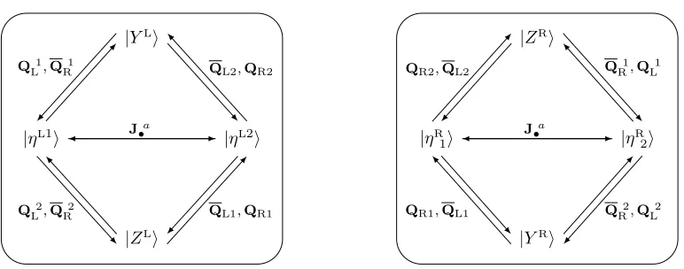
3.2.1 Left representation
One representation of dimension four (two bosons and two fermions) has eigenvalue +1 under M, and consists only of excitations labelled “L”. These correspond to half of the transverse modes on AdS3×S3, and it can be represented as in the left panel of figure1. This is a bi-fundamental representation ofpsu(1|1)4c.e., supplemented by the action ofsu(2)• on the fermions. In particular, the fermions are in the fundamental representation
J•a˙b˙|ηLc˙i=−δ c˙
a |ηL
˙
bi+1 2δ
˙
b
˙
a |ηLc˙i. (3.20)