Theses
Thesis/Dissertation Collections
2012
Signal to noise ratio estimation using the
Expectation Maximization Algorithm
Ahmed Almradi
Follow this and additional works at:
http://scholarworks.rit.edu/theses
This Thesis is brought to you for free and open access by the Thesis/Dissertation Collections at RIT Scholar Works. It has been accepted for inclusion in Theses by an authorized administrator of RIT Scholar Works. For more information, please [email protected].
Recommended Citation
By
AHMEDMALMRADI
A Thesis is submitted in partial fulfillment of the requirements for the degree of
MASTEROFSCIENCEinElectricalEngineering
APPROVED BY:
………
Dr. Sohail Dianat, Thesis advisor
………
Dr. Ernest Fokoué, Thesis Committee member
……….
Dr. Chance M. Glenn, Thesis Committee member
……….
Dr. Vincent Amuso, Thesis Committee member
……….
Dr. Sohail Dianat, Department head
DEPARTMENT OF ELECTRICAL AND MICROELECTRONIC ENGINEERING
KATE GLEASON COLLEGE OF ENGINEERING
ROCHESTER INSTITUTE OF TECHNOLOGY
By:
AHMEDALMRADI
Thesisadvisor:
Dr.SOHAILDIANAT
Abstract
TABLEODCONTENTS
List of figures . . . . . . . iv
List of symbols and abbreviations . . . . . . . v
Acknowledgments. . . . viii
Abstract . . . . . ix
1. Introduction . . . . 1
1.1 Estimation. . . . 2
1.2 Multivariate Gaussian distribution. . . . . 5
1.3 Minimum Variance Unbiased Estimator (MVUE) . . . . . . . 7
1.4 Cramer Rao Lower Bound (CRLB) . . . .. . . . . 8
2. Mixtures of Gaussians (MoG) . . . . . . . . 10
2.1 The Basic definition of MoG. . . . . . . 10
2.2 The Likelihood function. . . . 12
3. The EM algorithm. . . 15
3.1 Introduction. . . . . . . 15
3.2 Jensen’s Equality. . . 16
3.3 Kullback‐Leibler (KL) Divergence. . . . . . . . 17
3.4 The EM Derivation. . . . . 18
3.5Mixture of Gaussians and the EM algorithm. . . . 22 4. SISO NDA SNR estimation using the EM algorithm in the Literature . . . . . . . . . . . . 27
4.1 The BPSK case. . . . . . . . . . . . 27
4.1.1 The system model. . . . . . . . 27
4.2 The QPSK case. . . . . . . . . . . . 38
4.2.1 The CRLB for QPSK. . . . . . . . . . . . . . . . 41
4.2.2 SISO NDA SNR estimation using the EM algorithm for the QPSK case . . . . 43
5. MISO with STBC NDA SNR estimation using the Expectation Maximization algorithm . . . . . 51
5.1 Conventional Receive diversity (SIMO) model. . . . . . . . . 51
5.2 Transmit diversity (MISO) model. . . . . . . . 52
5.3 MIMO model. . . . . . . . . . . . . . . . 53
5.4 The transmit diversity for BPSK case. . . . . . . . . . . . . . . . 54
5.5 The CRLB for the transmit diversity in the BPSK case. . . . . . . . . . 58
5.6 STBC NDA SNR estimation using the EM algorithm. . . . . . . . . 65
6. Conclusions . . . . . . . . . . . . . . . . . . . 70
7. Future work . . . . . . . . . . . . . . . . . . 70
LISTOFFIGURES
Figure 1.1 Normal distribution with 0 and 1 . . . 3
Figure 2.1 Mixtures of two Gaussians . . . 11
Figure 2.2 Samples and their contour of the previous distribution . . . 11
Figure 3.1 mixtures of four Gaussians data and their fit when C 0.35I . . . . . . . . . 26
Figure 3.2 mixtures of four Gaussians data and their fit when C 0.05I . . . . . . 26
Figure 4.1 The MSE & CRLB in dB2 vs. SNR in dB for the BPSK when N=128 . . . . 35
Figure 4.2 The MSE & CRLB in dB2 vs. SNR in dB for the BPSK when N=512 . . . 36
Figure 4.3 The MSE & CRLB in dB2 vs. SNR in dB for the BPSK when N=1024 . . . . 37
Figure 4.4 The Error in dB2 vs. SNR in dB for BPSK at different Ns . . . 37
Figure 4.5 The MSE in dB2 vs. N. . . . . . 38
Figure 4.6 The MSE & CRLB in dB2 vs. SNR in dB for the QPSK when N=128 . . . 47
Figure 4.7 The MSE & CRLB in dB2 vs. SNR in dB for the QPSK when N=512 . . . . 48
Figure 4.8 The MSE & CRLB in dB2 vs. SNR in dB for the QPSK when N=1024 . . . . 49
Figure 4.9 The Error in dB2 vs. SNR in dB for QPSK at different Ns . . . 49
Figure 5.1 SIMO/ Receive diversity system model . . . . . . . . 51
Figure 5.1 MISO/ Transmit diversity system model . . . 52
Figure 5.3 MIMO system model . . . . . . 53
Figure 5.4. The MSE & CRLB in dB2 vs. SNR in dB for STBC when N=128 . . . 67
Figure 5.5. The MSE & CRLB in dB2 vs. SNR in dB for STBC when N=512 . . . 67
LISTOFSYMBOLSANDABBREVIATIONS
Symbols
Signal to Noise Ratio in dB
Estimated Signal to Noise Ratio in dB Non Data Aided
Data Aided
Binary Phase Shift Keying Quadrature Phase Shift Keying Expectation Maximization
. . . Independent and Identically Distributed Cramer Rao Lower Bound
Additive White Gaussian Noise Maximum Likelihood
Single Input Single Output Single Input Multiple Output Multiple Input Single Output
Multiple Input Multiple Output Space‐ Time Block Codes
Minimum Variance Unbiased Estimator Mixtures of Gaussians
Monte Carlo
Probability Density Function
Ө Parameters which need to be estimated Ө The Estimated parameter Values
μ , ∑ Real Gaussian distribution with mean μ and Covariance ∑ μ , ∑ Complex Gaussian distribution with mean μ and Covariance ∑ Ө Likelihood function
Ө Log Likelihood function
Gradient with respect to the parameters Real of
Imaginary of μ Mean
Variance
μ Estimated mean Estimated variance The Expected value
Ө Fisher Information Matrix
Ө Element ij of the Fisher Information Matrix
Mean Square Error Ө Bias
Acknowledgments
I introduce my deep gratitude to my advisor, Dr. Sohail Dianat, for his constant guidance and support till we made this work visible and valuable. His vision and ideas make mine grow gradually during my work in finishing this project. I am thankful for the opportunity in being under his guidance and support.
I also would like to send my thanks to Dr. Ernest Fokoue, from the center for quality and applied statistics, for his appreciated and valuable discussion which helped me shape my project in a better way. His knowledge filled in the gap which I had in some statistical concepts regarding density estimation when incomplete data is present.
Abstract
Signal to Noise Ratio (SNR) estimation when the transmitted symbols are unknown is a common problem in many communication systems, especially those which require an accurate SNR estimation. In this study, Non data Aided (NDA) SNR estimation for Binary Phase Shift Keying (PBSK) and Quadrature Phase Shift Keying (QPSK) using the Expectation Maximization (EM) algorithm is developed. The assumption here is that the received data samples are drawn from a mixture of Gaussians distribution and they are independent and identically distributed . . . . The quality of the proposed estimator is examined via the Cramer‐Rao Lower Bound (CRLB) of NDA SNR estimator. It is also assumed that the channel gain is constant during each symbol interval, and the noise is Additive White Gaussian (AWGN). Maximum Likelihood estimator is being used if we have access to the complete data, in this case the problem would be much easier since we get the exact closed form solution, but when the observed data are incomplete or partially available, the EM algorithm will be used. This approach is an iterative method to get an approximated result which is either an approximated global maximum or local maximum. However, in the NDA SNR estimation, we only have a global maximum since our assumption is that the distribution is a mixture of Gaussians. This is being investigated for the cases of Single Input Single Output (SISO); [3], [4], [10], and Single Input Multiple Output (SIMO); [5], [9]. The main concern about the receive diversity is the cost, size, and power, that is why we resort to the transmit diversity such as Multiple Input single Output(MISO) with space time block codes (STBC). The base station usually serves hundreds to thousands of remote units which is the sole reason of using transmit diversity at the base station instead of at every remote unit covered by the base station. It is more economical in this case to add equipments to the base station instead of the remote units. Alamouti [12] used a simple transmit diversity technique and assumed in his paper that the receiver has perfect knowledge of the channel transition matrix. However, this assumption may seem highly unrealistic. One of our contributions is to estimate the channel information, as well as the noise variance which would be used in estimating the SNR and deriving the CRLB for both DA and NDA case. The performance of our estimator would be empirically assessed using Monte‐Carlo simulations, with CRLB as a performance metric.
1Introduction
Many modern wireless communication systems require the Signal to Noise ratio (SNR) estimation without the knowledge of the transmitted data symbols in Non‐Data Aided (NDA) manner. SNR estimators may be divided to two categories, Data Aided (DA) and Non Data Aided (NDA). In DA estimators, the transmitted symbols are used or known at the receiver and used in the estimation process, in NDA estimators; the estimation process is being done without the knowledge of the transmitted symbols, just based on the received samples. The Cramer‐Rao Lower Bound (CRLB) for NDA SNR estimation, which gives the minimum variance of unbiased estimators, will be used in evaluating our estimator [5]. The CRLB for NDA SNR estimation for the BPSK and QPSK will be derived and plotted against the EM‐ML NDA SNR estimator. Here, the transmitted symbols are treated as unknown parameters, but nuisance parameter; unknown and unwanted. This estimation procedure would be close to the CRLB for the SNR of interest; at sufficiently high SNR. The main purpose of this study is to derive a closed form approximation for the NDA CRLB in the BPSK and QPSK case. Besides, the derivations of the EM algorithm for NDA SNR estimation which will iteratively maximize the likelihood function till reach approximately the global maximum.
1.1Estimation
The problem of parameter estimation is a common problem that is widely faced in many areas such as Radar, speech, image analysis, biomedicine, communications, control, and much more. The problem we are faced with is estimating some parameters based on some seen or observed samples due to the use of digital communication systems or digital computers [2]. Mathematically, we
observe N data points at the receiver side 1 , 2 , . . . , N which sampled from an unknown
probability density function ; Ө parameterized by an unknown parameter Ө, which is the parameter of interest. Unfortunately, we don’t really get to see the distribution of the received sample Y. We only get that sample, Y, which we then use to estimate our parameter Ө. As a result of that, our estimator won’t give us the exact Ө, but an estimated version of it. Our estimator will depend highly through some function of the received sample Y as,
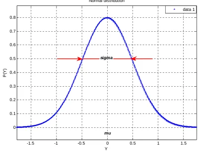
Ө 1 , 2 , . . . , N 1.1 This estimator might be used to estimate the carrier frequency, channel phase, signal power, noise power,….etc. Since the received data are random, we can describe its behavior according to its PDF function, 1 , 2 , . . . , N ; Ө . The semicolon is used to indicate that the distribution of PDF is parameterized by the parameter Ө. And it is constant. This kind of estimation is called classical parameter estimation because the parameters of interest are assumed to be deterministic and needs to be estimated. Since we are assuming the noise which corrupted our received signal is additive white Gaussian noise, AWGN, the distribution of the PDF of the received samples will be Gaussian distribution. For example, if we received one sample and the parameter which needs to be estimated is the mean and variance. Figure 1.1 shows a normal distribution of zero mean and unite variance. This is just an illustrative example which shows us the parameters which we will be estimating. Assume that we have a signal which happen to be constant corrupted by AWGN, w(n), our model will be as follows,
μ
The parameters which need to be estimated here are two, the DC component or average, and the variance of our Gaussian noise.
If one sample has been observed,
Figure 1.1 Normal distribution with mu=0, sigma=1
Ө μ
then,
1 ; Ө 1
√2
1 μ
2 1.2
The assumption is that the noise 1 ~ 0, . Or in general, each sample of has the same
PDF as 1 . Since these samples are uncorrelated with each other, uncorrelated means
independent if the distribution is Gaussian, we can now generalize the PDF of the received samples Y of size N as follows,
1 , 2 , . . . , N ; Ө ; Ө ; Ө Ө/
-1.5 -1 -0.5 0 0.5 1 1.5
0 0.1 0.2 0.3 0.4 0.5 0.6 0.7 0.8
Normal distribution
Y
P(
Y)
data 1
1 √2
n μ
2
1 2
1
2 n μ 1.3.1
Equation (1.3) is called the likelihood function of the received data, which would be used to find the Maximum Likelihood estimate (MLE) of the mean and variance in case of our received data were generated by single Gaussian. I just wanted to make this clear because in the next chapter we will be talking about received sample which has been generated by more than one Gaussian; Mixture of Gaussians. To find the MLE of equation (1.3), we need to find the values of μ and which
maximizes the likelihood function Ө .We can instead maximize the log likelihood function since
the logarithm is a monotonic function. MLE has the asymptotic property of being unbiased. It is also proved that MLE achieves the CRLB for high SNR.
Ө
2 2
1
2 n μ 1.3.2
Ө
Ө
Ө
which can be found by setting the gradient of
Ө with respect to
Ө equal to zero;Ө Ө 0.
The ML solution is given as,
μ 1 1.4
1
μ 1.5
μ 1
μ μ 1.6
1
μ
1 2 1
1
1.7
So, we see that the MLE of the variance is biased, while the MLE of the mean is unbiased. The MLE distribution may be approximated as,
Ө ~ Ө, Ө 1.8
Where, ~ asymptotically distributed according to, Ө is the fisher information which is given by,
Ө ; Ө
Ө 1.9
A computer simulation could be performed to define how large the data length N had to be in order to get this asymptotic result. Monte Carlo method could be used for various realizations (say M) of our estimate Ө , The mean and variance of the estimator could then be calculated as,
Ө 1 Ө 1.10
Ө 1 Ө Ө 1.11
1.2MultivariateGaussiandistribution
Since the focus on this research will be on Gaussian distribution, it is worth introducing the general multivariate Gaussian distribution, its behavior and properties.
Suppose we have a random variable that follows a multivariate Gaussian distribution. This random variable may be signal corrupted by noise.
…
; μ …
Its covariance matrix is; ∑ Y μ Y μ
Then, the distribution of this random variable will be given by,
1
|2 ∑ |
1
2 μ ∑ μ 1.12
If the Covariance matrix ∑ , independent random variables with equal variances, each of the
received samples dimension in equation (1.12) will return to equation (1.2). Let us mention an important property which is the effect of linear transformation on Gaussian distribution, let,
where, A and b are constants matrix and vector respectively, and X is a vector of random variable.
, μ μ
, ∑ ∑
The MLE in the multivariate case would be as follows, the model parameters which need to be estimated is,
Ө μ ∑ , assuming i.i.d samples,
; Ө 1
|2 ∑ |
1
2 μ ∑ μ
|2 ∑ | 1
Ө ; Ө
2 |2 ∑ |
1
2 μ ∑ μ
To find the MLE of this parameter, we need to go through the same process of differentiating the likelihood of equation (1.12) and equating it to zero we get the following,
Ө
Ө , first we differntiate with respect to μ as
Ө
μ , we get,
μ 1 1.13
and differntiating with respect to the covariance matrix Ө
∑ , we get,
∑ 1 μ μ 1.14
The parameter estimate in this case is straight forward computed in a closed form since the assumption that Y’s samples are being drawn from only one Gaussian distribution. However, this won’t be the case when we have a mixture of Gaussians. The proposed algorithm will be a mixture of multivariate Gaussian distribution since we are dealing with PBSK and QPSK constellation systems and the transmitted data symbols are unknown.
1.3MinimumVarianceUnbiasedEstimator(MVUE)
The search for good estimators of unknown deterministic parameters isn’t always an easy task. Our focus will be on estimators which on average yield the true parameter value, and then among all those estimators, we look for the one which has the least variance. For an estimator to be unbiased,
Ө Ө 1.15
The bias of an estimator may be defined as,
Ө Ө Ө 1.16
Ө Ө Ө 1.17
Good estimators have small MSE or small variance if the bias is zero. Equations (1.16) and (1.17) are unrealizable estimators since they are function of the true parameter value, so we cannot assess the performance of the estimator in this case.
MSE is composed to error due to the bias and variance. MVUE does not always exist, and if it did, sometimes it is not easy to be found [2]. One way of finding it is using the Cramer Rao Lower Bound
(CRLB). When CRLB satisfies with equality for all Ө,the .
1.4CramerRaoLowerBound(CRLB)
Finding a lower bound on the variance of an unbiased estimator will be extremely important in practice. This will serve as a benchmark in comparing the goodness of an estimator. CRLB allows us to assure that an estimator is the minimum variance unbiased estimator (MVUE), which will be the case when the estimator attains the CRLB for all values of the unknown parameter.
If ; Ө satisfies regularity conditions, the variance of unbiased estimator is defined as,
Ө 1 ; Ө
Ө
1.18
An estimator may be found that attains the bound for all Өifand only if the score function can be written as,
; Ө
Ө Ө Ө
For some functions g and I, that estimator which is the MVUE is given by,
Ө
And the minimum variance is
Ө 1
Then this estimator is said to be efficient.
Let us extend the CRLB to a vector parameter,
Ө Ө Ө Ө … Ө
Ө Ө 1.19
where Ө is the Fisher information matrix.
Ө ; Ө
Ө Ө 1.20
For example if
Ө μ
Then,
Ө
; Ө μ
; Ө μ
; Ө μ
; Ө
This matrix is symmetric and positive definite.
If we are estimating a function of the parameter as in the research study, if
Ө
Then,
Ө
Ө Ө
2 MixturesofGaussians(MoG)
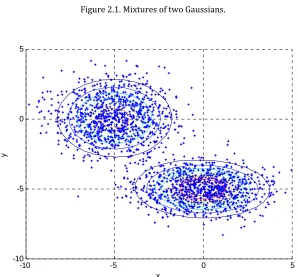
When it is not possible for one Gaussian distribution to represent our model, we resort the mixture of Gaussians method. It is a combined (mixture) of some known distributions that are combined to form our model. In our estimation problem, our assumption is that we are given a received samples Y of length N, which are drawn from a mixture of Gaussians distribution. The number of Gaussians is determined by the constellation order we use. For example, in PBSK, we have two mixtures of Gaussians per antenna with means {‐1, +1}, and in QPSK, we have four mixtures of Gaussians per
antenna with means {
√ , √ }. Gaussian Mixture Model (GMM) can be used in modeling
complicated probability density functions (PDFs) which have complicated shapes that cannot be modeled using a single Gaussian.
2.1ThebasicdefinitionofMoG
The general form of a Gaussian mixture models is
/Ө , /Ө
/ , Ө
; μ , ∑ 2.1
where is the component prior of each Gaussian component. There is a necessary condition for
to be a valid probability density function that, ∑ 1 and 0. The parameters
Figure 2.1. Mixtures of two Gaussians.
Figure 2.2. Samples and Contours of the previous distribution.
-10
-5
0
5
10
-10 -5 0 5 10
0 0.01 0.02 0.03 0.04 0.05
x Mixture of two Gaussians
y
p
(x,
y)
-10 -5 0 5
-10 -5 0 5
x
2.2TheLikelihoodfunction
The likelihood function is a function of the parameters of a statistical model given the observation data. The maximum likelihood solution selects values for the model parameters that give a distribution which gives the observed data the highest probability. Let us introduce the Maximum Likelihood estimate (MLE) of a Gaussian Mixture Model (GMM). Maximizing the likelihood function is the same as maximizing the Log Likelihood function since the likelihood function is a monotonic function. This, in the case of one Gaussian or when there is no hidden variables would simplify the math a lot since the likelihood function is exponential function, so the log function will cancel the exponential and we would be left with the exponent. The Log likelihood function for the data is given by,
Ө /Ө
/ , Ө
; μ , ∑ 2.2
Where, it is clear here that the likelihood function depends on the PDF at a given mixture
component. In the estimation problem we’ve assumed that the noise is AWGN, so ∑ ,but
∑ in general may take any covariance matrix form. Therefore the log Likelihood function becomes,
Ө
2
‖ μ ‖
2 2.3
Ө
Ө Ө
2.4
This may be solved by differentiating the log Likelihood function and equate it to zero as follows,
Ө Ө ,
Ө
Ө /Ө
/ , Ө
Ө 0
Where, Ө μ , ∑ in the Gaussian distribution case, the distribution of interest,
Let us first let Ө μ then,
Ө μ
/μ , ∑
∑ /μ , ∑ ∑ μ 0
, / , Ө /μ , ∑
∑ /μ , ∑
, μ ∑∑ / , Ө
/ , Ө 2.5
Similarly, let Ө ∑ then,
Ө
∑ ∑ /μ , ∑
/μ , ∑
∑ 0
Ө
∑ ∑ /μ , ∑
1
2 /μ , ∑ ∑ μ ∑ μ ∑
, ∑ ∑ / , Ө μ μ
∑ / , Ө 2.6
We conclude that μ , ∑ estimates will only be correct when using the correct posterior
distribution / , Ө , but the posterior distribution / , Ө depends on them both. So,
there is no compact form solution for these parameters. We then turn to an iterative solution to finding the maximum likelihood estimate which will be our target in this research where we will be using the Expectation Maximization as an iterative approach in finding the Maximum Likelihood solution.
Ө, /Ө 1
Then now differentiate this function, Ө, ,with respect to both, the mixing coefficients, , and
the Lagrange multiplier, , we get the estimated mixture component as below,
1
N / , Ө 2.7
3 TheExpectationMaximization (EM)Algorithm
3.1Introduction
This is for discrete random variables, the same is true when working with continuous random variables except switching the summation in equation (3.1) in to integration over the latent variable Z. The bad news here in equation (3.1) is that the summation over the latent variable Z is inside the logarithm which made it clear that the solution of this equation won’t be an easy task. We can see that since the logarithm and exponentials won’t be canceled with each other as we’ve seen in the previous chapter. In the previous chapter the summation was outside the logarithm which made it easy to be cancelled with the exponential of the Gaussian distribution. Let us assume that for every observed sample in Y, we know the corresponding latent variable Z. Then we can call , as the complete data set. We will refer to Y as incomplete data.
Maximization of the complete data log likelihood function , is straight forward done
by MLE. However, we don’t really get to see the latent variables Z, but only the incomplete data
Y. we know Z by the posterior distribution / , Ө . Since we cannot use the complete data log
likelihood, we instead take its expected value under the posterior distribution of the latent variable. This step corresponds to the E step of the EM algorithm. The M step then would be maximizing this expectation with respect to the parameters of interest. If we denote the current
estimate as Ө , then the E and M steps would result in a better estimate Ө . These two steps
will then be repeated till we get some precision degree [1]. We start our EM algorithm by choosing an initial point Ө for the parameters to start with. In the E step, we use the current
parameter value Ө to find the posterior distribution of the latent variables / , Ө . We then
use this posterior distribution in finding the expectation of the complete data log likelihood
computed at Ө , we denote this expectation as Ө , Ө , which called auxiliary function,
is given by,
Ө , Ө / , Ө , /Ө 3.2
Ө is then computed in the M step as,
Ө
Ө Ө , Ө 3.3
Let us prove those equations alongside with the convergence of the EM algorithm regardless of any initial starting point. To do that, we need to introduce some definitions.
3.2Jensen’sInequality
3.4
Where f is any concave function and ∑ 1, and 0 1.
Also,
or,
1 1
3.3Kullback‐Leibler(KL)Divergence
This helps us find the divergence between two probability distribution functions. Let us take two distributions, p(y) and q(y). Then the KL divergence between them is given by,
,
Using the fact that 1, we then get,
1
0
Then we see that , 0.
This gives the following,
Let us try to write the KL divergence in the case of two Gaussians,
Let, ; μ , ∑ and, ; μ , ∑ then,
, 1
2 ∑ ∑ μ μ ∑ μ μ
|∑ |
|∑ | 3.6
3.4TheEMDerivation
If we consider a mixture of Gaussians distribution, the parameters values which need to be
estimated are the means, , , . . , covariances, ∑ , ∑ , … , ∑ and component priors,
, , … , . Those values will change from iteration to iteration, Ө to Ө till they reach the
optimum value or stabilize at some values. Once the Ө goes to Ө , the PDF will also iterate from
/Ө to /Ө . The increase in the log likelihood will be,
Ө Ө /Ө /Ө
/Ө
/Ө 3.7
In the case of mixture model, we need to introduce the latent variables as being one of the M mixtures.
Ө Ө 1
/Ө , /Ө
1 /Ө
/ , Ө , /Ө
/ , Ө
Since the log function is strictly concave, we can apply Jensen’s Inequality as follows,
Ө Ө / , Ө , /Ө
/Ө / , Ө 3.8
Also, we’ve seen from (3.2) that the auxiliary function may be written as,
Ө , Ө / , Ө , /Ө
We can then rewrite equation (3.7) as,
Ө Ө Ө , Ө Ө , Ө
The difference in the auxiliary function gives a lower bound on the increase in the log likelihood. We can see that Ө , Ө depends on the current parameters, so if we just maximize the auxiliary
function Ө , Ө , the likelihood function will also be maximized as a result of that. Now our
aim is to maximize the function Ө , Ө to get to the parameters of interest. We can do that by
differentiating the auxiliary function Ө , Ө with respect to the new parameters Ө and
equate the result to zero. We need to make sure that when maximizing the function with respect to the mixing proportion, we need to use Lagrange multiplier.
Ө Ө , Ө 0.
What we need to guarantee is that as we iterate from Ө to Ө , we need to make sure that we are
in fact increasing the log likelihood function or else we are not improving or going towards the optimum solution. We need,
Ө Ө or,
Ө Ө 0.
Let us introduce the posterior distribution of the latent variable / , Ө ,
/Ө /Ө / , Ө /Ө /Ө
Since,
/ , Ө 1
/Ө , /Ө / , Ө
We can then write the following,
/ , Ө /Ө / , Ө , /Ө
/ , Ө
Similarly for the second term,
/ , Ө /Ө / , Ө , /Ө
/ , Ө
Combining the last two equations we get,
Ө Ө / , Ө , /Ө / , Ө / , Ө
/ , Ө , /Ө / , Ө / , Ө
From the definition of the KL divergence,
/ , Ө , / , Ө / , Ө / , Ө
/ , Ө 0
Using this KL divergence equation in the last equation we get,
Ө Ө / , Ө , /Ө / , Ө , /Ө
Where, the difference between the left and right hand sides is the KL divergence. If we can assure that the right hand side is positive, then the left hand side will be also positive.
Suffices to show that,
/ , Ө , /Ө / , Ө , /Ө
Which will assure that,
Let us recall the auxiliary function,
Ө , Ө / , Ө , /Ө
If the auxiliary function increases, then the likelihood will also increase. If,
Ө , Ө Ө , Ө
Then,
Ө Ө .
We can see the difference between the likelihoods and the auxiliary functions would be the KL divergence, as follows,
Ө Ө Ө , Ө Ө , Ө / , Ө , / , Ө 3.9
The increase in the auxiliary function would be a lower bound on the increase of the log likelihood. We noted that maximizing the auxiliary function once, doesn’t result in the optimum parameter values, we need to iterate till convergence is being achieved. We can now summarize the EM algorithm in two steps:
⤇ The Expectation step which is done after guessing a starting point Ө and calculating the posterior distribution of the latent variable, / , Ө , by taking the expected value of the log
likelihood of the complete data in terms of the new parameter values Ө , , /
Ө , Ө with respect to the posterior distribution of the latent variables , / , Ө . As
follows,
Ө , Ө / ,Ө , /Ө , Ө 3.10
⤇ The Maximization step which maximizes the auxiliary function, Ө , Ө , with respect to the
new parameters Ө .
Ө
Ө Ө , Ө
the global maxima. One way of trying to overcome this problem is by starting at many different initial points and then chooses the one which gives the highest likelihood.
3.5MixtureofGaussiansandtheEMalgorithm
One of the applications of the EM algorithm is to find the MLE of the Mixture of Gaussians parameters in the existing of unobserved variables or data. We’ve seen that the parameters couldn’t be found by a direct MLE. An iterative procedure needs to be done in order for us to get to the optimum results for the parameters. The major problem which we encounter here is that which Gaussian component was responsible for generating that specific sample. We know that the latent variables are discrete which determines the number of mixtures which have been used in generating the observed data. If we have prior knowledge about the components which were responsible for generating the data, then the problem would become easier and could be solved using a direct MLE. So now our major problem is estimating the component which was responsible for generating each data point in my observed data. Once we know the posterior distribution of the hidden variables / , Ө , the problem then become like a direct MLE problem in the auxiliary function sense.
Assume that, 1 if the observed data was generated by component
0 otherwise
Let us have a look at a single received sample which we suppose that it was generated by
component . We can write,
, /Ө / , Ө
/ , Ө 3.11
In addition of Y being . . . samples, Z also are . . . samples,
, /Ө , /Ө
Ө , Ө / , Ө , /Ө
/ , Ө , /Ө
/ , Ө , /Ө
/ , Ө , /Ө
/ , Ө / , Ө
/ , Ө / , Ө
/ , Ө
Ө , Ө / , Ө / , Ө
/ , Ө 3.12
We know that the log likelihood function for a component mixture is,
; μ , ∑ 1
2 2 |∑ | μ ∑ μ
Ө , Ө / , Ө 1
2 μ ∑ μ
/ , Ө 1
2 2 ∑
/ , Ө 3.13
We now need to estimate the parameters of interest of component at iteration 1 by differentiating the auxiliary function with respect to one of the parameters and equating to zero,
Ө Ө , Ө 0
In the case of estimating the mean of the mixture component,
Ө , Ө 0
This will result in the updating mean formula,
μ ∑ / , Ө
∑ / , Ө 3.14
∑ Ө , Ө 0
This will result in the updating Covariance formula,
∑ ∑ / , Ө μ μ
∑ / , Ө 3.15
Equations (3.13) to (3.15) will be iterated till convergence is achieved.
To sum up, the EM algorithm for Mixture of Gaussians may be summarized as follows,
1. Initialize the parameters mean μ , Covariance ∑ , and mixing coefficient , then calculate the initial value for the log likelihood function.
2. In the E step, we need to calculate the responsibilities, / , Ө ,
/ , Ө ∑ /μ , ∑
/μ , ∑
∑ / , Ө
∑ / , Ө
∑ ∑ / , Ө
∑ / , Ө
∑ / , Ө
4. Evaluate the log likelihood checking for increasing the log likelihood and stopping the iteration process if a given precision has been achieved.
/ , , ∑ /μ , ∑
If the precision hasn’t been achieved, we go back to point number 2 and iterate once again. We do the same procedure till we achieve the precision condition.
For instance, let us consider an example showing a mixture of four Gaussians as an illustration example. I assumed that the means as the values of the four sent symbols in the
QPSK case, ∈ 1 , 1 , and have equal covariance of ∑ 0.35 , where I is a 2×2 matrix.
Figure 3.1 shown shows these generated data with its Gaussian fit using the previous algorithm, my assumption model was like,
Where is the received data which corrupted by additive white Gaussian noise AWGN, of
covariance,∑,both of size N, and 1, 1 . This is done by generating 800 samples
Figure 3.1. mixtures of four Gaussians data and their fit when 0.35
Figure 3.2. mixtures of four Gaussians data and their fit when 0.05
-2.5 -2 -1.5 -1 -0.5 0 0.5 1 1.5 2 2.5 -2.5 -2 -1.5 -1 -0.5 0 0.5 1 1.5 2
y1(n)
y2
(n
)
-2.5 -2 -1.5 -1 -0.5 0 0.5 1 1.5 2 2.5 -2.5 -2 -1.5 -1 -0.5 0 0.5 1 1.5 2
y1(n)
y2
(n
)
-3 -2 -1 0 1 2 3
-4 -3 -2 -1 0 1 2 3 4 y 1(n) y2 (n ) Cluster 1 Cluster 2 Cluster 3 Cluster 4 C o m p o n e n t 1 P o s te rio r P ro b a b ilit y 0.1 0.2 0.3 0.4 0.5 0.6 0.7 0.8 0.9
-3 -2 -1 0 1 2 3
-3 -2 -1 0 1 2 3 y 1(n) y2 (n)
partitioned data using the K-means Cluster 1 Cluster 2 Cluster 3 Cluster 4 Centroids
-2 -1.5 -1 -0.5 0 0.5 1 1.5 2 -2 -1.5 -1 -0.5 0 0.5 1 1.5 2 y 1(n) y2 (n) Cluster 1 Cluster 2 Cluster 3 Cluster 4 C o m p o n e n t 1 P o s te rio r P ro b a b ilit y 0 0.1 0.2 0.3 0.4 0.5 0.6 0.7 0.8 0.9 1
-2 -1.5 -1 -0.5 0 0.5 1 1.5 2 -2 -1.5 -1 -0.5 0 0.5 1 1.5 2
y1(n)
y2
(n
)
partitioned data using the k-means Cluster 1 Cluster 2 Cluster 3 Cluster 4 Centroids -2 -1.5 -1 -0.5 0 0.5 1 1.5 2 -2 -1.5 -1 -0.5 0 0.5 1 1.5 2
y1(n)
y2
(n
)
Scatter plot with noise Covariance 0.05I
-2.5 -2 -1.5 -1 -0.5 0 0.5 1 1.5 2 2.5
-2.5 -2 -1.5 -1 -0.5 0 0.5 1 1.5 2 2.5
y1(n) y2
(n
)
4 SISONDASNRestimationusingtheEMalgorithmintheLiterature
4.1BPSKcase
In the binary phase shift keying, we have a mixture of two classes, ∈ 1, 1 . Those are the transmitted symbols.
4.1.1 Thesystemmodel
We are assuming that there is no error in timing, phase deviation, or frequency deviation. The matched filter output may be given by,
, 1, … . . , 4.1
where, is the received sample, is the transmitted symbol, is the channel gain, and is a
zero mean AWGN with variance .
We can write equation (4.1) in a vector form as,
4.2
where, . . . . , . . . . , . . .. . The transmitted
symbols may be modeled as realizations of . . . binary random variables. The probability distribution function may be written as,
/ , Ө 1
√2 2 4.3
Assuming equally likely symbols, we have,
; Ө / , Ө /Ө
1 √2
1
2 2
1
2 2
where, Ө . Now for N received . . . samples we have,
; Ө 1 √2
1
2 2 2 4.4
This is the likelihood function of the received data. Now given the observation data, estimate the
parameter values Ө and then substitute to find the SNR,
10
4.1.2 TheCRLBforBPSK
The Cramer‐Rao Lower Bound (CRLB) is a lower bound for the Mean Square Error (MSE) of any unbiased estimator which satisfies the regularity condition [2]. In our case of SNR estimation, the CRLB can be written as,
Ө Ө Ө 4.5
Where Ө is the fisher information matrix given by,
Ө
; Ө ; Ө
; Ө ; Ө 4.6
And,
Ө
20 10
10
10 4.7
FortheNDAcase,
The log likelihood function is given as,
Ө /Ө
2 2
1
After differentiating this function with respect to the channel gain and the variance we get the following,
; Ө
; Ө
; Ө ; Ө
; Ө 2
1 2
Ө
1
1 2
4.9
where,
2 √2
2
4.10
We can now substitute this result into equation (4.5) and get the following,
20 10
10 10
1
1 2
20 10 10
10
200 10
2 1
FortheDAcase,
Ө / , Ө
1
2 2 2
where is given to be either +1 or ‐1.
After differentiating this function with respect to the channel gain and the variance we get the following,
; Ө
; Ө
; Ө ; Ө
; Ө 2
1
Ө 0
0 2
4.12
We may now substitute this result into equation (4.5) and get the following,
20 10
10 10
0
0 2
20 10 10
10
200
10
2
4.1.3 NDASNRestimationusingtheEMalgorithm
We now introduce the method of EM algorithm in estimating the SNR. Our assumptions are that the data was drawn from a mixture of two Gaussians, and are uncorrelated with each other. The samples are drawn in an . . . manner. The parameters which we need to estimate now are,
Ө
Ө
; Ө
10 4.14
The EM algorithm will be used to iteratively estimate the channel gain and the noise variance then use them to estimate the signal to noise ratio. The received data will be seen as incomplete data set since we don’t know its class (transmitted symbol). The auxiliary function in this case may be given as,
Ө , Ө / ,Ө , /Ө , Ө
Ө , Ө / , Ө / , Ө
/ , Ө 4.15
Ө
Ө
Ө , Ө
4.16
Now solving those two equations will give us the E & M steps. Since we know the mixing
proportion , we don’t need to estimate it.
The auxiliary function may be given as,
Ө , Ө / , Ө 1
2 ∑
/ , Ө 1
2 2 ∑ / , Ө
/ , Ө 1
2 2 2
Ө , Ө
/ , Ө
2 0
/ , Ө 0
/ , Ө 0
/ , Ө
/ , Ө / , Ө
, / , Ө / , Ө 1
/ , Ө 1 / , Ө
2 / , Ө 1
1
2 / , Ө 1 2 2
2 2
1
2
2 2 2
2 2
2 2
2 2
1
4.17
Solving for the variance, we have,
Ө , Ө
/ , Ө / , Ө / , Ө / , Ө 0
/ , Ө 1
2 2 / , Ө
1
2 2 0
/ , Ө 1
2 2 1 / , Ө
1
2 2
0
/ , Ө
2
1
2 / , Ө 1
2 2 0
4 / , Ө 2 0
2 2 / , Ө 1 0
2
2 0
2 0
1
4.18
10
1
4.19
1
4.20
estimate the signal to noise ratio, , as given above. The will be found for different
estimated values of SNR. Then this MSE will be assessed using the NDA CRLB in units of dB2. The
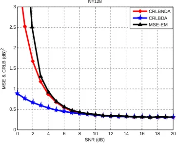
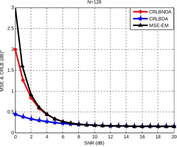
[image:46.612.118.481.363.658.2]estimation process will be done for a range of SNR from 1 dB to 20 dB, and for different values of received sample size, N, 128, 512 and 1024. Figure 4.1 shown explains three things when BPSK is used as the transmitted symbols. The red curve is the CRLB for NDA signal, the blue curve is the CRLB for DA signal, and the black curve shows the MSE estimated using the EM algorithm. The EM algorithm estimate is repeated 10000 times using Monte Carlo simulations to get 10000 realizations of the SNR estimates, then averaging them to get the estimated SNR, then finding the variance to get the MSE for that specific SNR estimate value. We then repeat this process for different values of SNR, say from 0 dB to 20 dB and their resultant MSE. Those estimates then assessed with the CRLB as shown below. We see that for low SNR estimate values, the MSE is large compared with the NDA CRLB. The higher the SNR become, the lower the MSE we get till they (the CRLB and MSE) both match. This was for sample size of N=128. The next step we would do is increase N and see what is going to happen to our estimation accuracy.
Figure 4.1 The MSE & CRLB in dB2 vs. SNR in dB when N=128 for the BPSK case
0 2 4 6 8 10 12 14 16 18 20
0 0.5 1 1.5 2 2.5 3
SNR (dB)
M
S
E
& C
R
L
B
(
d
B)
2
N=128
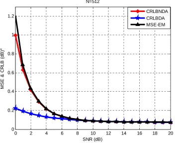
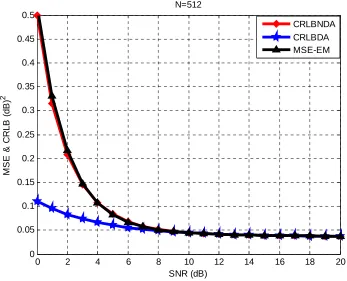
Figure 4.2 The MSE & CRLB in dB2 vs. SNR in dB when N=512 for the BPSK case
Figure 4.2 shows the relation between MSE and CRLB vs. SNR for N=512. What we realize here is that the MSE & CRLB are decreased compared with the case when N=128. CRLB itself decreased from 0.3 dB2 for high SNR when N was 128, to less than 0.1 dB2 for high SNR when N is 512. Figure
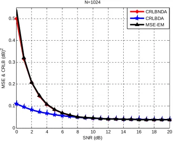
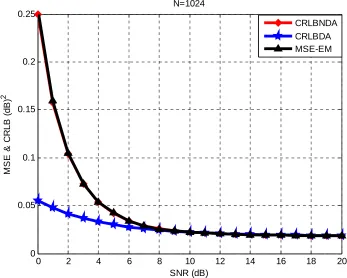
4.3 shows the same thing but for N=1024. Figure 4.3 shows that the precision of the MSE and CRLB is in the order of less than 0.05 dB2 for SNRs greater than 8 dB. Figure 4.4 shows the error which is
the difference between the MSE and CRLB in dB2 and the SNRs for the previous three cases of
different Ns, 128, 512, and 1024. This figure proves that as N increases, the error decreases which means that the MSE become closer and closer to the CRLB until they both match at some SNR value and beyond. From the SNR equation we see that the SNR is inversely proportional to the noise variance, which means as we increase the noise variance, the SNR will decrease as a result of that, and the two mixtures then will intervene with each other which makes it difficult for classification. On the other hand however, as we decrease the noise variance, the SNR will increase as a result of that and the two mixtures then will be far away from each other which makes classification become easier and results in almost no error..
0 2 4 6 8 10 12 14 16 18 20
0 0.2 0.4 0.6 0.8 1 1.2
SNR (dB)
M
SE & C
R
L
B
(
d
B)
2
N=512
Figure 4.3 The MSE & CRLB in dB2 vs. SNR in dB when N=1024 for the BPSK case
0 2 4 6 8 10 12 14 16 18 20
0 0.1 0.2 0.3 0.4 0.5
SNR (dB)
M
SE & C
R
L
B
(
d
B)
2
N=1024
CRLBNDA CRLBDA MSE-EM
0 2 4 6 8 10 12 14 16 18 20
0 0.5 1 1.5 2 2.5
SNR (dB)
E
rr
o
r i
n
(d
B
)
2
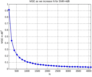
[image:48.612.132.466.423.682.2]Figure 4.5 The MSE in dB2 vs. N.
The last figure 4.5 which shows the changes in the MSE as we increase N. this is easily could be inferred from the previous figures, but we want it to be clear that as we increase N, MSE will decrease as a result. We vary N from 128 to 4096 and see the resultant MSE when SNR has been
chosen constant in this case to be 4 dB. The MSE decreased from 0.45 dB2 when N was 128 to about
0.025 dB2 when N is 4096. Our expectation is that as N tends to infinity, MSE will tend to zero as a
result
4.2TheQPSKcase
In the case of QPSK case, it is assumed that the received samples were drawn independently an identically from a mixture of four circular symmetric complex Gaussian distribution. Our model in this case would be exactly the same except for the transmitted symbols now four instead of two. We are assuming that there is no error in timing, phase deviation, or frequency deviation. The matched filter output may be given as,
, 1, … . . , 4.21
500 1000 1500 2000 2500 3000 3500 4000
0 0.1 0.2 0.3 0.4 0.5 0.6 0.7 0.8 0.9 1
N
MS
E
i
n
d
B
2
where, is the received sample, ∈
√ √ is the transmitted symbol, is the channel gain,
and is a zero mean AWGN with variance .
We can write equation (4.21) in a vector form as,
4.22
where, . . . . , . . . . , . . .. . The transmitted
symbols may be modeled as realizations of . . . circular symmetric complex Gaussian distribution. The probability distribution function may be written as,
/ , Ө 1 exp 1 | | 4.23
Assuming equally likely symbols,
; Ө / , Ө /Ө
1 1 4 1 1 √2 1 √2 1 4 1 1 √2 1 √2 1 4 1 1 √2 1 √2 1 4 1 1 √2 1 √2 1 1 4 1 √2 1 1 √2 1 1 √2 1 1 √2 1 | | ∗
; Ө 1 1 4
1
4
1
4
1
4
1
4
; Ө 1 1
4
| |
2
4 2
4
2
4 2
4
; Ө 1 1
4
| |
2 2
4
2 2
4
; Ө 1 1
2
| |
2
4 2
4
; Ө 1 | | √2 √2
The probability distribution function of N . . . received samples of will be as follows,
; Ө 1 | | √2 √2 4.24
The Log Likelihood function is then defined as follows,
Ө 1 | | √2 √2
1 | | √2 √2 4.25
This is the Log Likelihood function of the received data of , nowthe problem of estimation would
be as follows, given the observation vector, , estimate the parameters, Ө . Then use them
to find the SNR estimate,
10
4.2.1 TheCRLBforQPSK
The Cramer‐Rao Lower Bound (CRLB) is a lower bound for the Mean Square Error (MSE) of any unbiased estimator which satisfies the regularity condition [2]. In our case of SNR estimation, the CRLB can be given as,
Ө Ө Ө
Where Ө is the fisher information matrix given by,
Ө
; Ө ; Ө
; Ө ; Ө
And,
Ө
20 10
10
10
FortheNDAcase,
Ө 1 | | √2 √2
This procedure is similar to the one which being done by Alagha [8],
Ө
2 1 2 4
4
1 4
4.26
where,
2
√ 2 4.27
We can now substitute this result in equation (4.5) and get the following,
20 10
10 10
2 1 2 4
4
1 4
20 10 10
10
100 10
1 2 2
1 2 4 4.28
FortheDAcase,
The log likelihood function is given by,
Ө / , Ө
Ө 1 exp | |
| |
Ө 2
0
0
20 10
10 10
2 0
0
20 10 10
10
100 10
2
1 4.29
4.2.2 NDASNRestimationusingtheEMalgorithm
We use the EM algorithm now in estimating the SNR, its MSE and compare our estimated values with the CRLB values. Our assumptions are that the data was drawn from a mixture of four Gaussians, and are uncorrelated with each other. The samples are drawn in an . . . manner. The parameters which we need to estimate now are,
Ө
Ө
; Ө
10 4.30
The EM algorithm will be used to iteratively estimate the channel gain and the noise variance then use them to estimate the signal to noise ratio. The received data will be seen as incomplete data set since we don’t know the class of each transmitted symbol. The auxiliary function in this case may be given by,
Ө , Ө / , Ө / , Ө
/ , Ө
Ө , Ө / , Ө 1
2 ∑
/ , Ө 1
2 2 ∑
/ , Ө
/ ,
Ө
1Ө , Ө / , Ө
Ө
Ө
Ө , Ө
4.31
Now solving those two equations will give us the E & M steps.
When solving for the channel gain we get,
Ө , Ө
/ , Ө 0
Ө , Ө
/ , Ө 0
/ , Ө 2 2 ∗ 0
/ , Ө exp 2 1 /4
/ , Ө exp /4 / , Ө exp 3 /4
/ , Ө exp 5 /4 / , Ө exp 7 /4
/ , Ө 1 / , Ө / , Ө / , Ө
/ , Ө exp /4 / , Ө exp 3 /4
/ , Ө exp 5 /4
1 / , Ө / , Ө / , Ө exp 7 /4
/ , Ө exp /4 exp 7 /4
/ , Ө exp 3 /4 exp 7 /4
/ , Ө exp 5 /4 exp 7 /4 exp 7 /4
√2
/ , Ө / , Ө 1 / , Ө
1
2 1
√2
/ , Ө / , Ө 1
2
/ , Ө / , Ө 1
2 4.32
When solving for the variance we get,
Ө , Ө
/ , Ө 1 0
/ , Ө
/ , Ө / , Ө
/ , Ө
1 / , Ө / , Ө / , Ө
/ , Ө 2 ∗ 2 ∗
/ , Ө 2 ∗ 2 ∗
/ , Ө 2 ∗ 2 ∗
2 / , Ө exp /4 exp 7 /4
2 / , Ө exp 3 /4 exp 7 /4
2 / , Ө exp 5 /4 exp 7 /4
2 / , Ө √2 2 / , Ө 2 1
2 / , Ө √2
2√2
/ , Ө / , Ө 1
/ , Ө 1
2√2
/ , Ө / , Ө 1
2
/ , Ө / , Ө 1
2
1
2√2| |
1 2√2
1
| | 4.33
We don’t need to worry about the mixing coefficient since we know that they are equally likely. After Starting with initial values for the channel gain and noise variance, equations (4.27) and (4.28) will be used to iteratively find the estimates to the parameters which would be then used to
estimate the as given above. The will be found for different estimated values of different
[image:58.612.128.474.348.635.2]SNR values and will be assessed sing the CRLB.
Figure 4.6 The MSE & CRLB in dB2 vs. SNR in dB when N=128
0 2 4 6 8 10 12 14 16 18 20
0 0.5 1 1.5 2 2.5 3
SNR (dB)
M
SE & C
R
L
B (
d
B)
2
N=128
dB, and for different values of received sample size N, 128, 512, and 1024. Figure 4.6 shown explains three things when QPSK is used as the transmitted symbols. The red curve is the CRLB for NDA signal, the blue curve is the CRLB for DA signal, and the black curve which shows the MSE estimated using the EM algorithm. The EM algorithm SNR estimate is repeated 10000 times using Monte Carlo simulations to get 10000 realizations of the SNR estimates, then averaging them to get the estimated SNR, and find their variance to get the MSE for that specific SNR estimate value.
Figure 4.7 The MSE & CRLB in dB2 vs. SNR in dB when N=512
We then repeat this process for different values of SNR, say from 0 dB to 20 dB and their resultant MSE. Those estimates then compared with the CRLB as shown above. We see that for low SNR estimate values; the MSE is large compared with the NDA CRLB. The higher the SNR become, the lower the MSE we get till they (the CRLB and MSE) both match. This was for sample size of N=128 in figure 4.6 in the previous page. The next step we would do is increase N and see what is going to happen to our estimation accuracy. Figure 4.7 shows the relation between MSE and CRLB vs. SNR for N=512. What we realize here is that the MSE is decreased, also CRLB is decreased from what it was before when N=128. CRLB itself decreased from 2 when N was 128 and SNR of 0dB, to less than 0.5 when N is 512 at the same SNR.
0 2 4 6 8 10 12 14 16 18 20
0 0.05 0.1 0.15 0.2 0.25 0.3 0.35 0.4 0.45 0.5
SNR (dB)
M
SE &
C
R
L
B (
d
B
)
2
N=512
Figure 4.8. The MSE & CRLB in dB2 vs. SNR in dB when N=1024
0 2 4 6 8 10 12 14 16 18 20
0 0.05 0.1 0.15 0.2 0.25
SNR (dB)
M
SE & C
R
L
B (
d
B)
2
N=1024
CRLBNDA CRLBDA MSE-EM
0 2 4 6 8 10 12 14 16 18 20
0 0.5 1 1.5
E
rror i
n
(dB
)
2
[image:60.612.133.467.422.689.2]Figure 4.8 shows the same thing Figure 4.7 shows, but for N=1024. The precision of the MSE and CRLB is in the order of less than 0.025 dB2 for SNRs greater than 6 dB. Figure 4.9 shows the error
which is the difference between the MSE and NDA CRLB in dB2 at different values of SNRs shown
5. MISOwithSTBCNDASNRestimationusingtheExpectationMaximizationalgorithm
Modern communication systems require accurate estimation of the Signal to Noise Ratio SNR for optimal usage of radio resources [5], [9]. The knowledge of the SNR is a requirement in most applications in order to make optimal signal detection, power control. MIMO systems gives a significant enhancement to the accuracy of estimating the SNR besides many other improvements in data rate, channel capacity, and being able to reduce Multipath fading at the remote units. Different diversity modes are being used, time diversity, frequency diversity, spatial diversity. A MIMO system usually consists of M transmit and N receive antennas. Attention will be given to the transmit diversity for some reasons, which then will be compared with SISO and SIMO. Transmit diversity or MISO would improve our system’s performance without the cost, size, and power that SIMO will have in order to improve the quality of the received signal [12]. For that reason, antenna diversity techniques are utilized at the Base station. A simple transmit diversity technique will be explained here which been done by Alamouti in [12]. Space‐time codes are used to generate a redundant signal. The signal copy is transmitted not only from a different antenna, but at a different time. The signal s1 and s2 are sent in the first symbol, then a signal
replication of –s2* and s1* is added to create the Alamouti space‐time block code. 5.1ConventionalReceivediversity(SIMO)model:
h
h2
hNR
TX#1
RX#1
RX#2
Combining
sch
em
e
[image:62.612.110.511.443.701.2]h1
h2
hNT
where i=1, 2, . . . , NR. and n=1, 2, . . . , N.
/ , Ө 1 exp
/ , Ө 1 exp
5.2Transmitdiversity(MISO)model:
[image:63.612.111.473.268.709.2]
Figure 5.2 MISO/ Transmit diversity system model
where i=1, 2, . . . , NT. and n=1, 2, . . . , N.
/ , Ө 1 exp ∑ 1
/ , Ө 1 exp ∑ 1
TX#1
TX#2
TX#N
5.3MIMOmodel:
Figure 5.3 MIMO system model
where i=1, 2, . . . , NT, j=1, 2, . . . , NR , and n=1, 2, . . . , N, and hij is the channel gain
between the transmit antenna i and the receive antenna j.
/ , Ө 1 exp
/ , Ө 1 exp
TX#1
TX#2
TX#N
RX#1
RX#2
RX#NR
h11
5.4ThetransmitdiversityforBPSKcase:
This approach is being done by Alamouti [12] where two transmit antennas and one receive antenna has been used. At a given time, n, two signals are simultaneously sent from the two antennas. Denoting the signal sent by antenna one by, S1, and the signal sent by antenna two
by, S2. Then we repeat sending – S2* from the first antenna, then S1* from the second
antenna, this ordering will be done to all of our data. This is called space and time coding. Our model in this case will look like,
∗ ∗
We then may write it in a matrix form as,
∗ ∗ ∗ , 1,2, … . . , /2. 5.1
⊗
where R(n) is the received samples from both antennas at time n, H is the complex channels gains matrix, S(n) are the sent symbols at time n from the two antennas, W(n) are the Circularly symmetric complex Gaussian noise samples at time n, R is the vector of received
samples, I is Identity matrix where N is the total number of received samples, S is the
sent vector of symbols, W is the noise vector at the receiver, ⊗ is the kroncker product, and H is as follows;
∗ ∗
The probability distribution function for the received data at a given time n, given the transmitted data, given by,
/ , Ө 1 exp ‖ ‖ 5.2
; Ө / , Ө /Ө
Suppose an equally likely data symbols.
; Ө 1
4 exp
‖ ‖
; Ө 1
4 exp
| | | |
For the BPSK case, 1, 1 , 1, 1 .
where ∈ 1
1 , 1
1 , 11 , 1 1 .
We can then rewrite ; Ө as follows,
; Ө 1
4 exp
| | | |
exp | | | |
exp | | | |
exp | | | |
; Ө 1
4 exp
| | | | 2 ∗ 2 ∗ | | | |
exp | | | | 2 ∗ 2 ∗ | | | |
exp | | | | 2
∗ 2 ∗ | | | |
exp | | | | 2 ∗ 2 ∗ | | | |
; Ө 1
4 exp
| | | | | | | |
exp 2 ∗ 2
∗
exp 2 ∗ 2 ∗
exp 2 ∗ 2
∗
exp 2
∗ 2 ∗
; Ө 1
4 exp
| | | | | | | |
∗ 2 cosh 2 ∗ 2 ∗
2cosh 2 ∗ 2 ∗
We know that,
cosh cosh 2cosh
2 cosh 2
; Ө 1
2 exp
| | | | | | | |
∗ 2 cosh 2
∗ 2 ∗
cosh 2
∗ 2 ∗
; Ө 1 exp | | | | 2| | 2| |
∗ cosh 2
∗ 2 ∗
cosh 2
∗ 2 ∗
5.3
For N . . . received samples of R(n), the Joint PDF distribution will be written as follows,
; Ө 1 exp | | | | 2| | 2| |
/
∗ cosh 2
∗ 2 ∗
cosh 2
∗ 2 ∗
5.4
Ө ; Ө
/
Ө 1 exp | | | | 2| | 2| |
/
∗ cosh 2
∗ 2 ∗
cosh 2
∗ 2 ∗
Ө
/
| | | | 2| | 2| |
cosh 2
∗ 2 ∗
cosh 2
∗ 2 ∗
5.5
Now given the received sample R, estimate the parameters h1, h2, and . However, h1, h2 are
complex variables, so we need to estimate their real and imaginary parts separately.
Let
Now our parameters are as follows,
Ө ̂
Ө
; Ө
5.5TheCRLBforthetransmitdiversityintheBPSKcase.
FortheDAcase:
In this case we are assuming that we know the transmitted data S and would like to find a lower
bound on the variance in this case. We know that CRLB is given by,
Ө Ө Ө
where Ө is the fisher information matrix given by,
Ө ; Ө
Ө Ө
And,
Ө
20 10
20 10
20 10
20 10
10 10
where | | | | .
/ , Ө 1 exp ‖ ‖
/ , Ө 1 exp ‖ ‖
/
Ө
/
‖ ‖
/
| | | |
/
/
| | | ∗ |
/
∗ ∗
Ө / 1
2 2 ∗
Ө / 1
2 2
1
/
2 2
1
Ө / 1
4 2
Ө Ө Ө Ө Ө Ө Ө
Ө 2
, Ө Ө
Ө Ө
Ө Ө
2
0 0 0 0
0 2 0 0 0
0 0 2 0 0
0 0 0 2 0
0 0 0 0 1
Ө Ө Ө
20 10 20 10 20 10 20 10 10 10 2
0 0 0 0
0 2 0 0 0
0 0 2 0 0
0 0 0 2 0
0 0 0 0
20 10 20 10 20 10 20 10 10 10 100 log 10 2
1 5.7
FortheNDAcase:
Ө
/
| | | | 2| | 2| |
cosh 2
∗ 2 ∗
cosh 2
∗ 2 ∗
We need to find the fisher information matrix for this Likelihood function in order to find the CRLB for the NDA case.
Ө Ө
Ө Ө , Ө Ө , Ө Ө ,
Ө Ө , Ө Ө , Ө Ө ,
Ө Ө , Ө Ө , Ө Ө ,
Ө Ө , Ө Ө , Ө Ө
Ө Ө , Ө Ө , Ө Ө .
Ө / 4 2 ∗ 2 ∗ 2 ∗
2 ∗ 2 ∗ 2
Ө / 2 ∗ 2 ∗ 2 ∗ 2 ∗
2 ∗ 2 ∗ 2 2
Ө / 2 ∗ 2 ∗ 2 ∗ 2
2 ∗ 2 ∗ 2 2 ∗
Ө / 2 ∗ 2 ∗ 2 ∗ 2
Ө / 4 2 ∗ 2 ∗ 2 ∗
2 ∗ 2 ∗ 2 ∗ 2 ∗ 2 ∗
2 ∗ 2 ∗ 2
2 ∗ 2 ∗ 2 2 ∗ 2 ∗
Ө / 4 2 ∗ 2 ∗ 2 ∗
2 ∗ 2 ∗ 2
Ө / 2 ∗ 2 ∗ 2 ∗ 2
2 ∗ 2 ∗ 2 2 ∗
Ө / 2 ∗ 2 ∗ 2 ∗ 2
2 ∗ 2 ∗ 2 2 ∗
Ө / 4 2 ∗ 2 ∗ 2 ∗
2 ∗ 2 ∗ 2 ∗ 2 ∗ 2 ∗
2 ∗ 2 ∗ 2
Ө / 4 2 ∗ 2 ∗ 2
2 ∗ 2 ∗ 2 ∗
Ө / 2 ∗ 2 ∗ 2 2
2 ∗ 2 ∗ 2 ∗ 2 ∗
Ө / 4 2 ∗ 2 ∗ 2
2 ∗ 2 ∗ 2 2 ∗ 2 ∗
2 ∗ 2 ∗ 2 ∗
2 ∗ 2 ∗ 2 ∗ 2 ∗ 2 ∗
Ө / 4 2 ∗ 2 ∗ 2
2 ∗ 2 ∗ 2 ∗
Ө / 4 2 ∗ 2 ∗ 2
2 ∗ 2 ∗ 2 2 ∗ 2 ∗
2 ∗ 2 ∗ 2 ∗