An EM algorithm for maximum likelihood estimation of process factor analysis models

(1)

AN EM ALGORITHM FOR MAXIMUM LIKELIHOOD

ESTIMATION OF PROCESS FACTOR ANALYSIS MODELS

Taehun Lee

A dissertation submitted to the faculty of the University of North Carolina at Chapel Hill in partial fulfillment of the requirements for the degree of Doctor of Philosophy in the Department of Psychology (Quantitative).

Chapel Hill 2010

Approved by

Robert C. MacCallum, Ph.D.

Stephen H. C. du Toit, Ph.D.

David M. Thissen, Ph.D.

Kenneth A. Bollen, Ph.D.

(2)

c 2010 Taehun Lee

(3)

ABSTRACT

Taehun Lee: AN EM ALGORITHM FOR MAXIMUM LIKELIHOOD ESTIMATION OF PROCESS FACTOR ANALYSIS MODELS

(Under the direction of Robert C. MacCallum and Stephen H. C. du Toit)

In this dissertation, an Expectation-Maximization (EM) algorithm is developed and im-plemented to obtain maximum likelihood estimates of the parameters and the associated standard error estimates characterizing temporal flows for the latent variable time se-ries following stationary vector ARMA processes, as well as the parameters defining the relationship between the latent stochastic vector and the observed scores taking mea-surement errors into account. Such models have been known as Process Factor Analysis (PFA) models (Browne & Nesselroade, 2005). In theE-step, the complete-data expected log-likelihood, the so-calledQ-function, which is the joint likelihood of the manifest vari-ables and the latent time series process varivari-ables, is constructed by supposing the latent process variables are observed. In the M-step, the Newton-Raphson algorithm is em-ployed in order to update the parameter estimates. The closed form expressions for the gradient vector and the Hessian matrix of the target function are derived for implement-ing the M-step of the EM algorithm. Methods for obtaining the associated standard error estimates are developed and implemented. The proposed EM algorithm employs the covariance structure derived by du Toit and Browne (2007) where the influence of the time series prior to the first observation has remained stable and unchanged when the first observations are made. Thus, unlike other conventional structural equation modeling (SEM) software, model implied covariance matrices satisfy the stability condition and are Block-Toeplitz matrices. The proposed algorithm is applied to simulated data in order to

(4)

(5)

ACKNOWLEDGEMENTS

First and foremost, I am especially grateful to my mentor, Dr. Robert, C. MacCal-lum, whose encouragement, supervision and support enabled me to successfully complete five years of graduate careers in L. L. Thurstone Psychometric Laboratory. I wish to ac-knowledge all of my committee members for their insightful feedback on my dissertation. It would have been impossible to write this dissertation without your help and guidance. I especially wish to thank Dr. Stephen, H. C. du Toit, whose encouragement and guidance from the preliminary to the concluding level enabled me to develop an under-standing of the subject. I am indebted to him who supported the project with a grant from NIAAA, SBIR Phase 2 grant (5R44AA014999-03).

I am thankful to Dr. Cheongtag Kim, who introduced me to the field of Psycho-metrics. I have vivid memories of the exciting moments when I first encountered this dynamic, challenging, and exciting field. I also wish to thank student colleagues of L. L. Thurstone Psychometric Laboratory for their intellectual challenge, support, and friend-ship.

Lastly, I am heartily thankful to my wife, always being there for me. You are a wonderful wife to me and a wonderful mother to our son, Sean Lee.

(6)

To my parents, Sanghwan Lee and Sunjin Sohn,

To my son, Sean Lee,

And

(7)

CHAPTER

1 Introduction . . . 1

2 Objectives . . . 5

3 Method of maximum likelihood and the EM algorithm . . . 7

3.1 The EM algorithm as a method to obtain MLE . . . 9

3.2 The monotonicity of the EM algorithm . . . 11

4 Introduction to Process Factor Analysis . . . 12

4.1 The model specification . . . 13

4.2 Relationships to other dynamic factor analysis models . . . 15

4.3 The covariance structure of the latent stationary VARMA(p, q) model . 16 5 Maximum likelihood estimation for the PFA model by the EM algo-rithm . . . 20

5.1 The general expression . . . 20

5.2 The conditional likelihood function ofY given η . . . 21

5.3 The marginal likelihood function of η . . . 23

5.4 The complete-data log-likelihood ofY and η . . . 23

5.5 The analytic gradient vector and Hessian matrix of Q-function . . . 24

6 Estimation of Standard Errors for Parameter Estimates . . . 37

6.1 The principle of missing information . . . 37

(8)

6.2 Previous studies on standard error estimation . . . 38

6.3 The derivation of the missing information matrix . . . 40

7 A study of parameter recovery of the proposed EM Algorithm . . . 43

7.1 The first case: repeated time-series withN = 500 and T = 5 . . . 44

7.2 The second case: repeated time-series withN = 10 and T = 50 . . . 48

7.3 The third case: single-subject time series withN = 1 and T = 100 . . . 49

8 Discussion . . . 62

8.1 Objectives accomplished . . . 62

8.2 A methodological implication of the objectives accomplished . . . 63

8.3 A substantive implication of the objectives accomplished . . . 64

8.4 On the analysis of non-stationary data under the proposed algorithm . . 64

8.5 On relationships to the quasi-simplex model . . . 65

8.6 Future studies . . . 67

8.6.1 Starting values . . . 67

8.6.2 Comprehensive measurement models . . . 68

8.6.3 Identification of order of latent time series . . . 69

8.7 Conclusion . . . 70

APPENDICES

A Proof of equations (5.9) and (5.10) . . . 71

B The closed form expressions for typical elements of missing information matrix . . . 73

(9)

LIST OF TABLES

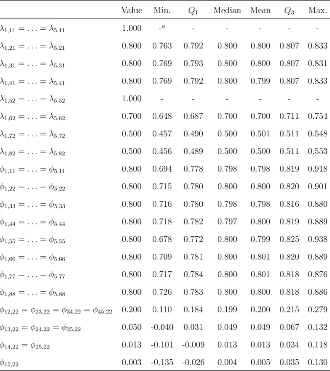
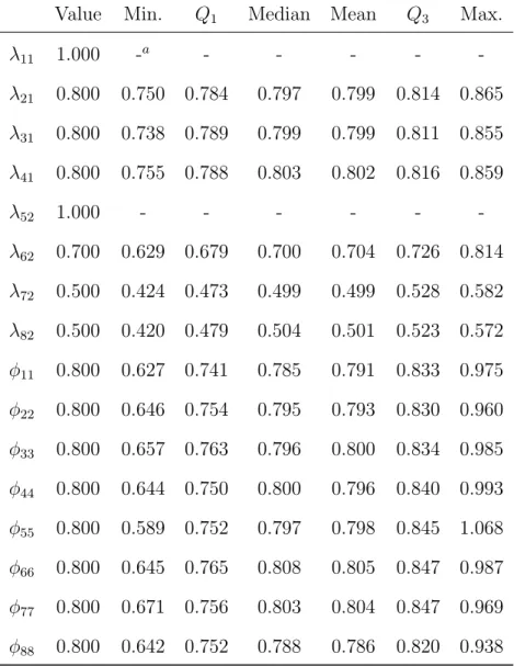
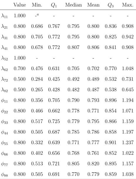
7.1 Summary of the maximum likelihood estimates of free parameters in Λ and Φ obtained from the simulation study (1,000 replications, T=5,N=500 PFA(1,1)). 50

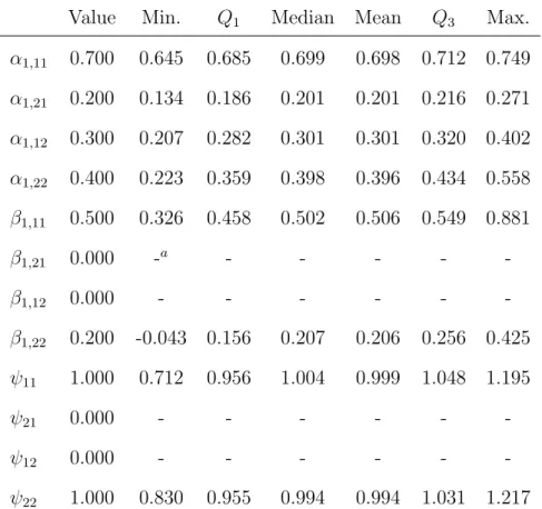
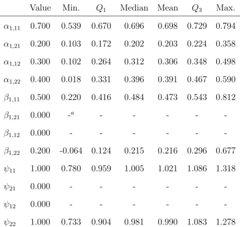
7.2 Summary of the maximum likelihood estimates of free parameters in A1, B1,

and Ψ obtained from the simulation study (1,000 replications, T=5, N=500, PFA(1,1)). . . 51

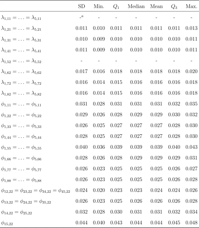
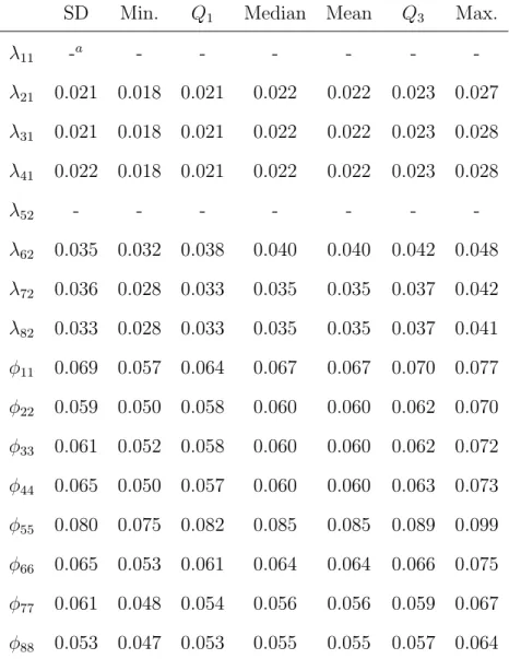
7.3 Summary of the standard error estimates associated with free parameters in Λ and Φ obtained from the simulation study (1,000 replications, T=5, N=500, PFA(1,1)). . . 52

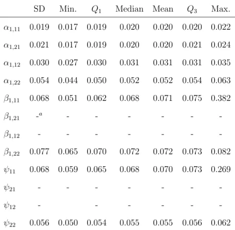
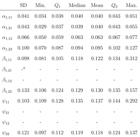
7.4 Summary of the standard error estimates associated with free parameters in

A1, B1, and Ψ obtained from the simulation study (1,000 replications, T=5,

N=500, PFA(1,1)). . . 53

7.5 Summary of the maximum likelihood estimates of free parameters in Λ and Φ obtained from the simulation study (1,000 replications, T=50, N=10, PFA(1,1)). 54

7.8 Summary of the standard error estimates associated with free parameters in

A1,B1, and Ψ obtained from the simulation study (1,000 replications, T=50,

N=10, PFA(1,1)). . . 57

7.9 Summary of the maximum likelihood estimates of free parameters in Λ and Φ obtained from the simulation study (1,000 replications, T=100, N=1, PFA(1,1)). 58

(10)

7.12 Summary of the standard error estimates associated with free parameters in A1,B1, and Ψ obtained from the simulation study (1,000 replications, T=100,

(11)

LIST OF FIGURES

4.1 VARMA(1,1) Time Series, m = 2, T = 5 . . . 14

(12)

Chapter 1

Introduction

In psychological research, it is common for researchers to administer a battery of measures that allow inferences about unobserved latent factors that are presumed to underlie the observed measures. In cross-sectional data analysis, when the central theme of research is to investigate correlational or causal relationships among latent factors, latent variable modeling such as factor analysis, structural equation modeling (SEM), and item response theory (IRT) have been routinely employed and commercial software is readily available to applied researchers.

However, when the central theme of research is to investigate psychological processes of latent factors, (e.g. whether conscientiousness shows any dramatic change over time, how the change in conscientiousness is related to the change in emotional stability, etc.) a new development dealing with a sequence of measurements taking measurement error into account is necessary in terms of model specification and parameter estimation.

(13)

by J¨oreskog (1970) to fit a nonstationary first order autoregressive (AR) process model, known as the Simplex model, SEM methodology has been used frequently for modeling time series data in psychology (Browne & Zhang, 2007b).

For example, in the context of a univariate time series observed in a single sub-ject, van Buuren (1997) investigated how the stationary autoregressive moving average (ARMA) model can be formulated and fitted as a structural equation model using a lagged covariance matrix. In a slightly different context where the number of measure-ments T is intermediate, say, T = 30 and the sample size is small, say, N = 5, Hamaker, Dolan, and Molenaar (2003) showed how the raw data maximum likelihood method, which is conventionally adopted for modeling incomplete data in SEM software, can be effectively employed to estimate autoregressive and moving average coefficients in a univariate ARMA model. Recently, du Toit and Browne (2007) developed the model specification for the covariance structure of a vector ARMA time series compatible with conventional SEM software. The derived expression is suitable both for the covariance structure of a single-subject time series and for the covariance structure of a repeated time series in a random sample of subjects.

The idea for fitting a (vector) ARMA model in SEM software is as follows. In a repeated time series, where a sequence of observations on k variables at T time points for each of n = 1, . . . , N subjects, which amounts to N ×T ×k observations in all, are obtained and assumed to follow the same vector ARMA (VARMA) process, the usual sample covariance matrix, S can be calculated and a structural equation modeling program such as LISREL may be used to fit a VARMA covariance structure.

In other situations, where a single time series, a sequence of observations on multiple variables on a single subject at regular intervals over time, is being analyzed, there are two alternative approaches that may be used (du Toit & Browne, 2007). One is to calculate autocovariance matrices and analyze them using structural equation modeling software (Hamaker, Dolan, & Molenaar, 2002; Nesselroade, McArdle, Aggen, & Meyers, 2002; van

(14)

Buuren, 1997). The other alternative is to maximize the log-likelihood function based on a single set of repeated measurements. Some structural equation modeling programs providing full information maximum likelihood estimates by considering subjects one at a time can be adapted to estimating a single subject times series model. An alternative is to use the Kalman filter in conjunction with the prediction error decomposition of the log-likelihood function of an ARMA model (Engle & Watson, 1981), but this approach can not be implemented with available SEM software.

An advantage of the aforementioned approaches is that some of them can be readily implemented with available SEM software. Those available SEM programs, however, do not provide facilities for imposing complicated stability constraints on the autoregressive weight matrices and inequality constraints on the moving average weight matrices for identification (Brockwell & Davis, 2002; du Toit & Browne, 2007). More importantly, none of the available SEM software can accommodate the specification of the covariance structure of a VARMA(p, q) times series model with the stationarity condition imposed (du Toit & Browne, 2007) although, in the case of a VARMA(1,1), this might be accom-plished in LISREL by imposing complicated constraints on the time series parameters1_.

In other words, when the psychological process has started in the distant past and the parameters have remained constant throughout so that the stability conditions are sat-isfied, there is no way of implementing this constraint in estimating parameters using available SEM software. In particular, although the autocorrelation approach must as-sume that a sample of observations is generated by a stationary underlying process, conventional SEM software does not provide an easy way of constructing appropriate model-implied covariance structure matrices of Block-Toepliz form with the stationariy condition imposed.

The autocorrelation approach has an additional danger because the independence assumption required for the autocovariance matrices to follow the Wishart distribution

(15)

is routinely violated. Consequently standard error estimates and test statistics produced by these programs have no theoretical foundation. A least squares estimation method combined with bootstrapping has been proposed (Zhang, 2006) based on the autocorre-lation matrix but the resultant estimates do not have the desirable statistical properties of maximum likelihood estimates.

Above all, the current approaches are restricted to modeling univariate time series data of manifest variables disregarding measurement error, which plays a crucial role in psychometric methodology such as factor analysis and latent variable modeling in psychological research. In other words, when the observed scores at time t, say, yt may

be decomposed into the three components of a deterministic trend (µt), a latent stochastic

component (ft), and a measurement error (εt), and one desires to model the dynamic

processes of the latent component (ft) using a VARMA time series, new developments are

necessary in terms of model specifications and parameter estimations. Furthermore, when dynamic processes are assumed to be stationary, to the best of the author’s knowledge, no existing SEM software possesses the facility of estimating AR and MA coefficients for the latent variable VARMA models with the nonlinear constraints of the stationarity condition imposed. In addition, as Hamaker et al. (2003) pointed out, the parameter estimates obtained from SEM software based on autocovariance matrix are not true maximum likelihood estimates.

(16)

Chapter 2

Objectives

The goal of this dissertation is to develop and implement an Expectation-Maximization (EM) algorithm to obtain maximum likelihood estimates (MLEs) of the AR and MA coefficients characterizing the latent time series following stationary VARMA processes as well as the parameters defining the relationship between the latent stochas-tic vector and the observed scores taking measurement errors into account. Such models have been known as Process Factor Analysis (PFA) models in psychological research (Browne & Nesselroade, 2005). The closed form expressions of the gradient vector and the Hessian matrix for implementing the M-step of the EM algorithm will be derived in such a way that they can be readily implemented in SEM software such as LISREL (J¨oreskog & S¨orbom, 2006).

In order to ascertain that the proposed EM algorithm and the associated gradient vector and Hessian matrix are suitable to maximize the expected complete data log-likelihood to obtain the MLEs, a simulation study will be conducted with known values of parameters. The proposed algorithm will be implemented in the general scientific com-puting program, R (R Development Core Team, 2009) and resulting parameter estimates will be compared to the specified population parameter values.

(17)

this criticism, either. In this dissertation project, a method for standard error estimation is developed and its performance is evaluated by comparing the estimates and the actual variability of the parameter estimates obtained in the simulation study.

The remainder of this dissertation is organized as follows. First, after a brief review of maximum likelihood estimation and the EM algorithm, the PFA model is introduced with the associated covariance structure originally derived by du Toit and Browne (2007) briefly reproduced. Next, the E-step and the M-step are described to implement the EM algorithm for obtaining maximum likelihood estimates for PFA models. Details of derivation of the gradient vector and the Hessian matrix are described. Then, a method for standard error estimation is developed. The performances of the proposed EM algorithm and standard error estimation method are then investigated by application to simulated data. Finally, relevant methodological issues and future research plans are discussed.

(18)

Chapter 3

Method of maximum likelihood and the EM algorithm

Suppose that random vector, Y has the density function f(Y|γ), where Y = (Y1, . . . , Yn)0 and γ = (γ1, . . . , γq)0. Given the observed data y = (y1, . . . , yn)0 and a

statistical model parameterized by a q×1 unknown vector of values, γ, the likelihood function L(γ|y) is any function of γ proportional to f(y|γ). The likelihood function provides us with a measure of relative preferences for various parameter values and the maximum likelihood estimate (MLE), denoted by ˆγ, provides a point estimate for a vector of parameters of interest that makes the observed data most likely.

Under certain regularity conditions, maximum likelihood estimators possess so-called asymptotically optimal properties (Bickel & Doksum, 2001; van der Vaart, 1998; Lehmann & Casella, 1998). That is, as sample size approaches infinity, the bias of MLE tends to zero (asymptotically unbiased), and the variance of the MLE tends to the inverse Fisher information, achieveing the Cram´er-Rao lower bound (asymptotic efficiency). In addition, as the sample size tends to infinity, the distribution of MLE converges to the normal distribution with mean equal to the true value of the parameter and covariance matrix equal to the inverse of the Fisher-information matrix . This is practically a very important result because we may treat ˆγ as a normal variate with mean γ and with covariance that can be calculated from a knowledge of the postulated density f(Y|γ).

(19)

the value of γ that maximizes the log-likelihood function, `(γ|y). If `(γ|y) has partial derivatives with respect to γ1, . . . , γq, then ˆγ can be obtained by solving the likelihood

equations,

∂`(γ|y) ∂γr

= 0, r= 1, . . . , q (3.1)

In general situations, one may use an iterative numerical method to locate a mode of the likelihood function,i.e. MLE. Letγ(0) _{denote an initial guess of ˆ}_γ _{and let}_γ(i) _denote

the guess at theıth _{iteration. Then, one such algorithm, the Newton-Raphson algorithm,}

is given as

γ(ı+1) =γ(ı)+

−∂

2_`(γ|Y₎

∂γ ∂γ0

−1

γ=γ(ı)

_∂`(γ|Y

) ∂γ

γ=γ(ı)

(3.2) The vector of first-order partial derivatives of a function is called the gradient vector and the symmetric matrix of second-order partial derivatives of a function is called the Hessian matrix. In the present setting, the gradient vector and the Hessian matrix are given as ∂`(_∂γγ|Y) and ∂_{∂γ ∂γ}2`(γ|Y0), respectively. If the log-likelihood function is quadratic, this

algorithm converges in one iteration from any starting value. For general functions, this method gives quadratic convergence near the minimum. As can be seen in equation (3.2), the Newton-Raphson algorithm requires the gradient vector and the Hessian matrix of the log-likelihood function, which may not be a trivial task in highly parameterized models. However, when converged, this algorithm provides the asymptotic variance-covariance matrix associated with the parameter estimates as its natural by-product. The expec-tation of the negative Hessian matrix is called the Fisher information matrix and the asymptotic variance-covariance matrix is given by the inverse of the Fisher information matrix evaluated at MLEi.e. −Eh∂_{∂γ ∂γ}2`(γ|Y0)

i−1

γ=ˆγ . The Fisher-Scoring algorithm, an

alter-native approach to the Newton-Raphson algorithm, replaces the Hessian matrix by its expectation, which is given by

γ(ı+1) =γ(ı)+

−E

∂2`(γ|Y) ∂γ ∂γ0

−1

γ=γ(ı)

∂`(γ|Y) ∂γ

γ=γ(ı)

(3.3)

(20)

The Newton-Raphson and Fisher-Scoring algorithms have been important tools for finding MLE in the context of factor analysis and structural equation modeling (J¨oreskog, 1966, 1967, 1969, 1971; Bock & Bargmann, 1966; du Toit & du Toit, 2008).

3.1 The EM algorithm as a method to obtain MLE

The Newton-Raphson algorithm is a calculus-based method that can be employed for finding the zeroes (or roots) of a real-valued function in general. On the other hand, the EM algorithm is a statistically motivated algorithm where missing data are involved and the analysis of the likelihood function based on the observed data is somewhat complicated. The notion of ‘missingness’ does not have to involve actual missing data but any incomplete information. For example, unobservable latent variables can be treated as missing (Dempster, Laird, & Rubin, 1977).

The EM algorithm is a type of data augmentation algorithm in which one augments the observed dataY with the unobservedmissing orlatent data Z. The augmented data X = (Y, Z) are called thecomplete data, whilep(X|γ), the associated likelihood function of X, is termed the complete data likelihood function. Specifically, while the observed data likelihood function p(Y|γ) is difficult to maximize with respect to γ, the augmented or the complete data likelihood function p(Y, Z|γ) is simple to maximize with respect to γ. The EM algorithm makes use of this simplicity in maximizing the observed data likelihood function (Schafer, 1997).

(21)

The EM algorithm consists of two steps called the expectation step (E-step) and the maximization step (M-step). In the E-step, the conditional expectations of the missing data are computed given the observed data and the current estimates of the parameters. These expected values are then substituted for the missing data and used to complete the data. In the M-step, maximum likelihood estimation of the parameters is performed in the usual manner using the completed data. The estimated parameters are then used to reestimate the missing data, which in turn lead to new parameter estimates. These two steps define an iterative procedure, which is repeated until convergence is achieved. Formally stated, the EM algorithm starts with an initial guess of the parameters, γ(0) _{and alternates the following two steps at} _`_{= 0,}_1,_{2, . . .: The}_E_{-step and the}_M_-step.

In the most general setting, theE-step computes the target function

Q(γ|γ(`)_{) =}

Z

lnp(Y, Z|γ)p(Z|γ(`)_{, Y}_{) dZ} _(3.4)

i.e. the expectation of lnp(Y, Z|γ) with respect to p(Z|γ(`)_{, Y}_{). In the} _M_{-step, the} _Q

function is maximized with respect to γ to obtainγ(`+1)_{. The algorithm is iterated until}

kγ(`+1)₋_γ(`)_k _or_|Q(γ(`+1)_|γ(`)₎₋_Q(γ(`)_|γ(`)_)| _{is sufficiently small.}

(22)

3.2 The monotonicity of the EM algorithm

One of the most important properties of the EM algorithm, known as monotonicity, is that it always increases the observed likelihood:

p(Y|γ(`+1)₎_≥_p(Y_|γ(`)₎ _(3.5)

The monotonicity of the EM algorithm in (3.5) can be shown as follows. Notice that p(Y, Z|γ) =p(Y|γ)p(Z|, Y γ), which implies

−lnp(Y|γ) = −lnp(Y, Z|γ) + lnp(Z|Y, γ) (3.6)

By taking the conditional expectation of (3.6) with respect to the density p(Z|Y, γ(`)₎

yields

h(γ|γ(`)_{) =} _Q(γ|γ(`)₎₋_ln_p(Y_|γ) _(3.7)

where h(γ|γ(`)_{) =} R

lnp(Z|Y, γ)p(Z|Y, γ(`)_{) dZ. Then, by the Kullback-Leibler}

informa-tion inequality, it can be shown that

h(γ|γ(`))≤h(γ(`)|γ(`)) (3.8)

Substituting (3.7) into (3.8) and rearranging the terms, we have

lnp(Y|γ(`+1)₎₋_ln_p(Y_|γ(`)₎_≥_Q(γ(`+1)_|γ(`)₎₋_Q(γ(`)_|γ(`)₎_≥₀ _(3.9)

By definition of γ(`+1) _{as the maximizer of} _Q(γ|γ(`)_{), the last inequality of (3.9) holds.}

(23)

Chapter 4

Introduction to Process Factor Analysis

The process factor analysis (PFA) model is a type of dynamic factor model. There are various definitions of a dynamic process but one that is adopted in this dissertation is “any natural process in which each succeeding state is a function of the preceding states plus a non-forecastable change” (Browne & Zhang, 2007b). Dynamic factor analysis models include variables representing the forces that cause change (random-shock variables), variables on which the change (outcomes) is actually manifested (process variables), and parameters that define, at least to some extent, a temporal flow in the relationships among and between the two kinds of variables (autoregressive and moving average coefficients) (Browne & Nesselroade, 2005). The random variable providing the dynamic force that changes the process variable is the so-called “white noise” variable or “random shock” variable. The values of random shock are unpredictable and produce sudden changes in the process variables (Browne & Nesselroade, 2005).

(24)

4.1 The model specification

In PFA models, the manifest variables, Yt are assumed to satisfy a factor analysis

model

Y_t=µ_t+λtηt+εt, t = 1, . . . , T (4.1)

where Yt represents a k×1 random vector of manifest variables at time t, µt is a k×1

mean vector, which can be constant, µt =µor may vary systematically with time, ηt is

an m×1 random vector representing latent common factors at time t, λt is a constant

k × m factor loading matrix at time t and εt is a k ×1 random vector representing

unique factors at time t. Unique factors are assumed to be independent of ηt for all t.

Common factors, ηt are regarded as process variables and they are assumed to follow a

VARMA(p, q) process, vector autoregressive of order p and moving average of order q process of the form:

η_t =A₁η_t₋₁+A₂η_t₋₂+· · ·+A_pη_t₋_p+z_t+B₁z_t₋₁ +B₂z_t₋₂+· · ·+B_qz_t₋_q (4.2)

where E(zt) = 0 and cov(zt, zt0) = Ψ. The elements of zt are mrandom shocks that drive

change in the m common factors.

The PFA model is given by Equation (4.1) and (4.2). In particular, (4.1) shows that the principal role of the observed variables is that of the indicator variables for the common factors of the form represented by Equation (4.2), which is one of major differences from previous attempts to specify and fit (vector) ARMA models where the process variables were manifest variables rather than latent variables.

Figure 4.1 shows a path diagram for a vector of two common factors following a stationary VARMA(1,1) time series, which can be given in the following scalar form equations:

η1,t =α11η1,t−1+α12η2,t−1+z1,t+β11z1,t−1

(25)

Figure 4.1: VARMA(1,1) Time Series, m= 2, T = 5

11

ψ ψ11 ψ ψ ψ

ψ

1,1

z z_1,2 z_1,3 z_1,4 z_1,5 1,0

z

11

ψ ψ11 ψ11 ψ11 ψ11

11

ψ

1 1 1 1 1

1

1 1

η η_{1 2} η1 3 η1 4 η1 5 1 0

η

11

β β11 β11 β11

11

β β11

1,1

η η_1,2 η1,3 η1,4 η1,5 1,0 η 11 α α 21 α 11 α α 21 α 11 α α 21 α 11 α α 21 α 11 α α 21 α 12

ψ ψ12 ψ12 ψ12 ψ12 ψ12

11 α α 21 α 2,1

η η_2,2 η_2,3 η_2,4 η_2,5

2,0

η α22 12 α 22 α 12 α 22 α 12 α 22 α 12 α 22 α 12 α 22 α 12 α

1 1 1 1

1

z z z z z

2 0 z

22

β β22 β22 β22

22 β 1 22 β 2,1

z z_2,2 z_2,3 z_2,4 z_2,5 2,0

z

22

ψ ψ22 ψ22 ψ22 ψ22

22

ψ

wheret= 1,2, . . . ,5 and Ψ =



 

ψ11 ψ12

ψ21 ψ22





. Dashed circles represent the unseen process

common factors and random shock variables before Time 1. Dashed arrows are used to represent that the VARMA(1,1) process has started before Time 1 and may continue after Time 5.

In most general settings, the random vectors Yt and ηt can follow any distributions

other than normal but, in this dissertation, only normally distributed Yt and ηt will be

discussed. The primary purpose of such restriction is to prove the point that the proposed EM algorithm can be employed to yield MLE for PFA models. Theoretically, it is indeed a trivial extension to incorporate non-normal distributions in model specifications. Issues related to the extensions beyond normality, e.g. numerical integration, will be briefly

(26)

discussed in the final chapter and will be further investigated in the future research.

4.2 Relationships to other dynamic factor analysis models

There is another type of dynamic factor analysis model known as shock factor analysis (SFA) models (Geweke & Singleton, 1981; Molenaar, 1985; Browne & Nesselroade, 2005), also known as white noise factor score (WNFS) models (Nesselroade et al., 2002). In these models, the process variables are no longer latent and they are manifested on the observed variables. Thus, the observed variables such as blood sugar level and self-reported hunger level are represented as the process variables, whose changes over time are driven by the current and earlier random shocks or white noise. The model specification of a SFA model is given as

Y_t=µ_t+ Λ₀z_t+ Λ₁z_t₋₁+· · ·+ Λ_qz_t₋_q+ε_t (4.3)

where Yt, µt, εt, and zt are defined as before. In this model, the process variables areYt

and the zt, possibly regarded as underlying factors, are actually unpredictable random

shocks or white noise variables, being identically and independently distributed between any two time periods.

The choice between which model to fit should be made based on substantive consid-eration (Nesselroade et al., 2002, p.254). For example, if the underlying common factors, such as state of food deprivation, are regarded as unpredictable shocks to the system of manifest variables such as blood sugar or self-reported hunger level, a SFA model can reflect such substantive considerations more adequately. In contrast, if the state of food deprivation is considered to be relatively stable and predictable by earlier state with changes being caused by unobserved, unpredictable shocks acting on the factors, with measures of blood sugar and self-reported hunger levels being multiple indicators of the state of food deprivation, a PFA model can be a more accurate representation of such substantive considerations.

(27)

Browne and Nesselroade (2005, p.447) and Nesselroade et al. (2002, p.254). In this dissertation, the procedures for obtaining MLEs for only PFA models are to be considered. The estimation of SFA or WNFS models will be investigated in the future.

4.3 The covariance structure of the latent stationary VARMA(p, q) model

Now the goal of this dissertation can be restated as follows: given the observed scores on the vector of manifest variables,y1, . . . , yT, our problem is to find the maximum

likelihood estimates of the unknown parameters, µt, λt, At, and Bt, in equations (4.1)

and (4.2). The equations in (4.1) and (4.2) are often referred to as the data model in psychometric literature. It is clear that equations (4.1) and (4.2) represent a severely under-identified system of equations because the number of known quantities in yt is far

out-numbered by the number of unknown quantities so that it is not possible to estimate all of these values simultaneously.

However, the data model implies a testable model for the population covariance matrix of the manifest variables. Such a model-implied covariance matrix is known as a covariance structure in psychometric literature and this covariance structure can be derived from the data model and reflects a hypotheses concerning the variances and covariances among y1, . . . , yT. A motivation of deriving a covariance structure from the

data model is in the reduced number of unknown quantities to be estimated by modeling variance and covariances among the common factors (ηt), unique factors (ut), and random

shock variables (µt), instead of estimating their actual scores by fitting the data model.

The closed form expression for the covariance structure of a random vector following a VARMA(p, q) times series was derived by du Toit and Browne (2007).

In this section, steps for deriving the covariance structure of the latent common factors following a VARMA (p, q) time series will be briefly reproduced using the same notation used by du Toit and Browne (2007). Then, based on the model-implied covari-ance matrix, the complete-data log-likelihood function will be derived, whereby the EM algorithm begins.

(28)

First, consider an infinite VARMA(p, q) Gaussian time series:

ηt= p

X

i=1

Aiηt−i+ut+ q

X

j=1

Bjut−j, t = 0,±1,±2, . . . (4.4)

where them×1 vector variateηtare the process vectors and theutare them×1 random

shock vectors mutually independently distributed as

ut∼ Nm(0,Ψ) (4.5)

where Ψ is a m×m positive definite random shock covariance matrix, A1, . . . , Ap are

m×m autoregression weight matrices and B1, . . . Bq are m×m moving average weight

matrices. Here the process vector,ηt represents latent variables underlying the manifest

variables. Then the covariance structure of ηt following VARMA(p, q) with t = 1, . . . , T

can be derived as follows: First, let s = max(p, q) and also let IT|s be a matrix formed

by the first m×s columns of the (m×T)×(m×T) identity matrix. Then, the random vector η= (η1, . . . , ηT)0 can be written as

η= T−1_−A(IT|sx1+ TBu) (4.6)

where

x1 =

          x11 x21 .. .

xs1

          =         

A[1]s · · · A[1]₂ A[1]₁

A[2]s · · · A[2]₂

. .. .._.

A[ss]

                  

η−(s−1)

.. . η−1 η0           +         

Bs[1] · · · B[1]₂ B₁[1]

Bs[2] · · · B₂[2]

. .. .._.

Bs[s]

                  

u−(s−1)

(29)

T_−A =                

Im 0 · · · 0

−A1 Im . ..

..

. . .. ... 0 ...

−As −A1 Im . ..

0 . .. ... . .. ... 0

0 0 −As −A1 Im

                (4.8)

T_B =

               

Im 0 · · · 0

B1 Im . ..

..

. . .. ... 0 ... Bs B1 Im . ..

0 . .. ... ... ... 0

0 0 Bs B1 Im

                (4.9)

Then, the covariance structure of η, Σ(τ) is given by

cov (η, η0) = T−1₋_A IT|sΘIT0|s+ TB(IT ⊗Ψ)T0B

T−1₋_A0 (4.10)

where Θ = cov(x1,x01). In the case where the stationary VARMA process is assumed,

there is no need of superscripts in (4.7). Moreover, du Toit and Bronwe (2007) showed that Θ is a function of autoregressive and moving average parameters, Ai’s and Bj’s .

More specifically, they showed that

vec(Θ) = (I−A⊗A)−1vec(GΨG0) (4.11)

(30)

where A=             

A1 Im 0 0

A2 0 Im

..

. . ..

As−1

As 0 0 0 0 Im 0              (4.12) G=              

A1+B1

A2+B2

A3+B3

.. .

As+Bs

              (4.13)

(31)

Chapter 5

Maximum likelihood estimation for the PFA model by the EM

algorithm

The EM algorithm is a method for finding maximum likelihood estimates of param-eters by alternating two steps, that is, the E-step and the M-step. In the E-step, an expectation of the complete-data log-likelihood is computed given the observed data and the current estimates of the parameters. In the M-step, the parameter estimates are up-dated by maximizing the expected complete-data log-likelihood. Thus, it is clear that the EM algorithm begins with the complete-data log-likelihood function. In the next section, the construction of the complete-data log-likelihood function for PFA(p, q) models and its expectation for completing theE-step will be described. And then, the details of the

M-step will be followed.

5.1 The general expression

LetY = (Y1, Y2, . . . , YT)0 andη = (η1, η2, . . . , ηT)0 be random vectors of the observed

variables and the latent process variables, respectively. By supposing η is observed, the complete data log-likelihood function, lnp(Y, η|ξ) can be written as

lnp(Y, η|ξ) = lng(Y|η, ξ1) + lnh(η|ξ2) (5.1)

where ξ1 and ξ2 represent the collection of parameters governing the generation of the

(32)

of PFA modeling because the two terms on the right hand side represent the general expressions of the measurement model log-likelihood and the latent time-series model log-likelihood function, immediately suggesting that the current algorithm can readily incorporate various types of measurement models well developed in item response theory (IRT) as well as the general time series models by treating η as observed.

The target function can be obtained by taking conditional expectation of the un-known η given the observed data, Y and the current estimates of the parameters, ξ(`)_.

That is,

Q(ξ|ξ(`)_{) =}

Z

lng(Y|η, ξ1) + lnh(η|ξ2)

p(η|Y, ξ(`)_{) dη} _(5.2)

In most general settings, lng(Y|η, ξ1) and lnh(η|ξ2) can be assumed to take any

distributional forms, but in the next section, only normally distributed Y and η are considered for the purpose of proving the feasibility of the proposed algorithm.

5.2 The conditional likelihood function of Y given η

Let Yt be a k × 1 normally distributed random vector for manifest variables or

indicator variables at time t and ηt be a m×1 normally distributed random vector for

unobserved latent common factors at time t. And let λt be a constant k ×m factor

(33)

covariance matrix Φ, where µ= (µ1, . . . , µT)0, Λ and Φ are given by,

Λ =



       

λ1 0 · · · 0

0 λ2 · · · 0

..

. . ..

0 · · · 0 λT



       

(5.3)

Φ =



       

φ11 φ12 · · · φ1T

φ21 φ22

..

. . ..

φT1 φT2 · · · φT T



       

(5.4)

where φt,t0 represents the k×k covariance matrix between unique factor vectors u_t and

ut0 where t = 1, . . . , T and t0 = 1, . . . , T. In the most general settings, Φ is allowed to

be any symmetric matrix, but a reasonable way of imposing constraints in the current setting of PFA model fitting would be to restrict φt,t0 as a diagonal matrix so that all

the unique factors are uncorrelated with each other within time and the covariances of specific factors are allowed to be non-zero across time . In a similar way, any other types of constraints can be imposed on Φ. It is often appropriate to incorporate deterministic trends for the mean over time, in which case the mean vector can be expressed as a function of time t and a parameter vector γ i.e. µt = µ(t, γ). In the present context,

however, where the primary goal is in obtaining maximum likelihood estimates for AR and MA coefficients explaining the temporal flow of latent common factors, the mean vector of µis effectively a nuisance parameter so that it will be set to be a zero vector in the population. Thus, the observed-data log-likelihood function conditional on ηis given proportional to

lng(Y|η,Λ,Φ) =−kmT

2 ln 2π− 1

2ln|Φ| − 1

2(Y −Λη)

0

Φ−1(Y −Λη) (5.5)

(34)

5.3 The marginal likelihood function of η

The marginal distribution of η = (η1, . . . , ηT)0 following a VARMA(p, q) process is

assumed to be normal with zero mean and covariance matrix, Σ(τ), where τ is the pa-rameter vector representing AR and MA coefficients and the variance-covariance matrix of the initial status vector, Θ, and the random shock vector, Ψ. Then, the likelihood function of η is proportional to

lnh(η|τ) = −mT

2 ln 2π− 1

2ln|Σ(τ)| − 1 2η

0

Σ(τ)−1η (5.6)

The general expression of the covariance structure of a stationary latent time series, Σ(τ) was derived by du Toit and Browne (2007), which was reproduced in the previous section in equation (4.10).

5.4 The complete-data log-likelihood of Y and η

The EM algorithm uses the complete-data likelihood, which is the joint likelihood of Y and η constructed by supposing η is observed. Let ξ be the collection of the model parameters specified in Λ, Φ, and τ. Then the joint log-likelihood is proportional to

lnf(Y, η|ξ) = lng(Y|η,Λ,Φ) + lnh(η|τ) =−mT(k+ 1)

2 ln 2π− 1

2ln|Φ| − 1

2ln|Σ(τ)| −1

2tr

Φ−1Y Y0−Φ−1ΛηY0−Φ−1Y η0Λ0+ Φ−1Ληη0Λ0 −1

2tr

Σ(τ)−1ηη0 (5.7)

The complete-data expected log-likelihood or Q-function is Q(ξ|ξ(`)_{) = E[ln}_{f(Y, η|ξ)|Y, ξ}(`)_]

=−mT(k+ 1)

2 ln 2π− 1

2ln|Φ| − 1

2ln|Σ(τ)| − 1

2tr

Φ−1Y Y0−ΛE[η|Y, ξ(`)_]Y0 ₋

YE[η|Y, ξ(`)_]0

Λ0 + ΛE[ηη0|Y, ξ(`)_]Λ0

− 1 2tr

(35)

where the ξ(`) _{indicates the current estimates of parameters. As proved in Appendix A,}

E[η|Y, ξ(`)_{] =}

(`)

z }| {

Σ(τ)Λ0(Φ + ΛΣ(τ)Λ0)−1Y = Λ0Φ−1Λ + Σ(τ)−1−1Λ0Φ−1

| {z }

(`)

Y (5.9)

cov[η, η0|Y, ξ(`)_{] =}

(`)

z }| {

Σ(τ)−Σ(τ)Λ0(Φ + ΛΣ(τ)Λ0)−1ΛΣ(τ) = Λ0Φ−1Λ + Σ(τ)−1−1

| {z }

(`)

(5.10)

where the overbraced- and the underbraced- quantities with` represent that parameters in Λ, Φ and Σ(τ) matrices are replaced by current estimates of those parameters. Notice that

E[ηη0|Y, ξ(`)_{] = E[η|Y, ξ}(`)_{]E[η|Y, ξ}(`)_]0

+ cov[η, η0|Y, ξ(`)_] _(5.11)

Therefore, the E step is completed by inserting (5.9) and (5.11) into (5.8). The next M step then maximizes this expected complete log-likelihood function of (5.8) to obtain the next iterateξ(`+1). The Newton-Raphson or Fisher Scoring subroutine can be employed. In order to implement these subroutines, the analytic gradient vector and the Hessian matrix of Q-function are required, which will be derived in the next section.

5.5 The analytic gradient vector and Hessian matrix of Q-function

Letγdenote a vector of parameters for the latent VARMA(p, q) process model. Then the typical element of the gradient vector of the Q-function with respect to an element

(36)

inγ can be calculated by using the following facts of matrix calculus ∂y

∂x = tr

∂y ∂Z ∂Z0 ∂x = tr ∂y ∂Z0 ∂Z ∂x (5.12) ∂Z−1

∂x =−Z

−1∂Z

∂xZ

−1

(5.13)

∂ln|Z| ∂Z =Z

−10

(5.14)

where y is a scalar function of the elements of a p×q nonsingular Z matrix and the elements ofZ, in turn, are functions of the scalar variable,x. The equation (5.14) holds when Z is a nonsingular p×pmatrix. Therefore, the the gradient vector is given as

∂Q ∂γr

=−1 2tr

Σ−1_τ ∂Στ ∂γr

+ 1 2tr

Σ−1_τ E[ηη0|Y, ξ(`)_]

=−1 2tr

Σ−1_τ Στ−E[ηη0|Y, ξ(`)]

=−1 2vec

0

Σ−1_τ Στ−E[ηη0|Y, ξ(`)]

Σ−1_τ ∂vecΣτ ∂γr

=−1 2

Σ−1_τ ⊗Σ−1_τ vec Στ −E[ηη0|Y, ξ(`)]

0

∂vecΣτ

∂γr

=−1 2

vec0 Στ −E[ηη0|Y, ξ(`)]

Σ−1_τ ⊗Σ−1_τ ∂vecΣτ ∂γr

(5.15)

where γr represents therth element in γ. In matrix notation,

∂Q ∂γ =−

1 24

0

(γ)

(5.16)

where 4(γ)≡ ∂vecΣτ ∂γ0 .

Also note the following fact regarding the derivative of a product of matrices with respect to a matrix,

∂XY ∂Z =

∂X

∂Z(Iq⊗Y) + (Ip⊗X) ∂Y

(37)

whereX, Y, andZ are matrices of order m×n,n×v and p×q, respectively. Then, the Hessian matrix can be derived using the above fact in conjunction with other properties of the matrix calculus including equations (5.12) to (5.14), which is given as

∂2_Q

∂γ ∂γ0 =

∂ ∂γ0 −1 24(γ) 0 W

=−1 2

_∂4(γ)0

∂γ0 (Iq⊗W) + (I1 ⊗ 4(γ) 0

)∂W ∂γ0

(5.18)

whereIqis aq×qidentity matrix,I1 = 1 andW = (Σ−1τ ⊗Σ

−1

τ ) vec Στ −E[ηη0|Y, ξ(`)]

. Notice that

W = Σ−1_τ ⊗Σ−1_τ vec Στ −E[ηη0|Y, ξ(`)]

= vec{Σ−1_τ (Στ −E[ηη0|Y, ξ(`)])Σ−1τ } (5.19)

Therefore, ∂W

∂γ0 =

∂vec{Σ−1

τ (Στ −E[ηη0|Y, ξ(`)])Σ−1τ }

∂γ0 = q X s=1 ∂vec{Σ−1

τ (Στ −E[ηη0|Y, ξ(`)])Σ−1τ }

∂γs

E1q

= q X s=1 vec (

−Σ−1_τ

∂Στ

∂γs

Σ−1_τ (Στ−E[ηη0|Y, ξ(`)])Σ−1τ

+ Σ−1_τ

∂Στ

∂γs

Σ−1_τ −Σ−1_τ (Στ−E[ηη0|Y, ξ(`)])Σ−1τ

∂Στ

∂γs

Σ−1_τ

)

E1q

=

q

X

s=1

(

− Σ−1_τ (Στ −E[ηη0|Y, ξ(`)])Σ−1τ ⊗Σ

−1

τ

vec

∂Στ

∂γs

+ Σ−1_τ ⊗Σ−1_τ

vec

∂Στ

∂γs

− Σ−1_τ ⊗Σ−1_τ (Στ −E[ηη0|Y, ξ(`)])Σ−1τ

vec ∂Στ ∂γs )

E1q

=− Σ−1_τ (Στ −E[ηη0|Y, ξ(`)])Σ−1τ ⊗Σ

−1

τ

4(γ) + Σ−1_τ ⊗Σ−1_τ 4(γ) − Σ−1_τ ⊗Σ−1_τ (Στ −E[ηη0|Y, ξ(`)])Σ−1τ

4(γ) (5.20)

where E1q is a 1×q zero vector with only non-zero element, 1, positioned at (1, q). It

(38)

follows that the Hessian matrix of (5.18) becomes ∂2_Q

∂γ ∂γ0 =−

1 2

_∂4(γ)0

∂γ0 Iq⊗ Σ −1

τ ⊗Σ

−1

τ

vec Στ−E[ηη0|Y, ξ(`)]

− 1 24(γ) 0 (

Σ−1_τ ⊗Σ−1_τ − Σ−1_τ (Στ−E[ηη0|Y, ξ(`)])Σ−1τ ⊗Σ

−1

τ

− Σ−1_τ ⊗Σ−1_τ (Στ −E[ηη0|Y, ξ(`)])Σ−1τ

)

4(γ) (5.21)

Using the following relationship,

4(γ)0 Σ−1_τ (Στ −E[ηη0|Y, ξ(`)])Σ−1τ

⊗Σ−1_τ 4(γ) =4(γ)0N0 Σ−1_τ (Στ −E[ηη0|Y, ξ(`)])Σ−1τ

⊗Σ−1_τ N4(γ) =4(γ)0N0 Σ−1_τ ⊗Σ−1_τ (Στ −E[ηη0|Y, ξ(`)])Σ−1τ

N4(γ) =4(γ)0 Σ−1_τ ⊗Σ−1_τ (Στ −E[ηη0|Y, ξ(`)])Σ−1τ

4(γ) (5.22)

whereN is a matrix such thatNvec(A) = 1₂vec(A+A0), the final form of Hessian matrix is given as

∂2_Q

∂γ ∂γ0 =−

1 2

_∂4(γ)0

∂γ0 Iq⊗ Σ −1

τ ⊗Σ

−1

τ

vec Στ −E[ηη0|Y, ξ(`)]

−1 24(γ) 0 (

Σ−1_τ ⊗Σ−1_τ −2 Σ−1_τ ⊗Σ−1_τ (Στ−E[ηη0|Y, ξ(`)])Σ−1τ

)

4(γ)

=−1 2

_∂4(γ)0

∂γ0 Iq⊗ Σ −1

τ ⊗Σ

−1

τ

+4(γ)0 _Σ−1

τ ⊗Σ

−1

τ (Στ −E[ηη0|Y, ξ(`)])Σ−1τ

4(γ)

−1 24(γ)

0

Σ−1_τ ⊗Σ−1_τ 4(γ) (5.23)

(39)

the Jacobian matrix, denoted by 4(γ), whose typical element is ∂Στ

∂γr, is required.

∂Στ

∂γr

= ∂ ∂γr

T−1₋_A IT|sΘIT0|s+ TB(IT ⊗Ψ)T0B

T−1₋_A0

=U +U0+T₋−1_A

(

IT|s

∂Θ ∂γr

I_T0_|_s+V +TB

IT ⊗

∂Ψ ∂γr

T_B0 +V0

)

T₋−1_A0

=U +U0+T₋−1_A(V +V0)T₋−1_A0 +T₋−1_AIT|s

∂Θ ∂γr

I_T0_|_sT₋−1_A0

+T₋−1_ATB

IT ⊗

∂Ψ ∂γr

T_B0 T₋−1_A0 (5.24)

where U =−T₋−1_A∂T−A ∂γr

Στ, V =

∂TB ∂γr

(IT ⊗Ψ)TB0 with

∂T−A

∂γr =           

−PT−j

c=1 J1 u+(j+c−1)m,v+(c−1)m, γr =Aj(u,v)

0, γr =Bj(u,v)

0, γr = Ψ(u,v)

(5.25) ∂TB ∂γr =           

0, γr =Aj(u,v)

PT−j

c=1 J1 u+(j+c−1)m,v+(c−1)m, γr =Bj(u,v)

0, γr = Ψ(u,v)

(5.26) ∂Ψ ∂γr =           

0, γr =Aj(u,v)

0, γr =Bj(u,v)

2−δuv

2 (J2 u,v+J2 v,u), γr = Ψ(u,v)

(5.27)

where j = 1,2, . . . , s = max(p, q) and J1 u,v is the mT ×mT zero matrix that has its

only nonzero element, a one, in the (u, v)th _{position and} _J

2 u,v is the m×m zero matrix

with its nonzero element, a one, in the (u, v)th _{position. Finally, vec}∂Θ

∂γr

is give by

vec

∂Θ ∂γr

= (I−A⊗A)−1vec(G∗_γ_s) (5.28)

where

G∗_γ_s =

∂A ∂γr

ΘA0+AΘ

∂A0 ∂γr + ∂G ∂γr

ΨG0+G

∂Ψ ∂γr

G0+GΨ

(40)

and ∂A ∂γr =           

J3 (j−1)m+u,v, γr =Aj(u,v)

0, γr =Bj(u,v)

0, γr = Ψ(u,v)

(5.30) ∂G ∂γr =           

J4 (j−1)m+u,v, γr =Aj(u,v)

J4 (j−1)m+u,v, γr =Bj(u,v)

0, γr = Ψ(u,v)

(5.31)

where J3 u,v is the ms×mszero matrix that has its only nonzero element, a one, in the

(u, v)th _{position and}_J

4 u,v is thems×m zero matrix with its nonzero element, a one, in

the (u, v)th _{position. Again,} _s_{= max(p, q) and} _j _{= 1,}_{2, . . . , s.}

In addition, the typical element for the second order partial derivatives of Στ, whose

typical element can be represented as ∂2Στ

∂γr∂γs, needs to be derived for obtaining ∂4(τ)0

∂γ0 .

Notice that

∂2T−A

∂γr∂γs

= ∂

2_T

B

∂γr∂γs

= ∂

2_Ψ

∂γr∂γs

= ∂

2_A

∂γr∂γs

= ∂

2_G

∂γr∂γs

= 0 (5.32)

Therefore,

∂U ∂γs

=T₋−1_A

∂T−A

∂γs

T₋−1_A

∂T−A ∂γr

Σγ−T−−1A

∂T−A

∂γr ∂Στ ∂γs (5.33) ∂V ∂γs = ∂TB ∂γr

IT ⊗

∂Ψ ∂γs

T_B0 +

∂TB

∂γr

(IT ⊗Ψ)

∂TB

∂γs

0

(5.34)

Then, ∂2Στ

∂γr∂γs is given as

∂2_Σ

τ

∂γr∂γs

= ∂U ∂γs

+ ∂U ∂γs

0

+W +W0 +T₋−1_A

∂V ∂γs + ∂V 0 ∂γs

T₋−1_A0

+Z +Z0 +T₋−1_ATT|s

∂2Θ ∂γr∂γs

I_T0_|_sT₋−1_A0

(41)

where

W =−T₋−1_A

∂T−A

∂γs

T₋−1_A(V +V0)T₋−1_A0 (5.36)

Z =−T₋−1_A

∂T−A

∂γs

T₋−1_AIT|s

∂Θ ∂γr

I_T0_|_sT₋−1_A0 (5.37)

X =−T₋−1_A

∂T−A

∂γs

T₋−1_ATB

IT ⊗

∂Ψ ∂γr

T_B0T₋−1_A0 (5.38)

Y =T₋−1_A

∂TB

∂γs

IT ⊗

∂Ψ ∂γr

T_B0T₋−1_A0 (5.39)

The _∂γ∂2Θ

r∂γs

can obtained by taking partial derivatives of the following equations derived by du Toit and Browne (2007).

Θ−AΘA0 =GΘG0 (5.40)

The first order partial derivatives are given as

∂Θ ∂γr − ∂A ∂γr

ΘA0+A

∂Θ ∂γr

A0+AΘ

∂A0 ∂γr = ∂G ∂γr

ΨG0+G

∂Ψ ∂γr

G0+GΨ

∂G0 ∂γr (5.41) (5.42)

And the second order partial derivatives are given as ∂2_Θ

∂γr∂γs

− ∂A

∂γr

∂Θ ∂γs

A0+

∂A ∂γr Θ ∂A0 ∂γs ∂A ∂γs ∂Θ ∂γr

A0+A

∂2Θ ∂γr∂γs

A0+A

∂Θ ∂γr ∂A0 ∂γs ∂A ∂γs Θ ∂A0 ∂γr +A ∂Θ ∂γs ∂A0 ∂γr = ∂G ∂γr ∂Ψ ∂γs

G0+

∂G ∂γr Ψ ∂G0 ∂γs ∂G ∂γs ∂Ψ ∂γr

G0+G

(42)

Therefore,

vec

∂2_Θ

∂γr∂γs

= (I−A⊗A)−1vecG¨ (5.44)

where ¨ G= ∂A ∂γr ∂Θ ∂γs

A0+

∂A ∂γr Θ ∂A0 ∂γs ∂A ∂γs ∂Θ ∂γr

A0+A

∂Θ ∂γr ∂A0 ∂γs ∂A ∂γs Θ ∂A0 ∂γr +A ∂Θ ∂γs ∂A0 ∂γr ∂G ∂γr ∂Ψ ∂γs

G0+

∂G ∂γr Ψ ∂G0 ∂γs ∂G ∂γs ∂Ψ ∂γr

G0+G

∂Ψ ∂γr ∂G0 ∂γs ∂G ∂γs Ψ ∂G0 ∂γr +G ∂Ψ ∂γs ∂G0 ∂γr (5.45)

Finally, ∂4(_∂γτ) can be calculated by using the following properties well known in the matrix algebra (Abadir and Magnus, 2005),

A=X

j

A.je0j (5.46)

Kpm(A⊗b) =b⊗A (5.47)

Kmn(dc0⊗A) =c0⊗A⊗d (5.48)

where A.j indicates jth column of am×n A matrix,ej represents the jth column of the

(43)

∂4(τ) ∂γ =

q

X

s=1

es⊗

_∂4(τ ) ∂γs = q X s=1

es⊗

∂ ∂γs

∂vecΣτ

∂γ0 = q X s=1

es⊗

∂ ∂γs " _s X r=1 ∂vecΣτ ∂γr

e0_r

# = q X r=1 q X s=1

es⊗(arse0r)

= q X r=1 q X s=1

Kqp2(a_rse0_r⊗e_s)

= q X r=1 q X s=1

(e0_r⊗es⊗ars) (5.49)

where ars = ∂

2_vecΣ

τ ∂γr∂γs

In sum, the gradient vector and the Hessian matrix of the Q-function with respect toγ are given by

∂Q ∂γ =−

1 24(γ)

0

(5.50)

where 4(γ) = ∂vecΣτ

∂γ0 . The Hessian matrix is given as

∂2Q ∂γ ∂γ0 =−

1 2

∂4(γ)0

∂γ0 Iq⊗ Σ −1

τ ⊗Σ

−1

τ

+4(γ)0 Σ−1_τ ⊗Σ−1_τ (Στ −E[ηη0|Y, ξ(`)])Σ−1τ

4(γ) −1

24(γ)

0

Σ−1_τ ⊗Σ−1_τ 4(γ) (5.51)

(44)

Now, the gradient vector and the Hessian matrix of the Q function with respect to free parameters in Λ and Φ need to be derived. Note the following facts from matrix calculus,

tr[ABCD] = vec0(B0)(A0⊗C)vec(D) (5.52)

where A, B, C, and D are square matrices of appropriate order.

Using the above fact in conjunction with equations (5.12) to (5.14), the typical element in the gradient vector of the the Q-function with respect to parameters in the measurement model, λ and Φ is given as follows:

∂Q ∂λ(r,s)

=−1 2tr

−2E[η|Y, ξ(`)_]Y0

Φ−1

∂Λ ∂λ(r,s)

+ 2E[ηη0|Y, ξ(`)_]Λ0

Φ−1

∂Λ ∂λ(r,s)

= vec0 Φ−1YE[η|Y, ξ(`)_]0₋

Φ−1ΛE[ηη0|Y, ξ(`)_]

vec

∂Λ ∂λ(r,s)

(5.53)

∂Q ∂Φ(r,s)

=−1 2

∂ln|Φ| ∂Φ(r,s)

− 1 2tr

∂Φ−1 ∂Φ(r,s)

ˆ e

=−1 2tr

∂ln|Φ| ∂Φ0

∂Φ ∂Φ(r,s)

+1 2tr Φ−1 ∂Φ ∂Φ(r,s)

Φ−1ˆe

=−1 2tr

Φ−1−Φ−1ˆeΦ−1

∂Φ ∂Φ(r,s)

= 1 2vec

0

Φ−1(ˆe−Φ)Φ−1vec

∂Φ ∂Φ(r,s)

(5.54)

where ˆe=Y Y0−ΛE[η|Y, ξ(`)_]Y0₋

YE[η|Y, ξ(`)_]0

Λ0+ ΛE[ηη0|Y, ξ(`)_]Λ0

. In matrix notation, ∂Q

∂vec(λ) =4

0

(λ)

E[η|Y, ξ(`)_]Y0_⊗

Φ−1

vec(I)− E[ηη0|Y, ξ(`)_]_⊗_Φ−1

vec(Λ)

∂Q ∂vec(φ) =

1 24

0

(φ)

Φ−1⊗Φ−1

vec (ˆe−Φ)

(5.55)

where 4(λ) = ∂vecΛ

∂vec0₍_λ₎ and 4(φ) = ∂vecΦ

∂vec0₍_φ₎. Here, λ and φ represent the vector of free

(45)

The typical elements in the Hessian matrix of the Q-function with respect to λ, Φ are derived as follows:

∂2_Q

∂λ(r,s)∂λ(u,v)

=−1 2tr

2E[ηη0|Y, ξ(`)_]

∂Λ ∂λ(u,v)

0

Φ−1

∂Λ ∂λ(r,s)

=−vec0

∂Λ ∂λ(u,v)

E[ηη0|Y, ξ(`)_]_⊗_Φ−1

vec

∂Λ ∂λ(r,s)

(5.56)

∂2Q ∂Φ(r,s)∂Φ(u,v)

=−1 2tr

−Φ−1

∂Φ ∂Φ(u,v)

Φ−1

∂Φ ∂Φ(r,s)

+1 22tr

−Φ−1eΦˆ −1

∂Φ ∂Φ(u,v)

Φ−1

∂Φ ∂Φ(r,s)

= 1 2vec 0 ∂Φ ∂Φ(u,v)

Φ−1⊗Φ−1vec

∂Φ ∂Φ(r,s)

−vec0

∂Φ ∂Φ(u,v)

Φ−1eΦˆ −1⊗Φ−1vec

∂Φ ∂Φ(r,s)

= 1 2vec 0 ∂Φ ∂Φ(u,v)

Φ−1(Φ−2ˆe)Φ−1⊗Φ−1vec

∂Φ ∂Φ(r,s)

(5.57)

∂2_Q

∂λ(r,s)∂Φ(u,v)

=−tr

E[η|Y, ξ(`)_]Y0

Φ−1

∂Φ ∂Φ(u,v)

Φ−1

∂Λ ∂λ(r,s)

+ tr

E[ηη0|Y, ξ(`)_]Λ0

Φ−1

∂Φ ∂Φ(u,v)

Φ−1

∂Λ ∂λ(r,s)

=−vec0

∂Φ ∂Φ(u,v)

Φ−1YE[η|Y, ξ(`)_]0_⊗_Φ−1

vec

∂Λ ∂λ(r,s)

+ vec0

∂Φ ∂Φ(u,v)

Φ−1ΛE[ηη0|Y, ξ(`)]⊗Φ−1vec

∂Λ ∂λ(r,s)

= vec0

∂Φ ∂Φ(u,v)

"

Φ−1ΛE[ηη0|Y, ξ(`)_]₋_Φ−1

YE[η|Y, ξ(`)_]0

⊗Φ−1

#

vec

∂Λ ∂λ(r,s)

(5.58)

where ˆe=Y Y0−ΛE[η|Y, ξ(`)_]Y0₋_Y_{E[η|Y, ξ}(`)_]0_Λ0_{+ ΛE[ηη}0_{|Y, ξ}(`)_]Λ0_{. In matrix notation,}

(46)

∂2Q

∂vec(λ)∂vec0_(λ) =−4 0

(λ) E[ηη0|Y, ξ(`)]⊗Φ−14(λ) (5.59)

∂2Q

∂vec(φ)∂vec0_(φ) =

1 24

0

(φ) Φ−1(Φ−2ˆe)Φ−1⊗Φ−14(φ) (5.60)

∂2Q

∂vec(λ)∂vec0_(φ) =4 0

(λ)

"

E[ηη0|Y, ξ(`)_]Λ0

Φ−1−E[η|Y, ξ(`)_]Y0

Φ−1⊗Φ−1

#

4(φ)

(5.61) In sum, the gradient vector and the Hessian matrix of the target function in (5.8) with respect to a vector of parameters of the latent VARMA(p, q) process,γ, are given in (5.50) and (5.51), respectively. The corresponding gradient vector and the Hessian matrix with respect to free parameters in Λ and Φ of the measurement model are given in (5.55) and (5.59)-(5.61), respectively. These vectors and matrices constitute the gradient vector and the Hessian matrix of the target function with respect to ξ, the vector of all free parameters in the model, i.e. Λ, Φ, and τ.

Specifically, let ∂Q(ξ_∂ξ|ξ(`)) and ∂2Q_∂ξ∂ξ(ξ|ξ0(`)) denote the gradient vector and the Hessian

matrix of the target function, respectively. Then, they are given as

∂Q(ξ|ξ(`)₎

∂ξ =      

∂Q(ξ|ξ(`)₎

∂γ

∂Q(ξ|ξ(`)₎

∂vec(λ)

∂Q(ξ|ξ(`)₎

∂vec(φ)

      (5.62)

∂2_Q(ξ|ξ(`)₎

∂ξ∂ξ0 =

     

∂2Q(ξ|ξ(`))

∂γ∂γ0 0 0

0 _∂_vec(∂2Q_λ(₎ξ_∂|_vec(ξ(`))_λ₎0

∂2Q(ξ|ξ(`))

∂vec(λ)∂vec(φ)0

0 _∂_vec(∂2Q_φ(₎ξ_∂|_vec(ξ(`))_λ₎0

∂2Q(ξ|ξ(`))

∂vec(φ)∂vec(φ)0

      (5.63)

(47)

Finally, the the M-step, the updating of the current parameter estimates, ξ(`) _by

maximizing the target function in (5.8), is carried out by calculating

ξ(`+1) =ξ(`)−

∂2_Q(ξ|ξ(`)₎

∂ξ∂ξ0

−1 _∂Q(ξ|ξ(`)₎

∂ξ (5.64)

The updated parameter estimates, ξ(`+1) _{are then regarded as the current parameter}

estimates at the next iteration and used to re-estimate the unknown quantities in (5.9), (5.10), and (5.11), which, in turn, will be substituted in the target function to complete the subsequent E-step. These two steps, i.e. the E-step and M-step, alternate until some convergence criterion is satisfied. A standard criterion for deterministic EM algorithm is to stop iterations when the relative change in the parameter estimates (or target function values) from successive iteration is smaller than a pre-specified value.

(48)

Chapter 6

Estimation of Standard Errors for Parameter Estimates

In practice, getting maximum likelihood estimates is not the final end of the model fitting and statistical inference process. The sampling variability of the parameter es-timates needs to be estimated for statistical inferences and one way of addressing this issue is to compute the asymptotic covariance matrix of the parameter estimates. One of the early criticisms of the EM approach is that, unlike the Newton-Raphson and re-lated methods directly maximizing the observed-data log-likelihood function, the EM algorithm does not automatically produce an estimate of the covariance matrix of the maximum likelihood estimates. The proposed algorithm is not free from this criticism, either. In this chapter, a new method to obtain standard error estimates is proposed. Before describing the details of the proposed method, the relevant theory and previous investigations are briefly described.

6.1 The principle of missing information

Using the same notation as the previous chapters, let (Y, η) be the complete data constructed by supposing η is observed, where Y and η represent random vectors of observed variables and unobserved common factors, respectively. Notice thatp(Y, η|ξ) = p(Y|ξ)p(η|Y, ξ), which implies that

− ∂

2

∂ξ∂ξ0 lnp(Y|ξ) =−

∂2

∂ξ∂ξ0 lnp(Y, η|ξ) +

∂2

(49)

where ξ represents the vector of model parameters indexing the log-likelihood function. Integrating both sides with respect to p(η|Y,ξ), we can obtainˆ

− ∂

2

∂ξ∂ξ0 lnp(Y|ξ) = −

∂2

∂ξ∂ξ0Q(ξ|ξ) +ˆ

∂2

∂ξ∂ξ0H(ξ|ξ)ˆ (6.2)

where

Q(ξ|ξ) =ˆ

Z

lnp(Y, η|ξ)p(η|Y,ξ) dηˆ (6.3)

H(ξ|ξ) =ˆ

Z

lnp(η|Y, ξ)p(η|Y,ξ) dηˆ (6.4)

The equation (6.2) is known as the Missing Information Principle (Louis, 1982; Orchard & Woodbury, 1972). Let

I(ξ|Y) =−∂

2_ln_p(Y_|ξ)

∂ξ∂ξ0 , Ic(ξ|Y) = −

∂2Q(ξ|ξ)ˆ

∂ξ∂ξ0 , Im(ξ|Y) =−

∂2

∂ξ∂ξ0H(ξ|ξ)ˆ (6.5)

be the observed data information, the complete data information and the missing infor-mation matrix, respectively. Then, the Missing Inforinfor-mation Principle can be expressed as

I(ξ|Y) = Ic(ξ|Y)− Im(ξ|Y)

={Iq− ∇(ξ)} Ic(ξ|Y) (6.6)

where∇(ξ) =Im(ξ|Y)Ic−1(ξ|Y), known as the fraction of missing information (Dempster

et al., 1977) and Iq is a q×q identity matrix. Intuitively, this principle means that the

information contained in the complete data is greater than the information in the observed data by the amount of missing information. In other words, the observed information can be computed by subtracting the missing information from the complete data information. Alternatively, the observed information can be obtained by adjusting out the fraction of missing information from the compete data information.

6.2 Previous studies on standard error estimation

The large-sample theory explains that the inverse of the observed information matrix provides the asymptotic variance-covariance matrix associated with the MLEs. Unlike