Proceedings of the ASME 2018 International Design Engineering Technical Conferences & Computers and Information in Engineering Conference IDETC/CIE 2018 August 26-29, 2018, Quebec City, Canada
DETC2018-86155
A PROBABILISTIC DESIGN REUSE INDEX
Gokula Vasantha Andrew Sherlock Jonathan Corney John Quigley* Department of Design, Manufacture and Engineering Management
*Department of Management Science University of Strathclyde
Glasgow, Scotland, U.K.
ABSTRACT
The benefits of being able to create a number of product variations from a limited range of components, or sub-assemblies, are widely recognized. Indeed it is clear that companies who can effectively reuse elements of existing designs when creating new products will be more productive and profitable than those whose catalogues are full of parts individually tailored to specific models. Frustratingly, despite the benefits, existing approaches to quantifying the amount of design reuse within a company’s product range are laborious and often provide only aggregated reuse value that provided little explicit indication of where the highest and lowest levels of re-use occur within a product portfolio.
This paper surveys existing measures of design reuse and describes the results of applying some of them to quantify the amount of commonality in a range of flat-pack furniture. The results illustrate the differences between their definitions of design reuse. We then present a new approach to objectively quantifying levels of reuse by comparing actual probability distributions of component use with virtual ones, where every component is used with equal preference. The proposed reuse metric, named Probabilistic Design Reuse Index (PDRI), is applied to the flat-pack dataset and the results used to highlight component families with low levels of design commonality. INTRODUCTION
Engineering Design work typically consists of reusing, configuring, and assembling existing components, solutions and knowledge. It has been suggested that more than 75% of design activity comprises reuse of previously existing knowledge [1]. However, despite its importance one of the major reasons why companies often struggle to perform projects on time and budget is that they are not fully exploiting productivity gains available from reuse. In other words, product development groups within manufacturing enterprises frequently “reinvent the wheel” rather
than using known solutions [2]. One of the first steps in improving any industrial processes is to establish robust measures of performance.
Although methods for quantifying the amount of component and sub-assembly reuse within a product range have been reported in the literature since the 1960s they have not been widely adopted in the industry. It is likely that a combination of the labor required to apply the measures in practice and the difficulties of leveraging the results (e.g. the values might suggest levels of design reuse could be improved, but it is not clear how) have made companies reluctant to invest in this form of quantitative design performance analysis.
Motivated by these shortcomings this paper describes the results of an investigation whose aims were to create: 1) a computable measure of design reuse that is 2) sensitive to a design complexity, 3) informed by the options available in a product range and 4) provides individual, rather than aggregated, values. The result is a novel, Probabilistic Design Reuse Index (PDRI), that uses the generic structure typical of families of engineering products to provide a measure of each individual design’s performance relative to a ‘random’ design (where a generic product structure has been populated with components picked at random from a list of equivalent components used in the family). In this way, a benchmark performance can be established (a so-called “Purely random design mechanism”) against which other design can be assessed. The further (i.e. less correlated) an individual design’s configuration is from those created by ‘Purely random design’ the better its degree of design reuse.
The rest of this paper is structured as follows: the reported approaches for quantifying design reuse are surveyed in the next section and their strength and weaknesses illustrated by considering their applications to a family of flat-pack furniture.
An overview of the PDRI is then presented, and the results of its application to the flat-pack furniture dataset discussed.
Table 1: Reported commonality measures
Commonality indices and Description Formula
Relative commonality (R.C.) assesses the commonality of each component using an entropy-based
measure. [3] − ∑ 𝑝𝑖𝑗𝑙𝑜𝑔2𝑝𝑖𝑗
𝑛𝑖
𝑗=1
𝑙𝑜𝑔2𝑁
where:𝑝𝑖𝑗 the quantity of component i required for product j divided by the sum of the quantities of i required for all products of
the firm’s line; 𝑛𝑖 the number of products that use component i; 𝑁 the number of products in the firm’s line
Degree of Commonality Index (DCI) is a cardinal measure indicating the average number of parent items
per average distinct component. It assigns a commonality level to the entire product family. [4] ∑ Φ𝑗
𝑖+𝑑 𝑗=𝑖+1
𝑑 where:Φ𝑗 the number of immediate parents component j has over a set of end items or product structure level(s); d the total
number of distinct components in the set of end items or product structure level(s); i the total number of end items or the total number of highest level parent items for the product structure level(s)
Total Constant Commonality Index (TCCI) normalises the DCI value to allow comparison of
commonality at any level of the product structure. The authors also introduce measures for within-product constant commonality index, between-product constant commonality index, and incremental constant commonality index. [5]
1 − 𝑑 − 1
∑𝑑𝑗=1Φ𝑗− 1
Commonality index (CI) indicates the ratio between the number of component types in a product family
and the total number of component in the family. [6] 1 −
𝑢 − max 𝑝𝑗
∑𝑣𝑗=1𝑛 𝑝𝑗− max 𝑝𝑗
where:𝑢 the number of component types; 𝑝𝑗 the number of components in model j; 𝑣𝑛 the final number of products offered
Percent Commonality (%C) provides an overall measurement of commonality by weighting each index separately for measuring component commonality, connection commonality, and assembly commonality.[7] where: 𝐼𝑖 Importance (weighting factors), ∑ 𝐼𝑖= 1
∑ 𝐼𝑖∗ 𝐶𝑖 4
𝑖=1
𝐶𝑖=
100 ∗ 𝑐𝑜𝑚𝑚𝑜𝑛 𝑐𝑜𝑚𝑝𝑜𝑛𝑒𝑛𝑡𝑠 𝐶𝑜𝑚𝑚𝑜𝑛 + 𝑈𝑛𝑖𝑞𝑢𝑒 𝑐𝑜𝑚𝑝𝑜𝑛𝑒𝑛𝑡𝑠; 𝐶𝑛=
100 ∗ 𝑐𝑜𝑚𝑚𝑜𝑛 𝑐𝑜𝑛𝑛𝑒𝑐𝑡𝑖𝑜𝑛𝑠 𝐶𝑜𝑚𝑚𝑜𝑛 + 𝑈𝑛𝑖𝑞𝑢𝑒 𝑐𝑜𝑛𝑛𝑒𝑐𝑡𝑖𝑜𝑛𝑠; 𝐶𝑙=
100 ∗ 𝑐𝑜𝑚𝑚𝑜𝑛 𝑎𝑠𝑠𝑒𝑚𝑏𝑙𝑦 𝑐𝑜𝑚𝑝𝑜𝑛𝑒𝑛𝑡 𝑙𝑜𝑎𝑑𝑖𝑛𝑔 𝐶𝑜𝑚𝑚𝑜𝑛 + 𝑈𝑛𝑖𝑞𝑢𝑒 𝑎𝑠𝑠𝑒𝑚𝑏𝑙𝑦 𝑐𝑜𝑚𝑝𝑜𝑛𝑒𝑛𝑡 𝑙𝑜𝑎𝑑𝑖𝑛𝑔 𝐶𝑎=
100 ∗ 𝑐𝑜𝑚𝑚𝑜𝑛 𝑎𝑠𝑠𝑒𝑚𝑏𝑙𝑦 𝑤𝑜𝑟𝑘𝑠𝑡𝑎𝑡𝑖𝑜𝑛 𝐶𝑜𝑚𝑚𝑜𝑛 + 𝑈𝑛𝑖𝑞𝑢𝑒 𝑎𝑠𝑠𝑒𝑚𝑏𝑙𝑦 𝑤𝑜𝑟𝑘𝑠𝑡𝑎𝑡𝑖𝑜𝑛 Product Line Commonality Index (PCI) illustrates the percentage of non-differentiating components that are shared across products in terms of their size/shapes, materials/ manufacturing processes, and assembly processes [8]. Nomenclature from [8]
∑ 𝑛𝑖∗ 𝑓1𝑖∗ 𝑓2𝑖∗ 𝑓3𝑖− ∑ 𝑛1 𝑖2 𝑃 𝑖=1 𝑃
𝑖=1
𝑃 ∗ 𝑁 − ∑ 1 𝑛𝑖2 𝑃 𝑖=1
Component Part Commonality Index (CI(C)) takes into account product volume, quantity per operation, and the cost of the component in addition to DCI parameters to find
commonality index. [9] Nomenclature from [9]
∑𝑑𝑗=1[𝑃𝑗∑𝑚𝑖=1Φ𝑖𝑗∑𝑚𝑖=1(𝑉𝑖𝑄𝑖𝑗)]
∑𝑑𝑗=1[𝑃𝑗∑𝑚𝑖=1𝑉𝑖𝑄𝑖𝑗]
Commonality versus Diversity Index (CDI) assesses the commonality and diversity within a family of products or across families. The CDI score for a function computed by aggregating the CDI score for each sub-group of products that include all the components for that function. The CDI score of all the functions is aggregated to obtain the CDI score for the family.[10] Nomenclature from [10]
1 𝐹∑
1 𝐾𝑖𝑗 𝐹
𝑖=1
∑ 1 𝐺𝑖𝑘
∑ (1
𝐺𝑖𝑘
𝑚=1 𝐾𝑖𝑗
𝑘=1
−𝑛𝑜𝑛_𝑎𝑙𝑙𝑜𝑤𝑒𝑑_𝑐𝑜𝑚_𝑑𝑖𝑣𝑖𝑘𝑔𝑚 𝑚𝑎𝑥 𝑑𝑖𝑣𝑖𝑘𝑔𝑚
) Comprehensive Metric for Commonality (CMC) takes into account size, geometry,
material, manufacturing process, assembly, cost, and production volume of components to generate a commonality metric. [11] Nomenclature from [11]
∑𝑃𝑖=1𝑛𝑖∗ (𝐶𝑖𝑚𝑎𝑥− 𝐶𝑖) ∗ ∏4𝑥=1𝑓𝑥𝑖
∑𝑃𝑖=1𝑛𝑖∗ (𝐶𝑖𝑚𝑎𝑥− 𝐶𝑖𝑚𝑖𝑛) ∗ ∏4𝑥=1𝑓𝑥𝑖
Total Commonalty Index (TCI) enables the evaluation of the overall commonality of a product family from the intermediate commonality metrics with respect to common components, must-generic items, and options. The TCI is the sum of two quantities: the commonality level with respect to common components and must-generic items, and commonality of the product family with respect to options. [12]
{1
𝑛∑ ∏(𝑁𝑘)ℎ𝑖
𝑛ℎ𝑖
𝑘=1 𝑛
𝑖=1
∑𝑤𝑖𝑗
2
𝑛𝑖 𝑛𝑖
𝑗=1
}
+ {𝐴
𝑚∑ 𝛼𝑖∏(𝑁𝑘)ℎ𝑖
𝑛ℎ𝑖
𝑘=1 𝑚
𝑖=1
∑𝑤𝑖𝑗
2
𝑚𝑖 𝑚𝑖
𝑗=1
} Composite standardisation index: This index is calculated using the standardisation index
for each component and/or assembly and the commonality index for each assembly (TCCI), which are calculated using the absolute attribute-based standardization of each component of the system. [13]
𝐼𝑐(𝑎)@
𝑤𝑚∗ 𝐼𝑚(𝑎) + 𝑤𝑠∗ 𝐼𝑠(𝑎)
EXISTING REUSE MEASURES
The literature focuses on evaluating commonality within a product family (e.g. the percentage of components that are common across a product family). A commonality index is a metric to assess the degree of commonality within a product family based on different parameters such as the number of common components, the component costs, the manufacturing processes, and so on. The terminology used in the literature varies significantly from paper to paper and creates significant difficulties in interpretation of the different contributions. Table 1 summarizes the existing commonality measures proposed in the literature. In Table 1 we have adopted the following terminology to enable a uniform presentation:
Component: An item that does not further divide into sub-assemblies or components.
Assembly: A collection of sub-assemblies and/or components.
Product: An assembly usually for sale as a line item to a customer.
Item: Any product, assembly or component.
Type (component type, assembly type): An item 'type' (i.e. M8 nut or USB port assembly) refers to all items of the same type, with, for example, same geometry, material, tolerances etc. Family (component family, assembly family, product family): A group of functionally or structurally similar items.
Presence: Records the presence of an item in a product. (i.e. whether the product has that component?)
Occurrence: An occurrence records the cumulative presence of
an item type in a product. This defines how many times the product has that component (e.g. 8M bolts, 3 USB ports).
Product structure: A graph-like structure recording the presence of sub-assembly and/or component occurrences in products.
Option (component, assembly, product): Alternative items
available within each family.
Balancing Variety and Commonality
Researchers have sought to understand how levels of reuse vary with different business models and market strategies. Simpson [14], for example, proposes the commonality-variety benchmarking chart generated by integrating commonality and variety indices to compare competing product families and their platform elements (Fig. 1). The chart plots normalized Generational Variety Index (GVI) [6] against Product Line Commonality Index (PCI) [8] values. The GVI measures the amount of redesign effort required for future designs of the product and assesses the necessary component variety in customer needs and requirements through the Quality Function Deployment approach. The PCI measures commonality at the component/module level as well as at the product family level. Simpson proposes that the GVI and PCI scores for each component can be associated with the following classifications: costly components, unvalued uniqueness, properly platformed, market mismatch, and confusing commonality.
Another tool employed to visualize the relationship between commonality and variety is the commonality/variety trade-off angle (α) [15]. The angle value varies between 0° to 90° and is defined as a function of the weighted sum of the strategic factors’
quantitative impact on commonality and variety in a product family. These factors cover five categories - market, product characteristics, life-cycle processes, government and industry regulations and/or standards, and organizational capabilities. The angle factor in the Product Family Evaluation Graph (PFEG) can used to find best product family design option among sets of alternatives based on their performance with respect to the ideal commonality/variety trade-off. Figure 2 illustrates a sample PFEG along with the angle factor. The graph can be plotted with either Commonality versus Diversity Index (CDI) or Comprehensive Metric for Commonality (CMC). The commonality/variety trade-off angle calculated using Eq. 1.
𝛼𝑐 = arctan (
𝐶𝑀𝐶𝑣 or 𝐶𝐷𝐼𝑣
𝐶𝑀𝐶𝑐 or 𝐶𝐷𝐼𝑐
) (1)
[image:3.612.321.570.297.692.2]So whereas Fig. 1 suggests typical amounts of commonality and variety, Fig. 2 supports the benchmarking of ideal and actual commonality and diversity measure. However the measures used are subjective that could lead to uncertainty and impact the decision-making process.
Figure 1. Commonality-Variety Benchmarking Chart using GVI and PCI indices [14]
Figure 2. Sample Product Family Evaluation Graph along with the angle factor [15]
[image:3.612.355.533.327.460.2]and compare with the PDRI proposed later in the paper. The next section reports the results generated from this application. ASSESSMENT OF EXISTING REUSE MEASURES
A data set (manually derived from inspection of the assembly instructions) of a flat-pack furniture company was used to understand the values generated from some of the reported commonality measures. Three different bed types were used in this study: double, single and guest beds. This research focuses on component types, presence, and occurrences in each bed types. Commonality measures requiring none geometric information (such as component costs, materials, manufacturing processes, assembly, component volumes, and quantities per assembly) are not incorporated in this work (i.e. Component Part Commonality Index CI(C), Commonality versus Diversity Index
(CDI), Comprehensive Metric for Commonality (CMC) and Total Commonalty Index (TCI)). None of the components were considered as differentiating since only assembly components were used in this study.
Description of datasets
[image:4.612.317.576.215.675.2]Table 2 provides some descriptive statistics of components across the three-bed types used in the study. All beds are unique (i.e. no product variety, such as material color, is incorporated in the datasets). The data suggests that: the number of component types increases with the number of beds; the minimum number of component presence in a bed is six and the range of total component occurrences in each bed varies significantly for all bed families. Interestingly no single component type has been used across all beds. The range of each component occurrences across beds also varies largely for all bed types.
Table 2. Components, presence and occurrences in the data set
Bed type Double Single Guest
Total number of component types
110 50 78
Number of beds 15 5 6
Range of
component presence in each bed
6 – 34 6 – 21 6 – 29
Range of component
occurrences in each bed
38 – 409 41 – 209 47 – 303
Range of each component presence across beds
1 - 13 1 – 3 1 – 4
Range of each component occurrences across beds
1 - 202 1 – 48 1 – 108
Table 3 shows statistically significant correlations between the total component presence and occurrences in each bed, and
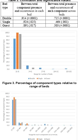
between the total presence and occurrences of each component across beds for all the bed types. These significant correlations demonstrate that the total component occurrences in a bed product increases drastically for every addition of a new component. Figure 3 illustrates that 83% of component types are used in three or fewer double bed designs, while only 10% of component types are used within 4 to 6 double bed designs. Figure 4 points out that 83% of component types have total occurrences of less than or equal to 20. These observations demonstrate that the furniture company does not reuse components effectively across its bed products.
Table 3. Correlation and significance values Bed
type
Between total component presence and occurrences in each
bed
Between total presence and occurrences of each component across
beds Double .914 (<.0001) .715 (<.0001)
Single .924 (.025) .464 (.001)
Guest .891 (.017) .503 (<.0001)
Figure 3. Percentage of component types relative to range of beds
[image:4.612.35.295.461.676.2]Relative commonality (RC)
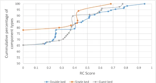
[image:5.612.317.577.74.157.2]Figure 5 presents a plot of the RC score vs the cumulative percentage of component types. The figure shows that on average 70% of component types received a zero RC score across beds (i.e. component presence occurs only once in a bed type). The maximum RC score was associated with a ‘Plastic cap’ component in the double bed family (RC score = 0.944). The RC score for ‘Small screw’ component is only 0.783, which had highest occurrences (i.e. 202 times) and was used across nine double beds. Whereas, the highest scorer ‘Plastic Cap’ had 108 occurrences and was used across 13 double beds. This trend shows that the RC score gives priority to components used across multiple products rather than increasing component occurrences. Also, the RC score penalizes the wider differences of component occurrences across beds. The component ‘Small screw’ only achieved a RC score of 0.783 despite the fact that it was used 50 times in one bed compared to other products that occurred up to 20 times.
Figure 5. Chart between Relative Commonality score and cumulative percentage of component types Degree of Commonality Index (DCI) and Total Constant Commonality Index (TCCI)
The product structure of the bed dataset is flat as there are no sub-assemblies and consequently every component has a single parent in the product structure. Table 4 shows the DCI scores for all bed types. The DCI provides a ratio between the total component occurrences in a product type and the total number of component types. It represents average usage of a component type in each bed type. The DCI score comparison across bed types reveals that the average usage of a component type is better in the Double bed than others. The relative TCCI measure represents the degree to which components are used elsewhere compared to the maximum amount possible. The TCCI scores across bed types illustrate the scope for commonality improvement. However, it is debatable whether high TCCI values truly benchmark against the maximum level of commonality possible.
Table 4. DCI and TCCI scores for all bed types Bed type Number of
components types
Total component occurrences
DCI TCCI
Double 110 2204 20.04 0.950
Single 50 580 11.60 0.915
Guest 78 1183 15.17 0.935
Commonality index (CI)
[image:5.612.319.578.288.389.2]The CI can be interpreted as the ratio between the number of component types and the total number of component presence in a bed type. The higher CI score for the Double bed illustrates they have a low ratio between the number of component types and the total number of component presence (Table 5). The CI score will be higher in a product type if the total number of component presence increases by keeping the number of component types constant.
Table 5. Calculation of CI values for all bed types Bed
type
Number of component types
Maximum number of component presence in a bed
Total number of component presence in a bed type
CI
Double 110 34 238 0.627
Single 50 21 64 0.326
Guest 78 29 116 0.437
Percent Commonality (%C)
[image:5.612.36.292.290.427.2]In this study, only the component commonality percentage is used within the Percent Commonality score (i.e. connection commonality and assembly commonality are not considered). The %C score is less for the Single bed type compared to double and guest types (Table 6). The %C score provides an indicator to increase common components among a bed type.
Table 6. Percent Commonality (%C) score for all bed types
Bed type Number of common components (used in more than one bed)
Number of unique
components (used only in one bed)
%C
Double 38 72 34.5%
Single 11 39 22%
Guest 27 51 34.6%
Product Line Commonality Index (PCI)
[image:5.612.319.577.503.611.2]𝑃𝐶𝐼 =
∑ 𝑛𝑖− ∑ 𝑛1
𝑖 2 𝑃 𝑖=1 𝑃
𝑖=1
𝑃 ∗ 𝑁 − ∑ 1
𝑛𝑖2 𝑃 𝑖=1
∗ 100 (2)
Where P Number of component types that can potentially be standardized in a bed type; N Number of beds in a bed family; ni Number of beds in a bed type that has component i.
[image:6.612.35.294.268.420.2]Table 7 tabulates the PCI scores for the different bed types. The PCI percentage for a product type defines the amount of component types presence across products with reference to maximum possible component commonality index (i.e. P * N). The Guest bed type has a higher PCI percentage than the other two types. The low PCI percentages across all bed types indicate the significant scope for improvement of the level of component presence across beds. Particularly, reducing the component types used only once in a bed will increase the PCI percentages.
Table 7. PCI scores for different bed types
B
ed
ty
pe
Nu
m
ber
o
f
co
m
po
nen
t
ty
pes Num
ber
o
f
bed
s
To
tal
nu
m
be
r
of
co
m
po
ne
nt
ty
pes a
cr
os
s
all
bed
s
∑ 1
𝑛𝑖2 𝑃
𝑖=1
PCI (%)
Double 110 15 238 76.66 10.25
Single 50 5 64 41.33 10.86
Guest 78 6 116 56.49 18.14
Observation on Commonality Measure
The review of the reported commonality metrics (Table 1) and their selected application to a flat-pack product family give rise to the following observations:
A normalized commonality measure that defines levels of design reuse with a relative index between absolute boundaries (e.g. scale of 0 – 1), rather than open or moving boundaries (e.g. DCI measure), simplifies the comparison of designs between product ranges and revisions.
The emphasis of much of the reported work has been to maintain metric consistency in the face of increasing/decreasing product and component types. However the published measures are typically validated on small dataset and consequently their behavior when applied at scale to a product portfolio consisting of many 100s or 1000s of item is not well understood.
High value products are typically assemblies of many sub-assemblies and specialist components consequently it is important that measures characterize commonality at different levels of product structure (i.e. component, assembly, function, within/between product platform and product types) (e.g. %C, PCI, CDI, CMC).
Many of the reported metrics (e.g. CI(C), CDI, CMC) require
multiple factors (i.e. information intensive) to calculate
commonality (i.e. product structures, component costs, materials, manufacturing processes, assembly, end-item volumes, quantities per assembly, and so on). However, to operate at scale (i.e. assess 1000s of product designs) the data required for the calculation should be both readily available and accurate.
Ideally a reuse measure should highlight components whose redesign would have a significant impact on the product’s commonality measure (e.g. expensive, high volume, multi-functional and components used in important products). CI(C) and CMC measures take a component’s cost and
volume information into account. For example, it would be preferable to increase the use of high-volume components across a number of products rather than low-volume components.
Given the above it is obvious that a commonality metric should factor component quantities (i.e. production volume) even if the usage of components is uniform across products.
Metrics that distinguish between differentiating and non-differentiating components can avoid penalizing commonality score when designers deliberately incorporate differentiating factors (e.g. PCI, CDI, TCI).
Most of the metrics focused solely on identifying commonality at the different levels of product family structure. However, very few give insights into the implicit trade-offs that exists between commonality and variety across a product type (e.g. CDI). This line of research enquiry is important because commonality may have adverse impacts on design efficiency (for instance when extreme standardization results in excessive functionality [16]).
The flat-pack furniture case study highlights the importance of two critical parameters in the calculation of commonality metrics:
The number of component presence across products
The number of component types
Likewise important parameters not considered in reported metrics are:
The concentration of component occurrences among substitutable component
The number of alternative components
The degree of product variety
A PROBABILISTIC DESIGN REUSE INDEX
We propose to characterize the extent to which an organization is reusing components within products using the concept of a Purely random design mechanism (PRDM). To make the comparison meaningful, we organize components into families where to facilitate the analysis it is assumed that components are substitutable for each other within a family. As such, the PRDM is equally likely to choose any family member (e.g. any bolt, and bearing) when such a component is required as opposed to an organization that is highly effective with reuse demonstrating a higher concentration of use on fewer components. We are effectively comparing the difference between two probability distributions. The hypotheses motivating this comparison is that the best performing organizations concentrate all reuse on one member of each family and the poorest make equal use of all family members.
We do not directly observe an organization’s probability distribution for component selection, only the frequency in which components have been selected. Assuming that component selection is independent of past product choices, and the probability of a component being selected is the same for all products then we have a multinomial distribution [17] to describe the randomness of the data.
Specifically, we use ‘c’ to denote the number of families within the comparator set, denoting the total number of products with ‘m’. For each family of components ‘i’ we denote with ‘ni’ the number of options, i.e. members of the family. We denote with ‘pij’ the conditional probability that component ‘j’ from family ‘i’ is selected given a component from family ‘i’ is selected for a particular product. We denote the observed number of selections of component ‘j’ from family ‘i’ with ‘xij’. ‘P’ represents the matrix of probabilities ‘pij’ and the Likelihood function for the data, i.e. the probability of observing the data as a function of the conditional probabilities, is expressed in Eq. 3.
𝐿(𝑃) ∝ ∏ ∏ 𝑝𝑖𝑗𝑥𝑖𝑗 (3)
𝑛𝑖
𝑗=1 𝑐
𝑖=1
𝑠. 𝑡. ∶ ∑ 𝑝𝑖𝑗 = 1, ∀𝑖 𝑛𝑖
𝑗=1
While we do not directly observe ‘P’ we can make inferences. The Maximum Likelihood Estimate (MLE), i.e. the value of the conditional probabilities that would most likely result in the observed data, denoted by 𝑃̂ has elements expressed in Eq. 4.
𝑝̂𝑖𝑗 =
𝑥𝑖𝑗
∑ 𝑥𝑖𝑗
𝑛𝑖 𝑗=1
(4)
The PRDM has 𝑝𝑖𝑗𝑃𝑅𝐷𝑀= 1
𝑛𝑖 and as we increase the number of products, i.e. ‘m’, the estimates 𝑝̂𝑖𝑗will converge with the true
underlying probabilities for the organization, i.e. ‘𝑝𝑖𝑗’. We seek
a measure for the difference between 𝑝̂𝑖𝑗and 𝑝𝑖𝑗𝑃𝑅𝐷𝑀for ∀𝑖, 𝑗. The
Kullbeck-Leibler divergence measure [18] provides a means to measure the difference between distributions and is expressed in Eq. 5 for family ‘i'.
𝐷𝑖= ∑ 𝑝̂𝑖𝑗ln (
𝑝̂𝑖𝑗
𝑝𝑖𝑗𝑃𝑅𝐷𝑀
)
𝑛𝑖
𝑗=1
(5)
If 𝑝̂𝑖𝑗 = 𝑝𝑖𝑗𝑃𝑅𝐷𝑀 for all options ‘j’ then Di = 0 and as the
difference grows so does Di. This measure can be re-expressed as a ratio of Likelihood functions, so the difference between the observed frequencies and the PRDM is measured relative to the probability of having generated the observed data. If the observed frequencies are not consistent with PRDM then this measure will be large. This is derived in the following Eq. 6.
^
1
^
ln
ln
ij i
x n
ij PRDM
i ij
i
i
ij
PRDM ij
i
p p D
n L p L p
n
(6)
Asymptotically, when there a large number of products the value of this measure is characterized with the χ2 distribution when the differences are due to sampling variation only, i.e.
𝑝𝑖𝑗 = 𝑝𝑖𝑗𝑃𝑅𝐷𝑀. This result can be used to map the distance
measure to a scale between 0 and 1 and facilitate interpretation. Specifically, as ‘m’ tends to infinity, under the null hypothesis 𝑝𝑖𝑗= 𝑝𝑖𝑗𝑃𝑅𝐷𝑀 then
−2 ln (𝐿(𝑃)
𝐿(𝑃)̂) = −2 ∑ ∑ 𝑥𝑖𝑗 (ln (∑ 𝑥𝑖𝑗 𝑛𝑖
𝑗=1
) − ln(𝑥𝑖𝑗) − ln(𝑛𝑖)) 𝑛𝑖
𝑗=1
𝑐
𝑖=1
(7)
has a χ2 distribution with ∑ 𝑛
𝑖− 𝑐 𝑐
𝑖=1 degrees of freedom [20].
Performance of PDRI with Few Designs
The use of the measure χ2 distribution is justified using asymptotic theory for a large number of products. For situations with few products, this distributional assumption would not be appropriate, and a simulation exercise would be required. For small samples we would caution using this for strict hypothesis testing as the actual significance level attached to the test would be different from the value obtained from the χ2 distribution. However, even with few products the measure with the χ2 distribution can still be used as a measure of distance with the PRDM; it will be a monotonic transformation of the true CDF value and as such if an organization were to score higher than another using the χ2 distribution this ranking would be maintained with the true CDF evaluation.
We conducted a simulation study using Maple 2017 [20]. The following three parameters were controlled for in the study: number of products i.e. m = 3..10, number of families i.e. c = 3..10 and number of family members (options) i.e. n = 3..10. For each set of parameters 200 simulations were realized and the empirical CDF was compared with the corresponding χ2 CDF. The difference between the CDF’s (empirical minus χ2) were assessed and the following summary measures produced: maximum difference, minimum difference, median difference as well as the correlation between the two CDF’s. A sample of these results are provided in Annex – A.
From Annex – A it can be observed that while the correlation coefficient is high (typically above 0.9) there can be aspects where the CDF’s are far apart, but the difference generally decreases with more products. Moreover, the χ2 CDF is typically greater than then empirical CDF evaluated at the same value as observed from the large negative numbers on the minimum difference column.
We conducted a second simulation study to assess the 95th
percentiles. Specifically, for situations where the χ2 CDF was below or above its 95th percentile, we assessed whether the
empirical distribution was above or below its 95th percentile.
The results are provided in Table 8 and for this simulation 10000 runs were performed for each parameter combination. Upon inspection of Table 8 it can be observed that if the χ2 CDF is below the 95th percentile, then the empirical was as well.
However, even with designs of 100, agreement above the 95th
percentile is questionable. This would be relevant if the measure was to be used in the form of a hypothesis test, suggesting the χ2 test is more accurate when accepting the null hypothesis than when rejecting it.
[image:8.612.343.519.423.558.2]In sum, if the χ2 analysis show no significant difference then the true CDF evaluation which is more computationally expensive would conclude similarly, however if the χ2 analysis suggests a significant difference the true CDF evaluation may differ. This is only a problem if the analysis is being used as a strict hypothesis test rather than as a distance measure.
Table 8 Sample of results from simulation exercise to assess the difference between the 95th percentile of the
2 and the true distribution of the statistic (Eq. 7)Op
tio
ns
Fam
ilies
Pro
du
cts
P.E. is < 0.95 given
2
is < 0.95P.E. > 0.95 given
2
is > 0.95 (P.E. Probability Empirical)3 3 50 1 0.9560
5 5 50 1 0.7937
7 7 50 1 0.7143
10 10 50 1 0.4980
3 3 100 1 0.9960
5 5 100 1 0.8591
7 7 100 1 0.8726
10 10 100 1 0.7375
Best and No Reuse Mechanisms
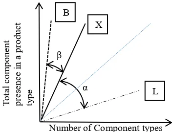
The Purely random design mechanism (PRDM) is a concept developed to provide a benchmark for assessing the concentration with which components are reuse within families. The PRDM is instructed to select components from a defined list and does so at random with components being equally likely to be selected. The χ2 value provides a measure of the distance an organization is from the PRDM. However, the PRDM is not the most inefficient mechanism. The No-Reuse Mechanism (NRM) characterises a designer that never visits the catalogue of historical products and consequently every new product they create is entirely original with no reuse.
Figure 6 Relationship between an organization’s components reuse (X) compared with minimal reuse
where new components are created for each new product (L) and best reuse where common components are used in every product (B) Figure 6 illustrates the relationship between an organization (labelled X), number of component types and the total component presence in a product type. An efficient organization generates many products from few components and as such the steeper the slope the more efficient the organization. There is a lower limit on the slope of this relationship; as NRM (labelled L) always creates new components for each new product then
Number of Component types
T
otal
co
m
po
nen
t
pr
esen
ce
in
a
pr
od
uct
ty
pe α
X
L B
NRM lines will not exceed the 45 degree line and as more components are designed the slope will become flatter. The angle ‘α’ (known as the “healthier” angle) between the NRM line (L) and an organization’s line (X) provides a measure of re-use (i.e. larger the value of α the healthier to levels of reuse). To calculate the slope of the NRM line, the number of component types was calculated by multiplying an average number of component types in a product and the number of products in a product family. Whereas, for Best Reuse Mechanism (BRM), the number of component types is equal to an average number of component types in a product. The improvement angle ‘β’ is the difference between best the BRM line (B) and the current organization line (X). These reference angles for a single product type are illustrated in Fig. 6. The figure is not aimed to depict reference angles for all product types together.
RESULTS
[image:9.612.34.297.431.538.2]Structurally similar components (e.g. hinges, dowels, cam lock nuts etc.) from the furniture dataset were organized into families to allow application of the proposed PDRI measure. Although not all structurally similar components will be “substitutable” in practice, by assuming they could be, the PRDM can be used to focuses design reviews that require differences to be justified. Table 9 summarizes the number of products, families and average number of options for each bed type. It should be noted that only families with more than one option are considered in this reuse calculation. The total number of such families is higher for the Double bed, whereas the average number of options is higher for the Guest bed type.
Table 9 Distribution of number of products, families and average number of options per bed type Bed type No. of
beds Total number of families
No. of families with more than one option
Average number of options per family
Double 15 40 22 4.3
Single 5 22 11 3.5
Guest 6 33 11 5.1
The χ2 distribution value for all bed types is one. The high
score demonstrates that the furniture company, at the aggregated level, used a higher concentration of use on fewer component options within the families; unlikely the Purely random design mechanism (PRDM) which would have chosen all the components equally often. The high differentiation between probability distributions shows that the probability distribution of component usage in the furniture company is different to PRDM at the overall level.
The χ2 distribution value for each family was calculated to
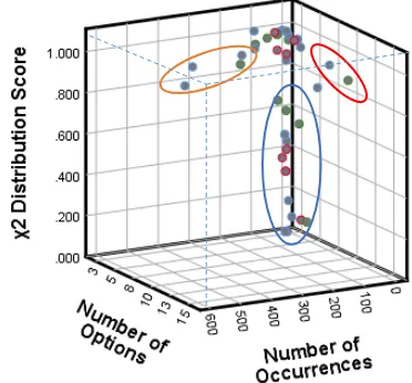
understand the variation individually with reference to PRDM. Figure 7 represents 3D scatter plots between χ2 distribution value
for each family with reference to the number of options and the total component occurrences in the family. The advantage of this χ2 distribution value is that it accounts for sample size (i.e.
considering a cumulative number of options). The results show that 64% of families in the Single bed type have a χ2 score less than 0.95 but only 36% for the Double and Guest bed types. This finding demonstrates that most of the families in the Single bed type have trended towards random component selection leading to the equal use of all family members. Thus there is significant opportunity to increase the higher concentration of use on fewer components within the Single bed type.
The three elliptical zones shown in Fig. 7 represent groups of component family within which it is most likely that component reuse improvements can be made:
Blue zone identifies emerging or rare families with very low χ2 values. This zone has few options and occurrences in a family. Consider for example a component type that is rarely used; it will not find itself with a high score as it hasn’t demonstrated itself as being significantly different from the PRDM. Among the component families with less than 0.95 χ2 score, 88% have only fewer than four options. Therefore, this zone contains a significant number of families that behaves similarly to PRDM.
Red zone identifies matured families with many available options. All families with a high number of options have greater than 0.95 χ2 values. However, the families in this zone should the focus of initiatives to reduce/eliminate the available options.
Orange zone identifies the high component occurrence families. Again all families with high component occurrences have greater than 0.95 χ2 values. The focus in the region is to reduce component occurrences spread across available options.
These three zones with different χ2 distribution values help to prioritize which families to investigate first. Increasing component reuse in these different zones will have different overall reuse and business impact.
Figure 7 3D scatter plot of χ2 distribution value, number of options and total occurrences for each
component family
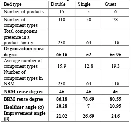
[image:9.612.352.538.470.643.2]benchmark an organization’s reuse performance, No Reuse Mechanism (NRM) and Best Reuse Mechanism (BRM) were generated. Table 10 summarizes the so called, Healthier angle, (α) and the Improvement angle (β) along with calculated parameters for all bed types. The Double bed has a better Healthier angle (α) and low improvement angle (β). Whereas, the Single bed has a low Healthier angle (α) and high improvement angle (β). The avoidance of subjective information in calculating is the primary advantage of these angles.
Table 10 Furniture organization, Best and No-Reuse Mechanisms Angle calculation
Bed type Double Single Guest
Number of products 15 5 6
Number of
component types 110 50 78
Total component presence in a
product family 238 64 116
Organization reuse
degree 65.16 52 55.95
Average number of
component types 15.9 12.8 19.3
Number of
component types in
NRM 238 64 116
NRM reuse degree 45 45 45
BRM reuse degree 86.18 78.69 80.55
Healthier angle (α) 20.28 7 10.95
Improvement angle
(β) 21.02 26.69 24.6
DISCUSSION
Table 11 summarizes six commonality index values for the three-bed types. The different commonality index values provide different information about the degree of commonality across the bed types. The Double bed family has a better degree of commonality than the other two types across all the commonality indexes, except for the PCI values where the Guest bed type has a higher score.
Table 11. Summary of the commonality index values Bed
type Max. RC DCI TCCI CI %C PCI Double 0.944 20.04 0.950 0.627 34.5% 10.25% Single 0.682 11.60 0.915 0.326 22% 10.86% Guest 0.773 15.17 0.935 0.437 34.6% 18.14% The interpretations drawn from these values help to answer the following questions:
Which component type has a high probability of presence across beds? (RC)
On average, how many times has a component been used in a bed type? (DCI and TCCI)
What is the ratio between component types and the total number of component presence in a bed type? (CI)
What is the percentage of common and unique components in a bed type? (%C)
What is the percentage of total component presence to the maximum possible component commonality for a bed family? (PCI)
Other than the RC score, all other measures provide different, aggregated interpretations of commonality score. The RC score provides individual component sharing across products. In contrast the new PDRI commonality measure presented here answers the following questions:
Which component families deviate most from a Purely random design mechanism (PRDM)?
What are the best and worst component families (from a reuse perspective) in a product type?
How to categorize component families into different zones based on the PRDM, the number of options and the total component occurrences in each family?
How does component reuse in an organization compare with the extremes of No Reuse Mechanism (NRM) and Best Reuse Mechanism (BRM)?
The answers to these questions will help focus (i.e. prioritize) an enterprise’s engineering effort on individual component families for reuse improvements, rather than providing aggregated reuse value. The proposed measures objectively quantify levels of reuse and so aid understanding of component frequency distribution within a family. In other words it can help to increase occurrences of few components in a family, which will eventually lead to reducing the number of options and component types.
The visualization of a component family’s deviation from the random mechanisms in a 3D scatter plot illustrates one way in which the proposed approach can be used to identify targets for redesign to improve reuse. The concepts of the healthier and improvement angles do not rely on subjective information and significantly reduces the calculation effort required to generate them. In the case study these angles illustrate that the Double bed type is better than the Single bed type in reuse measures. It is interesting to note that this finding agrees with the results of other published metrics (Table 11).
CONCLUSION
number of component options and occurrences. This reuse measure along with the No-reuse and the Best-reuse mechanisms provide clear benchmark references for organization to track improvement progression of component reuse.
The authors’ ongoing work aims to demonstrate the efficiency of these measures on larger industrial data sets. Particularly, the focus is to demonstrate these metrics at the different product structure levels. In the long term the efficiency of these metrics needs to be tested in industrial environments to quantify the labor required to apply the measures in practice. While avoiding subjective measures the researchers will also investigate how other information (such as component costs, materials and volumes) can be incorporated into the metric to better reflect the context and implications of reuse levels. ACKNOWLEDGEMENT
This work was supported by Engineering and Physical Sciences Research Council, UK [grant number EP/R004226/1]. A dataset supporting this research and the process to calculate the proposed probabilistic based measure is openly available from http://dx.doi.org/10.15129/20ac02c9-7c33-4c5a-a436-157af53ff123
REFERENCES
[1] Hou, Suyu, and Karthik Ramani. "Dynamic query interface for 3D shape search." In ASME 2004 International Design Engineering Technical Conferences and Computers and Information in Engineering Conference, pp. 347-355. American Society of Mechanical Engineers, 2004.
[2] Schacht, Silvia, and Alexander Mädche. "How to prevent reinventing the wheel?–design principles for project knowledge management systems." In International Conference on Design Science Research in Information Systems, pp. 1-17. Springer, Berlin, Heidelberg, 2013. [3] Moscato, Donald R. "The application of the entropy
measure to the analysis of part commonality in a product line." The International Journal of Production Research 14, no. 3 (1976): 401-406.
[4] Collier, David A. "The measurement and operating benefits of component part commonality." Decision Sciences 12, no. 1 (1981): 85-96.
[5] Wacker, John G., and Mark Treleven. "Component part standardization: an analysis of commonality sources and indices." Journal of Operations Management 6, no. 2 (1986): 219-244.
[6] Martin, Mark V., and Kosuke Ishii. "Design for variety: development of complexity indices and design charts." In Proceedings of, pp. 14-17. 1997.
[7] Siddique, Zahed, David W. Rosen, and Nanxin Wang. "On the applicability of product variety design concepts to automotive platform commonality." In ASME Design Engineering Technical Conferences-Design Theory and Methodology. 1998.
[8] Kota, Sridhar, Kannan Sethuraman, and Raymond Miller. "A metric for evaluating design commonality in product
families." Journal of Mechanical Design 122, no. 4 (2000): 403-410.
[9] Jiao, Jianxin, and Mitchell M. Tseng. "Understanding product family for mass customization by developing commonality indices." Journal of Engineering Design 11, no. 3 (2000): 225-243.
[10]Alizon, Fabrice, Steven B. Shooter, and Timothy W. Simpson. "Assessing and improving commonality and diversity within a product family." Research in Engineering Design 20, no. 4 (2009): 241.
[11]Thevenot, Henri J., and Timothy W. Simpson. "A comprehensive metric for evaluating component commonality in a product family." Journal of Engineering Design 18, no. 6 (2007): 577-598.
[12]Blecker, Thorsten, and Nizar Abdelkafi. "The development of a component commonality metric for mass customization." IEEE Transactions on Engineering Management 54, no. 1 (2007): 70-85.
[13]Sinigalias, Pavlos Christoforos, and Argyris Dentsoras. "Index-based metrics for the evaluation of effects of custom parts on the standardization of mechanical systems." In DS 80-7 Proceedings of the 20th International Conference on Engineering Design (ICED 15) Vol 7: Product Modularisation, Product Architecture, systems Engineering, Product Service Systems, Milan, Italy, 27-30.07. 15. 2015. [14]Simpson, Timothy W. "Product family and product platform
benchmarking with commonality and variety indices." In ASME 2017 International Design Engineering Technical Conferences and Computers and Information in Engineering Conference, pp. V02BT03A041-V02BT03A041. American Society of Mechanical Engineers, 2017.
[15]Xiaoli, Ye, J. Thevenot Henri, Alizon Fabrice, K. Gershenson John, and W. Simpson Timothy. "A quantitative representation of the tradeoff between product commonality and variety in product family design." Guidelines for a Decision Support Method Adapted to NPD Processes (2007).
[16]Thomas, Lawrence Dale. "Functional implications of component commonality in operational systems." IEEE transactions on systems, man, and cybernetics 22, no. 3 (1992): 548-551.
[17]Johnson, Norman Lloyd. Discrete multivariate distributions. No. 04; QA273. 6, J645. 1997.
[18]Kullback, Solomon, and Richard A. Leibler. "On information and sufficiency." The annals of mathematical statistics 22, no. 1 (1951): 79-86.
[19]Lawless, Jerald F. Statistical models and methods for lifetime data. Vol. 362. John Wiley & Sons, 2011.
ANNEX A
A sample of results from simulation exercise to assess the difference between the
2and the true distribution ofthe statistic (Eq. 7)
Options Families Products Max Min Median Correlation
3 3 3 0.0340 -0.3940 -0.1336 0.9359
3 3 4 0.0650 -0.2673 -0.1200 0.9605
3 3 5 0.0491 -0.2513 -0.1145 0.9716
3 3 6 0.0461 -0.2147 -0.0968 0.9805
3 3 7 0.0728 -0.1159 -0.0164 0.9934
3 3 8 0.0316 -0.1579 -0.0790 0.9905
3 3 9 0.0047 -0.1511 -0.0746 0.9918
3 3 10 0.0217 -0.1110 -0.0542 0.9943
5 5 3 0.0461 -0.4252 -0.2309 0.9603
5 5 4 0.0117 -0.4431 -0.2298 0.9527
5 5 5 0.0045 -0.3745 -0.2593 0.9479
5 5 6 0.0037 -0.3353 -0.2271 0.9590
5 5 7 0.0019 -0.2963 -0.2143 0.9632
5 5 8 0.0012 -0.2317 -0.1521 0.9785
5 5 9 0.0008 -0.2404 -0.1810 0.9724
5 5 10 0.0016 -0.2091 -0.1559 0.9832
7 7 3 0.1579 -0.3034 -0.0401 0.9768
7 7 4 0.0377 -0.4475 -0.2391 0.9453
7 7 5 0.0095 -0.4452 -0.2577 0.9537
7 7 6 0.0015 -0.4528 -0.2714 0.9505
7 7 7 0.0018 -0.4579 -0.3214 0.9309
7 7 8 0.0015 -0.3763 -0.2804 0.9539
7 7 9 0.0025 -0.3973 -0.2779 0.9331
7 7 10 0.0019 -0.4029 -0.2945 0.9165
10 10 3 0.5318 -0.0881 0.2542 0.9491
10 10 4 0.2098 -0.2459 -0.0065 0.9878
10 10 5 0.0793 -0.3317 -0.1555 0.9755
10 10 6 0.0290 -0.4325 -0.2567 0.9501
10 10 7 0.0060 -0.4888 -0.3124 0.9258
10 10 8 0.0017 -0.5144 -0.3666 0.9212
10 10 9 0.0013 -0.4923 -0.3513 0.9020
![Figure 2. Sample Product Family Evaluation Graph along with the angle factor [15]](https://thumb-us.123doks.com/thumbv2/123dok_us/1422913.94987/3.612.321.570.297.692/figure-sample-product-family-evaluation-graph-angle-factor.webp)