Integrating QTL analysis into plant breeding practice using Bayesian statistics

2008

Integrating QTL analysis into plant breeding

practice using Bayesian statistics

Shengqiang Zhong

Iowa State University

Follow this and additional works at:https://lib.dr.iastate.edu/rtd

Part of theAgricultural Science Commons,Agronomy and Crop Sciences Commons,

Biostatistics Commons, and theGenetics and Genomics Commons

This Dissertation is brought to you for free and open access by the Iowa State University Capstones, Theses and Dissertations at Iowa State University Digital Repository. It has been accepted for inclusion in Retrospective Theses and Dissertations by an authorized administrator of Iowa State University Digital Repository. For more information, please [email protected].

Recommended Citation

Zhong, Shengqiang, "Integrating QTL analysis into plant breeding practice using Bayesian statistics" (2008).Retrospective Theses and Dissertations. 15868.

Integrating QTL analysis into plant breeding practice using Bayesian statistics

by

Shengqiang Zhong

A dissertation submitted to the graduate faculty

in partial fulfillment of the requirements for the degree of

DOCTOR OF PHILOSOPHY

Major: Genetics

Program of Study Committee: Jean-Luc Jannink, Co-major Professor Jack C. M. Dekkers, Co-major Professor

Alicia L. Carriquiry Michael Lee Rohan L. Fernando

Jode W. Edwards

Iowa State University

Ames, Iowa

2008

3307036

TABLE OF CONTENTS

ACKNOWLEGDEMENTS...v

ABSTRACT... vi

CHAPTER I. INTRODUCTION...1

Genetic Markers...1

Marker Assisted Selection for Qualitative Traits...3

Marker-assisted Backcrossing ...3

Gene Pyramiding ...4

Marker Assisted Selection for Quantitative Traits...5

Limitations of Current MAS...5

Statistical Developments of QTL Analysis...6

Association Analysis...8

Dissertation Organization ...10

References...13

CHAPTER II. COMPARISON OF TWO MATING DESIGNS FOR MULTIPLE-FAMILY QTL MAPPING...19

Abstract ...19

Introduction...20

Methods...22

Results...26

Discussion...27

References...29

Figures...32

Figure 1. QTL detection power under different arbitrarily threshold...33

Figure 2. Mean square error of posterior QTL allelic variance ...34

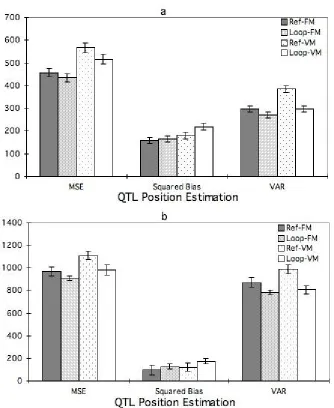
Figure 3. Mean square error of QTL position estimation ...35

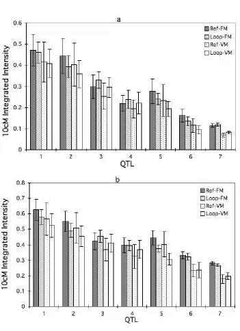
Figure 4. Average of 10 cM integrated intensity across replicate simulations...36

CHAPTER III. USING QTL RESULTS TO DISCRIMINATE AMONG CROSSES BASED

ON THEIR PROGENY MEAN AND VARIANCE...38

Abstract ...38

Introduction...39

Theory...42

Simulations ...47

Results...49

Discussion...51

Acknowledgments...55

Literature Cited ...56

Tables...60

Table 1. Inbred progeny frequencies and genotypic values...60

Table 2. Three possible cross types and their frequencies...60

Figures... 61

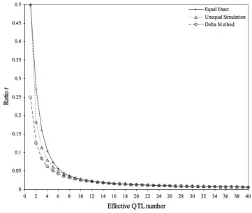
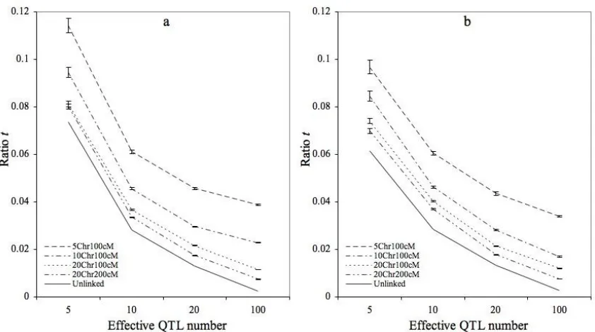
Figure 1. Ratio t for independent QTL ...62

Figure 2. Ratio t for different genome sets ...63

Figure 3. Correlations from random crosses...64

Figure 4. Correlations from top forty parent crosses ...65

CHAPTER IV. ASSOCIATION-BASED GENOMIC SELECTION IN CULTIVATED BARLEY...66

Abstract ...66

Introduction...67

Materials and Methods...69

Results...72

Discussion...75

Literature Cited ...79

Table ...81

Table 1. Two-row spring barley lines ...81

Figures... 82

Figure 2. Decline of LD as measured by r ) 2 against distance...84

Figure 3. Decline of the moving-average LD against distance in cM ...85

Figure 4. Correlation between simulated and predicted breeding values ...86

Figure 5. Prediction accuracy with different population sizes...87

Figure 6. Posterior probabilities under observed causal SNP condition...88

Figure 7. Posterior probabilities under unobserved causal SNP condition...89

CHAPTER V. GENERAL CONCLUSIONS...90

References...93

APPENDIX. R CODE FOR GENOMIC SELECTION ...94

Bayes-A (Meuwissen et al. 2001; Xu 2003; ter Braak et al. 2005) ... 94

Bayes-B (Meuwissen et al. 2001) ... 97

ACKNOWLEDGEMENTS

I want to take this opportunity to thank all people who helped me during my Ph.D. study. It is not possible for me to list all the names here and I apologize in advance if omit someone’s name.

My extremely grateful thanks go to my advisors Dr. Jean-Luc Jannink and Dr. Jack Dekkers for their guidance, patience and support. Dr. Jannink was very understanding and always available for great instruction, and encouragement throughout my Ph.D. study. My whole thesis has benefited enormously from Dr. Jannink’s sharp insight in scientific research and from his extensive knowledge in quantitative genetics. Dr. Dekkers provided a new perspective and invaluable suggestion to my study. I would like to thank other committee members Dr. Alicia L. Carriquiry, Dr. Michael Lee, Dr. Rohan L. Fernando and Dr. Jode W. Edwards for their advice and support from various aspects.

I want to thank the students in the Jannink’s Lab: Murli Gogula, Jin Long, Alona Chernyshova, Yoon-Soup So, Massiel Orellana, and Julia Olmstead and Lucía Gutiérrez for all their support and sharing the fun time in the field. I am thankful to George Patrick and Ron Skrdla from Jannink’s group for sharing field breeding experience. I also want to thank the researchers from the genomic selection group in the Animal Science Department for sharing their experience.

I would like to express my appreciation to all the faculty members, students and staffs in the Agronomy Department for providing me with such a professional research environment.

ABSTRACT

CHAPTER I. INTRODUCTION

Traditional plant breeding has depended on phenotypic selection for agronomically important traits. Significant crop improvements through phenotypic selection have been made (Fehr, 1984). However phenotypic selection in some situations presents difficulties due to genotype-environment interactions and unreliable, or expensive phenotyping. With recent considerable marker technology developments, molecular marker-assisted selection (MAS), that is, selection for the genetic determinant or determinants of a trait of interest based on marker genotypes, offers a great opportunity for efficient selection for traits controlled both by major genes as well as by many quantitative trait loci (QTL). In this chapter, I first briefly review genetic markers, MAS for qualitative traits, and MAS for quantitative traits. Then I place the research described in this thesis against this background.

Genetic Markers

Genetic markers can be classified into three major groups: phenotypic markers, biochemical markers and DNA sequence based markers. Phenotypic markers are generally visually characterized morphological characters, such as pea flower color and seed shape determined by Mendelian genes. Some phenotypic markers are easy to score and if they are linked to important agricultural traits such as disease resistance, they can be used in breeding programs (Joshi et al 2004). Biochemical markers, mostly isozyme markers, usually exploit different variants of the same enzyme (Weeden and Wendel, 1990). Phenotypic and biochemical markers are limited in number and might be subjected to variation due to environment or developmental stage, so their application in breeding is restricted (Winter and Kahl, 1995).

polymorphisms (SNPs). The RFLP is the oldest type of DNA marker. Large amounts of DNA are typically required for RFLP detection and it is difficult to automate the analysis (Erlich and Arnheim, 1992). Other types of molecular markers generally require smaller amounts of DNA. The RAPD, which utilizes single primers of arbitrary sequence to generate strain-specific arrays of anonymous DNA fragments by low stringency PCR amplification (Wang et al 1993), is relatively unreliable in terms of reproducibility. The AFLP requires DNA digestion by restriction enzymes, then using PCR with selective primers to amplify specific fragments (Vos and Zabeau, 1993). The SSR is based on short-repeat sequences that are widely dispersed throughout the eukaryotic genome. SSRs are highly informative because their mutation mechanism generates variable numbers of repeats, and thus many different marker alleles are possible. A SNP marker is a difference in nucleotide between different alleles, at a single base pair position in the genome. Due to the abundance of SNPs and the development of sophisticated high-throughput of SNP detection systems, SNP usage has increased in QTL mapping and MAS. Continuously decreasing SNP cost will likely remove this important factor that limits MAS implementation.

The development of abundant DNA markers has made many marker applications possible: estimation of genetic diversity (Smith et al 2000), germplasm characterization (Mason et al 2005), construction of linkage maps (Luo et al 2001), qualitative gene and QTL mapping, the discovery of useful candidate genes (Thornsberry et al 2001; Blair et al 2003), and MAS (Brahm et al 2000; Willcox et al. 2002).

For breeding purposes, molecular markers can be applied in several ways: 1) Marker-assisted backcrossing (Willcox et al. 2002).

2) Gene pyramiding (Servin et al. 2004).

3) Selecting superior individuals within a population based on marker-estimated breeding values (Lande and Thompson 1990; Meuwissen et al. 2001).

4) Selecting best crosses among a set of lines (Zhong and Jannink, 2007).

(Lewontin and Kojima, 1960). Linkage disequilibrium in the population is mainly generated by mutation, selection, drift and migration, and dissipated by recombination (Falconer and Mackay, 1997). Existent LD will remain for many generations between tightly linked loci and decay over few generations for loosely linked or unlinked loci. Three kinds of markers can be distinguished based on LD of the markers with the loci that contribute to genetic variation for the trait in the population (Dekkers, 2004):

i) The molecular marker itself is the functional polymorphism, which is the most favorable situation for MAS. In this case, it could be ideally referred to as gene-assisted selection. While this kind of relationship is the most preferred one, it is also difficult to find this kind of markers.

ii) The marker is in LD with the functional mutation throughout the population. Population-wide LD can usually be found when markers and genes of interest are physically close to each other. Selection using these markers can be called LD-MAS.

iii) The marker is in linkage equilibrium (LE) with the functional mutation across the population. This is the most difficult and challenging situation for QTL mapping and MAS. Although a marker and a linked QTL may be in LE across the population, within a family LD will always exist, even between loosely linked loci. Within-family LD can be used to detect QTL and for MAS (Fernando and Grossman, 1989).

Marker Assisted Selection for Qualitative Traits

Marker-assisted Backcrossing

In conventional backcrossing programs using phenotypes, a minimum of five or six-backcrossing generations is required to transfer the desired allele and recover the recurrent background. Furthermore there is a risk linkage drag around the target gene, that is, that a large segment of the donor-parent genome will remain intact around the target gene. The expected proportion of the recurrent parent background genome is 1 – (1/2)t+1 after backcrossing for t generations. However, any specific backcross progeny will vary from this expectation due to chance. Background markers can identify progeny more similar to the recurrent parent and thus accelerate the recovery of recurrent parent genotype. Frisch et al (1998) used simulations to compare several different backcrossing strategies in terms of how quickly they recovered a large proportion of the recurrent parent genotype. They recommended a four-step sampling strategy to quickly recover the recurrent parent genotype, which includes: (1) selecting individuals carrying the target allele; (2) selecting individuals homozygous for the recurrent parent alleles at loci flanking the target locus; (3) selecting individuals homozygous for recurrent parent alleles at remaining loci on the same chromosome as the target allele; and (4) selecting one individual that is homozygous for recurrent parent alleles at most loci (across whole genome) among those that remain. They found that using this strategy one could expect the recovery of at least 96% of the recurrent parent genotype with 90% probability after three generations of backcrossing with a reasonable population size (50-100).

Chen et al. (2000) demonstrated a very good example of marker-assisted backcrossing. They improved the bacterial blight resistance of an elite rice line by introgressing Xa21, a wide-spectrum bacterial blight resistance gene, into this line by molecular marker-assisted backcrossing. They selected for target alleles at two markers tightly linked to Xa21 and for recurrent parent alleles at flanking markers outside of the gene region to decrease linkage drag during three backcross generations. In the third backcross generation, they used 128 RFLP markers for background selection and recovered a line that was essentially identical to the recurrent parent cultivar, but possessing the Xa21 allele.

Gene Pyramiding

to enhance resistance to disease and insects by selecting for two or more than two genes at a time. The advantage of using markers in this case is that it allows the breeder to select for QTL-alleles that have same phenotypic effect, which can be nearly impossible with conventional breeding approaches. For example, due to the broad spectrum of blast resistance of Xa21 allele, a breeding line with Xa21 only cannot be distinguished from a breeding line with Xa21 and some other genes with similar resistance by conventional phenotypic approach. Using MAS, Singh et al (2001) pyramided three bacterial blast resistance genes (Xa5, Xa13 and Xa21) into an indica rice cultivar. Pyramiding of several resistance genes by marker-assisted breeding may lead to more durable resistance.

Marker Assisted Selection for Quantitative Traits

Lande and Thompson (1990) showed in their original paper how DNA marker information could improve estimates of breeding values for quantitative traits. Their essential requirement was that the observable markers be in LD with the unobservable QTL affecting the trait. Many important agricultural traits, such as yield, are under polygenic control with gene interactions (epistasis), strong environmental influence, and genotype-by-environment interaction on trait expression. Although MAS has been widely implemented for traits controlled by major genes using introgression and gene pyramiding, successful application of MAS to quantitative traits has been limited.

Limitations of Current MAS

between the marker and the QTL would generally not be consistent from family to family. The consequence of inconsistency of marker-QTL linkage phase is that estimated marker allele effects would be only nested within family and meaningless across families. Fernando and Grossman (1989) developed QTL mapping and MAS with LE markers by modeling the co-segregation of markers and QTL within pedigree or family. Research in overcoming this second limiting factor (lack of marker density) is not the subject presented here. Rather, we simply take for granted that markers at high density are available such that markers exist that are in population-wide LD with QTL. In that case, marker-QTL phases are consistent across individuals and it becomes reasonable to estimate marker allele effects. In other words, we assume now that we are proceeding with LD-MAS in the sense of Dekkers (2004).

Statistical Developments of QTL Analysis

The primary problem of QTL analysis with high-density marker data is that the number of independent variables (i.e., the number of markers) is large relative to the number of observations (i.e., the number of genotypes observed). Several variable selection strategies have been developed and applied to address this problem. Step-wise regression is a common procedure for variable selection for multiple QTL analysis in composite interval mapping (Jansen1993; Zeng 1994) and multiple-interval mapping (Kao et al. 1999). The QTL effects are treated as fixed effects in step-wise regression. After a single locus model is fitted, the residuals are examined for the presence of a second QTL, and so on. A drawback of step-wise regression is that effects are included and removed from the model according to somewhat arbitrary statistical thresholds. Because many markers are tested in QTL mapping, the process necessarily entails relatively stringent significance thresholds for marker inclusion in the model. The result is that too few QTL are identified as significant in a mapping population, and the effects of those identified QTL are overestimated (Beavis, 1994; Beavis 1998; Schön et al., 2004; Xu 2003a). In addition, the QTL that exceed the chosen significance threshold often jointly only account for a limited proportion of the genetic variance. All these issues limit the scope and potential impact of MAS based on QTL analysis by step-wise regression.

1997; Sillanpaa and Arjas 1998). Similarly, Yi et al. (2003) applied a stochastic search variable selection (SSVS, a Bayesian variable selection via Gibbs sampler) method to QTL analysis. One advantage of the Bayesian approach is that it considers the marginal posterior distributions of all parameters, including QTL position and effects given the data (Satagopan et al 1996).

New developments in shrinkage estimation seek to avoid variable selection by including all markers as predictors in the model and shrinking the estimated effects toward zero, rather than choosing a “best” set among them. By treating allelic effects as random, rather than as fixed effects, the shortage of degrees of freedom for estimating effects is avoided. Ridge regression (Hoerl and Kennard, 1970) is a classical example of shrinkage estimation. In ridge

regression, the least squares effect estimators _{β =}ˆ

( )

ˆ

β =

(

)

penalty for large β, thereby avoiding inflated estimates. Ridge regression is akin to the solution of the random component of Henderson’s mixed-model equations for best linear

unbiased prediction (BLUP) (Gianola, 2001), with λ=σ_e2 _σ

β2, where 2 e

σ is the residual, and

σ_β2 _{is the estimator variance. This approach has strong affinities with estimation of β using}

random Bayesian models that assume a prior distribution for β: β

j ~N(0,σβ2 ). This is also

close to an assumption of the infinitesimal genetic model for quantitative traits, i.e., many genes with small effects scattered across the genome.

A weakness of the ridge regression solution for including all markers is that all marker effects are equally penalized. To remove this constraint, hierarchical Bayesian random

models that allowed for a different variance for each βi (σβi

2_{) have been developed}

with small effects, which is likely more close to the true nature of most polygenic traits. One version of genomic selection, Bayes-B, has been shown, under the conditions simulated, to have comparable prediction accuracy for breeding values as progeny testing (Meuwissen et al., 2001).

Motivated by the random-model approach of Meuwissen et al (2001), Xu (2003b) proposed a hierarchical Bayesian shrinkage model for linkage QTL mapping using family-wise LD from a bi-parental cross. This model also allowed for a different variance for the regression effect of each marker, denoted βi, and distributed as N(0, σβi

2_{). An interesting}

feature of Xu’s (2003b) model is that it severely shrinks marker effects toward zero, more so as the effects become small. A consequence of this severe shrinkage is that the model reverses the usual bias of QTL effect estimates: under Xu’s model, small effects are underestimated while little bias is present in the estimates of large effects (Wang et al., 2005). Important improvements to the model were proposed by ter Braak et al. (2005) to assure the proper posterior and better convergence of marker variance.

Since genomic selection and Bayesian shrinkage estimation estimate all marker effects, these approaches can account for small as well as large QTL effects. With continuously decreasing marker cost, MAS from these approaches would be better alternatives than traditional MAS for quantitative traits.

Association Analysis

increases the statistical inference space and may permit detection of QTL which are undetectable in a single-line cross, where two parents could be fixed for the same allele at a particular QTL. The second benefit is that the effects of multiple QTL alleles can be estimated in different genetic backgrounds and thus the possible interaction between QTL and genetic background is detectable. In this context, the improvement of a line by the introgression of a QTL allele into a new genetic background is more predictable.

breeding programs themselves, making the QTL inferences and MAS immediately applicable.

To avoid spurious association with subpopulation, association analysis must consider population stratification, like the family structure mentioned above. Two competing models, mixed model analysis and genomic selection (Meuwissen, et al. 2001) exist for accounting population structure. In mixed-model analysis, marker alleles are considered fixed effects and population structure is accounted for by a random effect (Kennedy et al., 1992). Fitting the relevant random effect requires determining the kinship of individuals observed (Lynch and Walsh, 1998; Yu et al., 2006), which can be obtained either from molecular markers or pedigree records (Ritland, 2000). Simulation studies have confirmed mixed-model analysis to be useful in both cross- and self-pollinated crops (Arbelbide et al., 2006; Yu et al., 2005). The analysis has also been successful with real data in maize (Parisseaux and Bernardo, 2004) and wheat (Arbelbide and Bernardo, 2006; Breseghello and Sorrells, 2006). A weakness of these analyses is that they evaluate QTL effects one marker at a time. Surprisingly, genomic selection (Meuwissen et al 2001) as an association analysis, works admirably under a complex pedigree context without taking into account the variable kinships among individuals in the pedigrees. Habier et al (2007) demonstrated that dense markers could capture genetic relationships among genotyped individuals. In this way, the need for a separate random effect accounting for population structure, or variable relatedness, is removed. Another explanation is that with genome-wide dense marker and population-wide LD, no genomic regions with un-explained genetic effects arise.

Dissertation Organization

studied: identification of optimal designs to generate multiple families for QTL mapping, cross prediction using QTL analysis results, and genomic selection for cultivated barley.

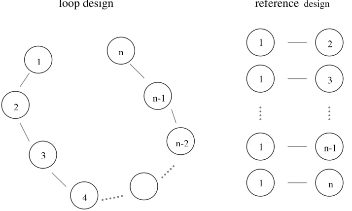
Figure 1. Two common mating designs in plant breeding. For the loop design, candidate parent 1 is cross to 2, 2 to 3, and so on, which results in n-1 families. For reference design, candidate parent 1 is cross to all other parents, which also generates n-1 families.

Each season, plant breeders usually generate many families each with small family size from candidate parents. It is important to investigate how different mating designs among these candidate parents affect QTL analysis. Loop and reference designs are two common mating designs (Figure 1) to generate multiple families in plant breeding. Chapter II explored within-family LD to study the impact of these two mating designs on QTL mapping in multiple families with a Bayesian variable selection approach. Assuming random parents from the germplasm were sampled, the impact of a loop mating design versus a reference mating one on power to detect QTL and to estimate QTL variance and position was studied.

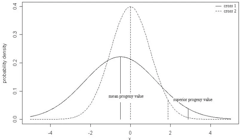
In inbred line development, parents are crossed to generate segregating populations from which superior inbred progeny are selected. The usefulness of a particular cross does not depend on its mean progeny performance but on the performance of its best progeny

(SCHNELL and UTZ, 1975), which was called the superior progeny value here. Plant breeders

1

2

3

4

n

n-1

n-2

loop design reference design

1 ₂

1 3

1 n-1

tend to choose a cross that would have the higher probability of generating better superior inbred lines from a cross (Figure 2). In a typical breeding program, far too many crosses are possible between elite candidate parents for exhaustive evaluation. For example, among 50 elite parents there are 1225 possible crosses. Therefore it would be of great benefit if one could predict, among possible crosses, which ones are most likely to lead to superior inbred lines. Chapter III investigated cross prediction, using QTL analysis results from Bayesian shrinkage analysis that exploits within-family LD from a bi-parental cross. Theory was developed to predict the superior progeny value as a function of the mean of all progeny and of their standard deviation, using QTL analysis results. Different genetic conditions were used to assess the value of the genetic standard deviation in determining the usefulness of a cross.

Chapter IV used barley SNP data to evaluate association-based genomic selection for spring two-row barley, assuming the existence of population-wide LD. We assessed the adequacy of current barley SNP density for genomic selection, and the impact of specific character in plant breeding relative to animal breeding upon genomic selection. The performance of three statistical analyses for genomic selection was compared: random regression best linear unbiased prediction (RR-BLUP) (Meuwissen et al 2001), Bayesian shrinkage estimation from ter Braak et al (2005) and Bayes-B (Meuwissen et al 2001).

Chapter V is general discussions followed by an appendix of the R code for genomic selection.

References

Allard, R.W. 1960 Principles of plant breeding. Wiley, New York.

Arbelbide, M., and R. Bernardo. 2006 Mixed-model QTL mapping for kernel hardness and dough strength in bread wheat. Theoretical and Applied Genetics 112:885-890.

Arbelbide, M., J. Yu, and R. Bernardo. 2006 Power of mixed-model QTL mapping from phenotypic, pedigree and marker data in self-pollinated crops. Theoretical and Applied Genetics 112:876-884.

Beavis, W. D., 1994 The power and deceit of QTL experiments: lessons from comparative QTL studies, p. 250-265, In D. B. Wilkinson, ed. Proceedings of the 49th Annual Corn and Sorghum Research Conference. American Seed Trade Association, Washington, D.C.

Beavis, W. D., 1998 QTL analyses: power, precision, and accuracy, pp. 145-162 in Molecular Dissection of Complex Traits, edited by A. H. PATERSON. CRC Press, New York.

Blanc, G., A. Charcosset, B. Mangin, A. Gallais, and L. Moreau, 2006 Connected populations for detecting quantitative trait loci and testing for epistasis: an application in maize. Theor. Appl. Genet. 113:206-224.

Brahm, L., T. Röcher, and W. Friedt 2000 PCR-Based Markers Facilitating Marker Assisted Selection in Sunflower for Resistance to Downy Mildew. Crop Sci. 40: 676-682.

Breseghello, F., and M.E. Sorrells. 2006 Association mapping of kernel size and quality in wheat (Triticum aestivum L.) cultivars. Genetics 172:1165-1177.

Chen, S., Lin XH, Xu CG, and Zhang Q 2000 Improvement of bacterial blight resistance of Minghui 63, an elite restorer line of hybrid rice, by molecular marker-assisted selection. Crop Science, 40, 239-244.

Dekkers, J. C. M. 2004 Commercial application of marker- and gene-assisted selection in livestock: Strategies and lessons. J. Anim. Sci. 82:E313-E328.

Erlich, H. A., and N. Amheim 1992. Genetic Analysis Using the Polymerase Chain Reaction. Annual Review of Genetics 26: 479-506.

FALCONER, D. S., and T. F. C. MACKAY, 1997 Introduction to Quantitative Genetics.

Longman, New York.

Fehr, W.R., (ed.) 1984 Genetic contributions to yield gains of five major crop plants, pp. 1-101. Crop Science Society of America, Madison, USA.

Fernando, R.L., M. Grossman. 1989 Marker assisted selection using best linear unbiased prediction. Genet. Sel. Evol. 21:467-477.

Flint-Garcia, S.A., J.M. Thornsberry, and E.S. Buckler, IV. 2003 Structure of linkage disequilibrium in plants. Annual Review of Plant Biology. Annual Review of Plant Biology. 54:357-374.

Gianola, D. 2001 Inferences about breeding values, p. 645-672, In D. Balding, et al., eds. Handbook of Statistical Genetics. John Wiley, New York.

Habier, D., R. L. Fernando and J. C. M. Dekkers. 2007 The impact of genetic relationship information on genome-assisted breeding values. Genetics. 177(4):2389-97.

Hoerl, A. E., and R. W. Kennard, 1970 Ridge regression: biased estimation for nonorthogonal problems. Technometrics 12: 55-67.

Hospital, F. and A. Charcosset. 1997 Marker-assisted introgression of quantitative trait loci. Genetics 147:1469-1485.

Jansen, R. C., 1993 Interval mapping of multiple quantitative trait loci. Genetics 135: 205-211.

Joshi, A.K., R. Chand, S. Kumar, and R.P. Singh 2004 Leaf tip necrosis: A phenotypic marker associated with resistance to spot blotch disease in wheat. Crop Sci. 44:792– 796.

Kennedy, B.W., M. Quinton, and J.A.M. vanArendonk.1992 Estimation of effects of single genes on quantitative traits. Journal of Animal Science 70:2000-2012.

Kao C H, Z B Zeng and R D Teasdale 1999 Multiple interval mapping for quantitative trait loci. Genetics 152: 1203-1216.

Lande R, Thompson R 1990 Efficiency of marker-assisted selection in the improvement of quantitative traits. Genetics 124:743-756.

Lewontin, R. C and K. Kojima 1960 The evolutionary dynamics of complex polymorphisms. Evolution 14:458–472.

Lynch M, and B Walsh 1998 Genetics and Analysis of Quantitative Traits. Sinauer Associates, Sunderland, MA.

Luo ZW, Hackett CA, Bradshaw JE, McNicol JW, Milbourne D, 2001 Construction of a genetic linkage map in tetraploid species using molecular markers. Genetics. 157:1369-1385.

Mason SL, Stevens MR, Jellen EN, Bonifacio A, Fairbanks DJ, McCarty RR, Rasmussen AG, Maughan PJ, 2005 Development and Use of Microsatellite Markers for Germplasm Characterization in Quinoa (Chenopodium quinoa Willd.) Crop Science 45:1618-1630.

Meuwissen, T. H. E., B. J. Hayes, and M. E. Goddard, 2001 Prediction of total genetic value using genome-wide dense marker maps. Genetics 157:1819-1829.

Parisseaux, B., and R. Bernardo, 2004 In silico mapping of quantitative trait loci in maize. Theoretical and Applied Genetics 109:508-514.

RebaÔ A, and Goffinet B, 1993 Power of tests for QTL detection using replicated progenies derived from a diallel cross. Theor. Appl. Genet. 86: 1014-1022.

Ritland, K. 2000 Marker-inferred relatedness as a tool for detecting heritability in nature. Molecular Ecology 9:1196-1204.

Satagopan, J. M., B. S. Yandell, M. A. Newton and T. G. Osborn, 1996 A Bayesian approach to detect quantitative trait loci using Markov chain Monte Carlo. Genetics 144: 805-816.

Schon, C. C., H. F. Utz, S. Groh, B. Truberg, S. Openshaw, et al., 2004 Quantitative trait locus mapping based on resampling in a vast maize testcross experiment and its relevance to quantitative genetics for complex traits. Genetics 167:485-498.

Schnell, F.W., and H.F. Utz, 1975 F1-Leistung und Elternwahl Euphy-der Züchtung von Selbstbefruchtern. p. 243–248. Bericht über die Arbeitstagung der Vereinigung österreichischer Pflanzenzüchter. BAL Gumpenstein, Gumpenstein, Austria.

SERVIN,B.,O.C.MARTIN,M.MEZARD, and F.HOSPITAL, 2004 Toward a theory of

marker-assisted gene pyramiding. Genetics 168:513–523.

Sillanpaa M. J., and E. Arjas 1998 Bayesian mapping of multiple quantitative trait loci from incomplete inbred line cross data†Genetics 148 (3): 1373-1388.

Singh S., Sidhu J. S., Huang N., Vikal Y., Li Z., Brar D. S., Dhaliwal H, Khush G. S. 2001 Pyramiding three bacterial blight resistance genes (xa-5, xa-13 and Xa21) using marker-assisted selection into indica rice cultivar PR106. Theor. Appl. Genet. 102:1011-1015.

Smith J. S. C., S. Kresovich, M.S. Hopkins, S.E. Mitchell, R.E. Dean, W.L. Woodman, M. Lee, and K. Porter, 2000 Genetic Diversity among Elite Sorghum Inbred Lines Assessed with Simple Sequence Repeats. Crop Sci. 40: 226-232.

Thornsberry, J. M., M. M. Goodman, J. Doebley, S. Kresovich, D. Nielsen, and E. S. Buckler. 2001 Dwarf8 polymorphisms associate with variation in flowering time. Nature Genetics 28:286-289.

Verhoeven, K. J. F., J.-L. Jannink, and L. M. McIntyre, 2006 Using mating designs to uncover QTL and the genetic architecture of complex traits. Heredity 96:139-149. Wang, G., T. S. Whittam, C. M. Berg, and D. E. Berg. 1993 RAPD (arbitrary primer) PCR is

more sensitive than multilocus enzyme electrophoresis for distinguishing related bacterial strains. Nucleic Acids Res. 21:5930-5933.

Wang, H., Y. M. Zhang, X. M. Li, G. L. Masinde, S. Mohan, et al., 2005 Bayesian shrinkage estimation of quantitative trait loci parameters. Genetics 170:465-480.

Weeden, NF, and JF Wendel. 1990 "Genetics of plant isozymes". Pp. 46-72 in D. E. Soltis and P. S. Soltis, eds. Isozymes in plant biology. Chapman and Hall, London.

Whittaker, J. C., R. Thompson, and M. C. Denham, 2000 Marker-assisted selection using ridge regression. Genetical Research 75:249-252.

Willcox, M. C., M. M. Khairallah, D. Bergvinson, J. Crossa, J. A. Deutsch, et al 2002 Selection for resistance to southwestern corn borer using marker-assisted and conventional backcrossing. Crop Sci. 42: 1516-1528.

Winter P, and G. Kahl 1995 Molecular marker technologies for crop improvement. World J Microbiol Biotechnol 11:449-460.

Xie, C. Q., D. D. G. Gessler and S. Z. Xu, 1998 Combining different line crosses for mapping quantitative trait loci using the identical by descent-based variance component method. Genetics 149: 1139-1146.

Xu, S., 1998 Mapping quantitative trait loci using multiple families of line crosses. Genetics 148: 517-524.

Xu, S., 2003a Theoretical Basis of the Beavis Effect. Genetics 165:2259-2268.

Xu, S., 2003b Estimating polygenic effects using markers of the entire genome. Genetics 163:789-801.

Yu, J., G. Pressoir, W.H. Briggs, I. Vroh Bi, M. Yamasaki, J.F. Doebley, M.D. McMullen, B.S. Gaut, D.M. Nielsen, J.B. Holland, S. Kresovich, and E.S. Buckler, IV. 2006 A unified mixed-model method for association relatedness. Nat. Genet. 38:203-208. Yu J, Holland J B, M D McMullen, and E S. Buckler 2008 Genetic Design and Statistical

Power of Nested Association Mapping in Maize. Genetics 178: 539-551.

Zabeau, M and P. Vos. 1993 Selective restriction fragment amplification: a general method for DNA fingerprinting. European Patent Office, publication 0 534 858 A1, bulletin 93/13.

CHAPTER II. COMPARISON OF TWO MATING DESIGNS

FOR MULTIPLE-FAMILY QTL MAPPING

A paper to be submitted to Crop Science

Shengqiang Zhong and Jean-Luc Jannink

Abstract

Multiple-population quantitative trait locus (QTL) mapping integrates and uses information from many populations, and may improve QTL mapping and QTL-based breeding programs. Mating designs that maximize the value of multiple-population analysis have not been studied. Here, we simulated populations from two divergent designs, a reference design in which all parents are crossed to a reference parent, and a loop design in which parents are randomly ordered and crossed in a chain. Each design generated 12 families of 50 F2 progeny. The genome consisted of seven 140 cM chromosomes, each

carrying one QTL. The total QTL heritability was 0.42. The relative QTL detection power of the loop and reference designs depended on the detection threshold adopted. For typical thresholds (with an average detection power of 0.35) the loop design was most powerful, while for more stringent thresholds the reference design was most powerful. In all cases, the loop design gave more accurate estimates of QTL position and effect size. In general, we would recommend the loop design over the reference design for multiple-population QTL mapping.

Introduction

Characterizing the genetic architecture of a population requires detecting QTL and estimating the variance they generate. Traditional QTL mapping methods developed for progenies from a cross between two inbred parents have the problem of poor generalizability of the findings (Muranty, 1996; Xu, 1998). Comparisons of QTL mapping results from different populations suggest that, despite of some consensus QTL intervals across different mapping populations, a considerable amount of the QTL effects are family-specific (Welz and Geiger 2000; Kolb et al 2001; Kamoshita et al 2002; Clancy et al 2003; Chardon et al. 2004). Multiple-family QTL mapping, first proposed by Muranty (1996), can avoid this problem. Studies have shown that using multiple line crosses broadens the parameter inference space to the reference population, leads to more generalizable inferences about QTL, and can increase QTL detection power (Muranty, 1996; Xu, 1998; Rebaï and Goffinet, 2000; Jannink, 2001).

Important theoretical developments have been made on QTL detection methods in interconnected families. Statistical methods can be distinguished into three categories: regression analyses (Rebaï and Goffinet 2000), maximum-likelihood methods (Liu and Zeng, 2000), and Bayesian approaches (Xu, 1998; Jannink and Wu, 2003). Bayesian methods have been demonstrated to be able to accommodate more complicated models, such as variable QTL number (Satagopan, 1996; Sillanpaa, 1998; Xu, 1998) and variable allele configuration models (Jannink and Wu, 2003). In these analyses, QTL allele effects have been considered fixed (Rebaï and Goffinet, 1993; Rebaï et al., 1994; 2000; Liu and Zeng, 2000) or random (Xu, 1998; Xie et al., 1998; Jannink and Wu, 2003). Fixed allele effect models relax the assumption of normally distributed allele effects but face the problem of estimating a large number of parameters when many families are analyzed jointly and all parental alleles are assumed to have distinct effects. Random allele effect models estimate only a single allelic effect variance, so the number of parameters per QTL is independent of the number of families.

of relevant parameters are needed. Researchers have investigated how different sampling strategies (family number vs. family size) might affect QTL detection power (Xie et al 1998; Xu 1998; Rao and Li 2000) and QTL allelic number and variance estimation (Wu and Jannink 2004). These studies showed that the power of QTL detection was higher with an intermediate number of families than with a small number of large families or a large number of small families. As to the effect of mating design on QTL mapping, Muranty (1996) showed that when the number of families and the number of offspring per family were held constant, QTL detection power was affected by the number of outbred parents used in the design but the arrangement of the outbred parents in specific diallel designs had little impact. Wu and Jannink (2004) investigated a circulant diallel mating design. This design is sometimes used in plant breeding practice (e.g., DeKoeyer and Stuthman, 1998) and would therefore be a logical choice for combining QTL analyses with further advancing a breeding program. For the specific purpose of distinguishing among QTL alleles carried by different parents, however, they pointed out that the circulant diallel design may not be the most effective crossing scheme. Alleles carried by two parents will be contrasted with the greatest power if those two parents are crossed directly. This reasoning suggests that all pair-wise crosses be performed among parents sampled from the reference population, leading to a half-diallel design. Verhoeven et al. (2006) explored QTL detection power with a fixed number of parents under different mating designs. For a fixed experiment size, they found that QTL detection power was greatest for the mating design with the fewest but largest families (circulant diallel mating design) while power was lowest for the design with the most, smallest families (the half diallel). This study showed that half-diallel design analyzing a high number of families was not the best. Another alternative is to cross all sampled parents to the same reference parent. This approach does not allow the direct contrasts among QTL alleles that the half-diallel allows, but instead an indirect contrast relative to a very-well characterized reference allele.

assumes that a fixed number of individuals have been randomly picked from a base population and inbred to homozygosity to be used as parents in the mating designs. These homozygous parents are then crossed to generate F2 QTL mapping families of a fixed size.

Methods

Simulations

(i) Mapping families: The mapping families were generated using either a modified loop design or a reference design. In the loop design, inbred founders were randomly ordered and each founder was mated with its immediate neighbors in the list. The first and the last parents on the list were mated once, while all other parents were mated twice. In the reference design, a single inbred founder was chosen at random to be the reference parent, and all other founders were crossed to it. Both designs generate P – 1 families from P founding inbred

parents. Here, 13 inbred founders were used to generate 12 F2 mapping families, with 50 F2

progenies in each family leading to a fixed experimental size of 600.

(ii) Genome, markers and QTL: The simulated genome consisted of 7 chromosomes of a length of 140 cM for a total genome size similar to barley. The marker spacing was 10 cM, markers were co-dominant and informative in all crosses. Seven additive effect QTL were simulated on the genome with one QTL on each chromosome. As in Verhoeven et al. (2006), each inbred founder was simulated to carry a unique QTL allele. The effects of these QTL in terms of the additive variance contributed to the trait varied in a geometric series (Lande and Thompson, 1990). The percent of the phenotypic variance generated by the QTL in the random-mating F2 population were 12, 9, 7, 5, 4, 3, and 2 for a total heritability of 0.42. All

QTL were simulated at 45 cM from the end of their chromosome.

QTL model and statistical analysis

(i) QTL model Consider a simple additive model for F2 populations, where the trait of

interest is affected by J QTL. Let N be the total number of F2 progeny that were produced by

K F1 individuals, and the latter were derived from P inbred founders. Assume that each

y=Xβ+ Q_jα_j

j=1 J

∑ +ε (1)

whereX is an N×K design matrix relating an F2 progeny to the F1 family from which it is

derived, β is a K×1 vector of family means, Qj is a N×P matrix relating a progeny to the

allele that QTL j carries, αj is a P×1 vector of allelic effects at QTL j, and ε ~ N(0, Iσ

2_{) is a}

N× 1 vector of residuals.

(ii) Statistical model We observe trait values (y), family structure (X) and marker

genotypes (M). Marker genotypes are considered fixed and the analysis is conditioned on the marker genotypes observed. We wish to infer the number of QTL (J), QTL positions (Λj),

QTL genotypes of each progeny (Q_j), allelic effect variance for each QTL (σ2_j), allelic

effects (αj), family means (β), and residual variance (σ

2_{). We employ a Bayesian analysis}

with the following priors. The prior for J is Poisson with mean λ, the expected QTL number

in the genome. The prior for Λj is uniform over the genome so that p(Λj) = (genome size)

-1_.

The prior for Qj follows the rules of Mendelian segregation and recombination conditioned

on Λj and on flanking markers. Allelic effects are treated as random, where the prior for αj is normal with mean zero and variance σj

2_{. σ} j

2 _{is considered a random variable to be estimated}

with uniform prior distribution σj 2 _~

unif(0,σ_max2 ), where σ_max2 is a maximum value that we

believe allelic effect variance can take. Denote θ =(β,σ2_,{Λ

j}j=1 J _,{

Q_j}J_j=1,{α_j}J_j=1,{σ2_j}J_j=1) the vector of all unobservable

parameters, excluding the number of QTL. The joint posterior density of all unobservable parameters (J,θ) given the observable (y,X,M) and prior information is

p(J,θ|y,X)∝p(y|θ,J)p(J)p(β)p(σ2)p(Λ) p(Q_j |Λ,M)

j=1 J

∏ _p(α

j |σj 2₎ j=1

J

∏ _p(σ

j 2_{) (2)}

where p(y|J,θ) represents the likelihood assuming ε ~ N(0, Iσ2) and p(*) is the prior

distribution for parameter *, with p(Q_j |Λ,M) being the prior distribution for genotypes at

QTL j conditional on QTL positions and flanking markers genotypes, p(αj |σj

2_{)being the}

normal prior distribution for allele effects conditional on allelic effect variance, and p(J)

(iii) Model implementation by Markov chain Monte Carlo (MCMC). The analysis was

accomplished by repeatedly sampling from the posterior distribution using Markov chain Monte Carlo techniques. Parameter estimates were then provided by their marginal posterior distributions. We employed a scalar Metropolis-Hastings algorithm where each parameter in

θ was sampled in turn, considering all other parameters fixed (Gilks et al., 1996). The exception to this scalar implementation was that when updating QTL position, QTL genotypes, allelic variance and allelic effects were sampled jointly with the position. Note that the dimension of the parameter vector θ changes when the number of QTL J is changed.

We thus used a reversible jump Metropolis-Hastings step to move between different numbers of QTL by either adding a new QTL to the model or dropping an existing QTL from the model (Jannink and Fernando, 2004).

After all parameters were initialized from their priors, a complete MCMC iteration consisted of the following steps:

• Update QTL allele effects αj for each QTL j and each inbred founder P

• Update QTL position: update position Λj and genotypes Qj, allelic effect variance σj 2_,

and allele effects αj jointly for each QTL j

• Update family means β, and residual variance σ2

• Update the number of QTL J

For a given number of QTL, the steps for updating QTL allele effects, position, family means, and residual variance were described in detail in Wu and Jannink (2004). The methods of updating the number of QTL under a random allele effect model were adapted from Jannink and Fernando (2004).

QTL detection power, allelic variance and position estimation

Location-wise QTL intensity was defined in 1 cM bins as the probability that a QTL was sampled in that bin over the 120,000 samples. Sliding windows of 10 cM over which intensity was integrated were used to evaluate QTL detection power, accuracy of map position estimation, and location-wise QTL variance. Integrated intensity and average QTL variance centered at two kinds of positions were obtained. One was the true QTL position (pos_True). The other was obtained by identifying the 10 cM window where integrated

intensity was maximized (pos_max). The summary statistic pos_max was also used as an

estimator of QTL position. An additional estimator of QTL position was the expected posterior QTL position (Epos) for each chromosome, as follows. Assuming chromosome

length chrL,

∑

∑

, where intensityi was the location-wise intensity at bin

i.

We determined the statistical power for detecting a QTL by counting the number of runs where the 10 cM integrated intensity surrounding the true position was greater than a certain threshold, or by counting the number of runs where the integrated intensity surrounding

max

pos was greater than a certain threshold and pos_maxwas within 10 cM of the true position.

Let π₀ be the prior QTL intensity. In the present analysis, π₀=J [QTL]/9.8 [Morgans],

where J is the average number of QTL (parameter J above) over MCMC iterations, and 9.8

is the simulated genome size in Morgans. For the FM model, J =7 and π₀=7 [QTL]/9.8

[Morgans]=0.714 [QTL/Morgan]; for the VM model, J needed to be calculated for each

To quantify the accuracy of QTL allelic variance and position estimation, the mean

squared error (MSE), (_θˆ) 2(_θˆ) (_θˆ) Var Bias

MSE = + , the sum of the squared measurement

bias and the measurement variance were used. Measurement variance was the usual variance

among replicate estimates. Bias was calculated as θ

∑

( where R was the

number of replicate simulations, θˆ_r was the estimate in simulation r, and θ was the true

value. Two kinds of QTL allelic variance estimator was obtained as the average QTL

variance at pos_True and pos_max. Two kinds of estimators, pos_max and Epos, were utilized to

estimate QTL position..

Results

QTL number in reversible jump MCMC

The average QTL numbers of VM model were 5.30±0.07 and 5.86±0.07 in the reference and loop design, respectively. These estimates were smaller than the true QTL number (7), possibly due to the small allelic variance of some QTL in the genome. Nevertheless, the VM model selected a number of QTL closer to the true number when analyzing the loop design than when analyzing the reference design, indicating that the loop design was better than the reference design from this perspective.

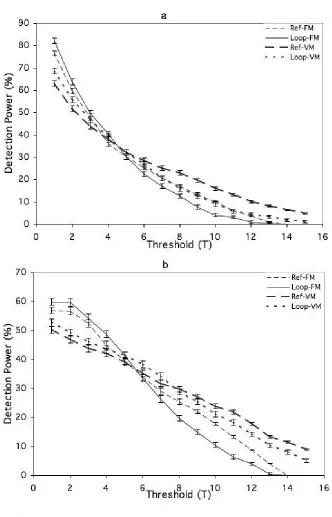
QTL detection power

Using a 3T threshold, detection power from pos_True was 4% and 6% higher for the loop

design than for the reference design, under the FM and VM models, respectively (Figure 1a);

detection power from pos_maxwas similar for two mating designs under the FM model but 5%

higher for the loop design under the VM model (Figure 1b). Interestingly, as the threshold that was used to declare detection increased and the detection power decreased, the reference design increased in power relative to the loop design, such that for high thresholds (> 7T), the

reference design was more powerful than the loop design for both the FM and the VM model (Figure 1a and 1b).

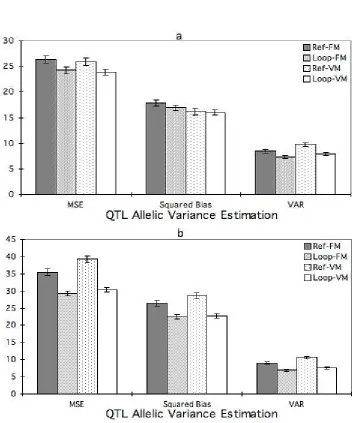
QTL allelic variance

design (Figure 2a and 2b). The MSE fromposTrue, was 8% lower for the loop than the

reference design under both FM and VM. The MSE from pos_max, was 17% lower for the loop

design than for the reference design under FM, and 23% under VM.

QTL position

The MSE for QTL position was smaller for the loop than the reference design for both

FM and VM and for both position estimates, Epos and pos_max (Figure 3a and b). The MSE

using Epos was 5% lower for the loop design than for the reference design under FM, and

9% under VM. The MSE using pos_maxwas 6% lower for the loop design than for the

reference one under FM, and 11% under VM.

Discussion

Joint analysis of multiple families, first introduced by Muranty (1996), extends QTL mapping to a broader inference space with respect to the reference population and can reduce the problem of non-segregating QTL in single cross (Xu, 1998). Thus multiple-family QTL mapping can improve QTL detection at the population level and be incorporated into practical breeding programs for individual genotypic value prediction (Verhoeven et al, 2006).

rest to just one family. It is interested to investigate other intermediate situations.

Although the reference design offers a well-characterized reference allele with which to contrast the other alleles and might therefore increase QTL detection efficiency (Wu and Jannink 2004), the results presented here suggest that it causes insufficient representation of the other alleles, which naturally generates larger variance for parameter estimation from experiment design view. This reduced representation appears to reduce the efficiency of the analysis from several perspectives. In particular, simulations showed that the loop design estimated QTL position and QTL variance with lower mean squared error than the reference design. Both designs detected QTL with similar power over different thresholds, but the loop design showed higher power when lower detection thresholds were adopted while the reference design showed higher power when higher detection thresholds were adopted.

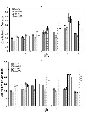
To understand this phenomenon, we analyzed the mean and coefficient of variation (CV)

of the 10 cM integrated intensity either from posTrue or from posmax. The mean integrated

intensity of QTL was similar for the loop and reference designs (Figure 4a and b). Mixed

model analysis showed that design had no overall effect on integrated intensity from posTrue

(P = 0.421), but integrated intensity from pos_max in the reference was 4% higher than in the

loop design (P = 0.046). The CV of the integrated intensity was consistently larger in the reference design than in the loop design (Figure 5a and b). Analysis of the residual variances from the mixed models (Littell and Ramon, 1996) showed that the residual variance in the reference design was larger than that in the loop design for integrated intensity from both

True

pos (P < 0.001) and pos_max(P < 0.001).

reference design, it would be preferred to select a reference parent with high or low breeding value for single trait QTL mapping, although it might not be easy to select such a reference parent for QTL mapping in multiple traits.

In conclusion, because the loop design more uniformly represents alleles sampled from a base population it offers advantages over the reference design in terms of characterizing QTL. In the present study, these advantages were small but detectable: the loop design gave more accurate estimates of the QTL position and of the variance generated by the QTL. For QTL detection power, the results were somewhat more equivocal. Nevertheless, we would recommend the loop design over the reference design because low CV of QTL intensity, as given by the loop design, will result in more consistent QTL detection performance.

References

Blanc G, Charcosset A, Mangin B, Gallais A, Moreau L (2006) Connected populations for detecting quantitative trait loci and testing for epistasis: an application in maize Theor Appl Genet 113:206–224.

Chardon F, Virlon B, Moreau L, Falque M, Joets J, Decousset L, et al. (2003). Comparative mapping of beta-amylase activity QTLs among three barley crosses. Crop. Sci. 43: 1043-1052.

De Koeyer, DL, and D.D. Stuthman (1998). Continued response through seven cycles of recurrent selection for grain yield in oat (Avena sativa L.). Euphytica 104:67-72.

Gilks WR, Richardson S, Spiegelhalter DJ (1996) Introducing Markov chain Monte Carlo. In: Gilks WR, Richardson S, Spiegelhalter, DJ (eds) Markov chain Monte Carlo in practice. Chapman and Hall, London, pp 1–19.

Jannink JL, Fernando RL (2004). On the Metropolis-Hastings acceptance probability to add or drop a quantitative trait locus in Markov chain Monte Carlo-based Bayesian analyses. Genetics 166: 641–643.

Jannink JL, Wu XL (2003). Estimating allelic number and identity in state of QTLs in interconnected families. Genet Res 81: 133–144.

Kamoshita A, Wade LJ, Ali ML, Pathan MS, Zhang J, Sarkarung S et al (2002). Mapping QTLs for root morphology of a rice population adapted to rainfed lowland conditions. Theor. Appl. Genet. 104: 880-893.

Kolb FL, Bai GH, Muehlbauer GJ, Anderson JA, Smith KP, Fedak G (2001). Host plant resistance genes for fusarium head blight: Mapping and manipulation with molecular markers. Crop. Sci. 41: 611-619.

Lande R, Thompson R (1990). Efficiency of marker-assisted selection in the improvement of quantitative traits. Genetics 124:743-756.

Littell, Ramon C. SAS system for mixed models. Cary, N.C. : SAS Institute, Inc., c 1996. Liu YF, Zeng ZB (2000). A general mixture model approach for mapping quantitative trait

loci from diverse cross designs involving multiple inbred lines. Genet. Res. 75: 345-355.

Muranty H (1996). Power of tests for quantitative trait loci detection using full-sib families in different schemes. Heredity 76: 156-165.

Rao SQ, Li X (2000). Strategies for genetic mapping of categorical traits. Genetica 109: 183-197.

Rebaï A, Goffinet B (2000). More about quantitative trait locus mapping with diallel designs. Genet. Res. 75: 243-247.

Rebaï A, Goffinet B, Mangin B, Perret D (1994) Detecting QTLs with diallel schemes. In van Ooijen JW, Jansen J (eds) Biometrics in Plant Breeding: Applications of Molecular Markers, 9th meeting of the EUCARPIA, Wageningen, the Netherlands, CPRO-DLO, pp. 170-177.

Satagopan JM, Yandell YS, Newton MA, Osborn TC (1996). A Bayesian approach to detect quantitative trait loci using Markov chain Monte Carlo. Genetics 144: 805-816.

Sillanpaa MJ, Arjas E (1998) Bayesian mapping of multiple quantitative trait loci from incomplete inbred line cross data. Genetics 148:1373-1388.

Welz HG, Geiger HH (2000). Genes for resistance to northern corn leaf blight in diverse maize populations. Plant Breeding 119: 1-14.

Wu XL, Jannink JL (2004). Optimal sampling of a population to determine QTL location, variance, and allelic number. Theor. Appl. Genet. 108: 1434-1442.

Xie C, Gessler DD, Xu S (1998) Combining different line crosses for mapping quantitative trait loci using the identical by descent-based variance component method. Genetics 149:1139-1146.

Figures

Figure 1. QTL detection power under different thresholds for the reference (Ref) and Loop

designs for models with fixed (FM) or variable (VM) numbers of QTL fitted. The results were from 200 replicate simulations and the error bars are standard error. Power was estimated using 10 cM integrated intensity averaged over the seven simulated QTL at their a. true position , and b. estimated QTL position.

Figure 2. Mean square error (MSE), squared bias and measurement variance (VAR) of posterior QTL allelic variance for the reference (Ref) and Loop designs for models with fixed (FM) or variable (VM) numbers of QTL fitted. The above three statistics (MSE, Squared Bias and Var) were averaged over the seven simulated QTL at their a. true position, and b. estimated QTL position. Each standard error bar in the graph represents an average of each statistic over all seven QTL and all replicate simulations.

Figure 3. Mean square error, squared bias and measurement variance of QTL position estimation for the reference (Ref) and Loop designs for models with fixed (FM) or variable (VM) numbers of QTL fitted. The above three statistics (MSE, Squared Bias and Var) were averaged over the seven simulated QTL at their a. estimated expected QTL position Epos,

and b. another estimated QTL position pos_max. Each standard error bar in the graph

represents an average of each statistic over all seven QTL and all replicate simulations.

Figure 4. Average 10 cM integrated intensity at the a. expected QTL position Epos, and b.

another estimated QTL position pos_max across 200 replicate simulations for the reference

(Ref) and Loop designs for models with fixed (FM) or variable (VM) numbers of QTL fitted. QTL allelic variance simulated became smaller from QTL 1 to QTL.

Figure 5. Coefficient of variation of 10 cM integrated intensity at their a. estimated expected

QTL position Epos, and b. another estimated QTL position pos_max across 200 replicate

CHAPTER III. USING QTL RESULTS TO DISCRIMINATE AMONG

CROSSES BASED ON THEIR PROGENY MEAN AND VARIANCE

Published in Genetics

Shengqiang Zhong* and Jean-Luc Jannink†1

Abstract

In order to develop inbred lines, parents are crossed to generate segregating populations from which superior inbred progeny are selected. The value of a particular cross thus depends on the expected performance of its best progeny, which we call the superior progeny value. Superior progeny value is a linear combination of the mean of the cross’s progeny and their standard deviation. In this study we specify theory to predict a cross’s progeny standard deviation from QTL results and explore analytically and by simulation the variance of that standard deviation under different genetic models. We then study the impact of different QTL analysis methods on the prediction accuracy of a cross’s superior progeny value. We show that including all markers, rather than only markers with significant effects, improves the prediction. Methods that account for the uncertainty of the QTL analysis by integrating over the posterior distributions of effect estimates also produce better predictions than methods that retain only point estimates from the QTL analysis. The utility of including estimates of a cross’s among-progeny standard deviation in the prediction increases with increasing heritability and marker density but decreasing genome size and QTL number. This

* _{Department of Agronomy, Iowa State University, Ames, Iowa 50011-1010,} †_{USDA–ARS, U.S. Plant, Soil,}

and Nutrition Laboratory, Ithaca, New York 14583 Running head: Selection among crosses

Keywords: Genome-wide selection, Marker assisted selection, Progeny variance, Prediction accuracy, QTL analysis

1

Corresponding author: Jean-Luc Jannink, USDA–ARS, U.S. Plant, Soil, and Nutrition Laboratory, Ithaca,

New York 14583 Phone: (607)-255-5266. Fax: (607)-255-6683.

utility is also higher if crosses are only envisioned among the best parents rather than among all parents. Nevertheless, we show that among crosses the variance of progeny means is generally much greater than the variance of progeny standard deviations, restricting the utility of estimates of progeny standard deviations to a relatively small parameter space.

INTRODUCTION

In inbred line development, parents are crossed to generate segregating populations from which superior inbred progeny are selected. The value of a particular cross depends on the performance of its best progeny rather than on its mean progeny performance. In a typical breeding program, far too many crosses are possible between elite candidate parents for exhaustive evaluation. For example, among 50 elite parents there are 1225 possible crosses. Even if it were feasible to evaluate a sufficient set of progeny from all those crosses, it is unlikely that that would be efficient. Rather, one would want to predict, among possible crosses, which ones are most likely to lead to superior inbred lines.

SCHNELL and UTZ (1975) introduced the usefulness concept for line development. Their

definition of the usefulness of the cross m was: Um =µm+ ∆Gm =µm+iσG(m)hm, where µm is the population mean of homozygous lines that can be derive from cross m, σG(m)

2 _{is the}

genetic variance among these lines, hm is the square root of the heritability, and i is the standardized selection intensity. Two other criteria to similar usefulness are the varietal ability (WRIGHT, 1974; GALLAIS, 1979), and the probability of obtaining transgressive

segregants (JINKS and POONI, 1976). Here, rather than focus on the genetic gain that might be

obtained within a cross, we sought a simpler characterization that would express which crosses would generate progeny with higher genotypic values. Given the focus on genotypic value, we ignored the heritability to obtain what we call the superior progeny value,

s_m=µ_m+iσ_G(m). With this definition, sm equates to Um with a heritability of 1.

In traditional breeding based solely on phenotypic measurements, µm can be predicted

from the breeding values of the two parents but the only information available relevant to

predicting σG(m)