Development of a baited video technique and spatial models to explain patterns of fish biodiversity in inter-reef waters

Full text

(1)This file is part of the following reference:. Cappo, Mike (2010) Development of a baited video technique and spatial models to explain patterns of fish biodiversity in inter-reef waters. PhD thesis, James Cook University. Access to this file is available from: http://eprints.jcu.edu.au/15420.

(2) 6.. SHELF-SCALE PATTERNS OF VERTEBRATE ASSEMBLAGES IN THE INTER-REEFAL WATERS OF THE GREAT BARRIER REEF MARINE PARK. 6.1. INTRODUCTION. Definition of environmental boundaries in species ranges, species assemblages and species ‘stock structure’ is central to conservation planning, fisheries management and the understanding of ecosystem and evolutionary processes. This is particularly important in the tropics, where marine fisheries exploit co-occurring vertebrates in large assemblages (hundreds of taxa) of ‘target’ and ‘bycatch’ species (Sainsbury et al. 1997). For the purposes of this thesis, an assemblage is defined as the species available (to the BRUVS sampling technique) in the same place at the same time. Ecological analysis of assemblage structure can assist in defining spatial ‘assemblage production units’ for the assignment of particular zones of a fishery to specific sectors, gear types and harvest pressures (Garces et al. 2006b). Such analysis can also be used with knowledge of spatial patterns in fishing effort and vulnerability to capture to assess risks to metapopulations exposed to locally intensive fishing pressure (Pitcher et al. 2000; Astles et al. 2006; Ellis et al. 2008). If the relationship between assemblages and critical features of their habitats (such as substratum type) is known well, then ‘area-based management’ could use maps of major habitat features as a proxy for the populations themselves (Bax & Williams 2001; Anderson et al. 2005; Anderson & Yoklavich 2007; Haywood et al. 2008; Anderson et al. 2009). Marine protected areas (MPAs) are now using these surrogates to complement management of fisheries and tourism or to conserve marine biodiversity and marine resources for their intrinsic values (Agardy et al. 2003; Babcock 2003; Faith et al. 2004; Ashworth & Ormond 2005; Evans et al. 2008). These trends towards managing areas rather than single species imply that robust models must be developed to explicitly link biotic and abiotic characteristics of shelf habitats to the distribution of both exploited and unexploited species in assemblages (Ward et al. 1999). However, a major lack of fishery-independent information has prevailed in almost all tropical shelf provinces (see Garces et al. 2006a and Stobutzki et al. 2006b for review). Research trawls, often aimed at discovering potential for fishery development, have provided the only historic data sources for ecological analysis of species assemblages (Koranteng 2001; Joanny & Menard 2002; Le Loeuff & Zabi 2002). Despite the fact that Asia alone supplies nearly sixty percent of global fish production, only recently has a standardised, georeferenced database on trawl catches become available for the shelves in that region (Pauly & Chuenpagdee 2003; Garces et 143.

(3) al. 2006a). Only depth and position was routinely recorded at these trawl stations, so the underlying causes of spatial patterns have not been examined. Whilst cross-shelf zonations in fish assemblages attributed to depth have been a feature of the tropical shelf studies (García et al. 1998; Koranteng 2001; Garces et al. 2006b), a great variety of other known (or unknown) environmental covariates are collinear with depth (Murawski & Finn 1988; Mahon & Smith 1989). Studies of the bycatch from prawn trawl fisheries have provided additional information on broad-scale geographic patterns, but without supporting data on the habitats trawled it has been difficult to interpret their findings (Ramm et al. 1990; Tonks et al. 2008). Relatively few measurements of temperature, salinity, and sediment particle size and composition have been made in conjunction with tropical trawl surveys (Harris & Poiner 1991; Blaber et al. 1994; Pierce & Mahmoudi 2001; Haywood et al. 2008), and direct measurement and characterisation of the epibenthic communities in the path of these trawls has been even rarer (Sainsbury et al. 1992; Sainsbury et al. 1997). Thus hydrology and characteristics of the substratum were often inferred from other studies to interpret spatial patterns in trawl catches (Bianchi 1992b; 1992a; Bianchi et al. 2000). In combination these factors have hampered multivariate analyses of the relationships between tropical species and their environments. The earliest work by Fager & Longhurst (1968) and Lowe-McConnell (1987) in West Africa produced persistent generalisations that fish communities were influenced most by latitude, hydrology, depth and sediment coarseness. These authors confidently characterised tropical shelves everywhere by cross-shelf gradients from muddy coastal waters, dominated by riverine inputs, to sand and sponge gardens amongst ‘rock and dead coral’ under influences of oceanic currents. They proposed abrupt changes in the distribution of fish families comprising communities along that gradient. Inshore ‘brown water’ communities were reported to be dominated by ariid catfishes and dasyatid rays over mud, shifting to a ‘golden fish’ zone dominated by sciaenid croakers over sandy/mud. Further offshore, in ‘green water’ (40-60 metres deep), a ‘silver fish’ zone of carangid jacks and haemulid grunts was proposed to reside above a ‘red fish’ zone of lutjanid snappers over hard sand and rock in ‘blue’ oceanic waters around one hundred metres deep. The cooler waters below permanent or seasonal thermoclines were characterised by the presence of a ‘sparid’ assemblage. These simple generalisations remain in the literature to this day, implying wide determinism at provincial scales in the dominance of sciaenids, ariids, sparids, haemulids and lutjanids in tropical assemblages depending upon depth, temperature and the nature of underlying sedimentary deposits (Longhurst & Pauly 1987; Longhurst 2007).. 144.

(4) The ‘soft-bottom’ plains between the reefs of the GBRMP, and in the large lagoons of atoll islands such as New Caledonia, also support major fisheries for prawns or finfish. They are comprised largely of shallow, sheltered, well-mixed lagoons behind a shelf-edge barrier of coral reefs, and the roles of upwelling and thermoclines highlighted by Longhurst & Pauly (1987), Le Loeuff & Zabi (2002) and Longhurst (2007) are of less relevance than the presence of biogenic structures, riverine inputs and tidal forcing. Nevertheless, a variety of strong gradients in these lagoons have measurable influences on the vertebrate fauna (Williams & Hatcher 1983; Russ 1984; Newman et al. 1997; Letourneur et al. 1998; Letourneur et al. 1999; Kulbicki et al. 2000; Gust et al. 2001; Begg et al. 2005; Burridge et al. 2006; Beger & Possingham 2008; Hoey & Bellwood 2008; Wismer et al. 2009). The shelf-scale patterns in species richness I described in Chapter 5 fitted well with general expectations based on knowledge of gradients and boundaries in sedimentary processes, water movement and seafloor fish habitats. The position along and across the shelf were shown to be very useful surrogates for major hydrological and sedimentary variables suspected to constrain the distribution and abundance of marine vertebrates. The position of sites within the GBRMP has also recently been assessed as a surrogate for measurements of chlorophyll, phaeophtyin, nitrate and turbidity (Fabricius & De’ath 2001a; 2001b; 2004; Devlin & Brodie 2005; Fabricius et al. 2005; Fabricius 2005; Brodie et al. 2007; Fabricius & De’ath 2008; Fabricius et al. 2008). In turn, these environmental drivers have repeatedly been used to explain the distributions of autotrophs and heterotrophs (Carruthers et al. 2002; Fabricius et al. 2005; DeVantier et al. 2006; Fabricius & De’ath 2008), and predict the effects of changes in water quality at the scale of the entire GBRMP (Carruthers et al. 2002; Brodie 2003; Fabricius et al. 2005; DeVantier et al. 2006; Wooldridge et al. 2006; Fabricius & De’ath 2008; Brodie & Fabricius 2009). It might be argued that the dimensionless positions ‘across’ and ‘along’ were unique to the GBRMP shelf and therefore not directly transportable to other shelf systems, such as the Torres Strait or the large lagoons of New Caledonia. Identification of the major environmental correlates underlying the spatial surrogates is therefore desirable to allow both a better definition and interpretation of vertebrate assemblages in terms of seafloor habitats, and for better contrasts to be made with assemblages in other Indo-Pacific regions. In this chapter I attempt to determine if environmental mechanisms, thresholds and interactions can be identified to improve predictions and explanations of shelf-scale patterns in assemblages. To do this I use multivariate analyses of vertebrate assemblage structure with nineteen of the top environmental predictors of species richness distinguished in Chapter 5. I use multivariate regression trees (De’ath 1999; 2002) and Dufrêne-Legendre indices to define spatially 145.

(5) contiguous vertebrate assemblages of fishes, sharks, rays and seasnakes, constrained by the spatial and environmental values that locate them in the GBRMP. At each node in the tree I examine the improvements in the model predictions provided by the primary splitting variable and also the alternative, surrogate splitting variables. This will provide insights into the influence of underlying environmental covariates that were collinear with the position and depth of sites on the GBRMP shelf. 6.2. METHODS. The survey design, 366 BRUVS sites and environmental covariates have been described in detail in Chapter 5.2. In this chapter I used only the nineteen most complete, and most influential, environmental covariates distinguished in Chapter 5.2.3.2. These covariates were percentage composition of sediments (coarsns.pc, carbnte.pc, gravl.pc, sand.pc, mud.pc), position (across, along), depth, interpolated seabed current shear stress and hydrology (Current, Salin.av, Salin.sd, Temp.av, Temp.sd), and analyses of the seafloor footage obtained by video tows. These were measures of location and spread of substratum complexity (rugosity.vid.av, rugosity.vid.sprd), the percentage of the video track comprised of bare or bioturbated seabed (bare.pc.vid, biotrb.pc.vid), and the percentage of the track comprised of marine plants or megabenthos (plant.pc.vid, mgbnths.pc.vid). The towed video data (with the ‘vid’ suffix) were used because they were more comprehensive (342 sites) than the analysis of still frames (332 sites). Detailed definitions were provided in Table 5.1, and values of relative influence were presented in Table 5.4. 6.2.1 Statistical analysis The BRUVS data were filtered to select only the 172 species that occurred on at least four of the 366 BRUVS sites in the GBRMP. The abundance estimates for these species at each site was transformed by 4th root (∑MaxNi0.25), to down-weight highly abundant species and reduce skewness in the distributions of values for each species. This metric has been discussed in detail in Chapter 2.1.2. The transformed abundances were explored using multivariate regression trees (MRTs) described in Chapter 2.4.3. The best tree defines a hierarchy of species communities and their spatial and environmental values that locate them in the GBRMP. This hierarchical approach can be used with any clustering method (constrained as is the case here with explanatory variables, or unconstrained). It also identifies groups of species that co-occur at varying spatial scales to form assemblages. This contrasts with non-hierarchical methods which derive mutually exclusive clusters at a single spatial scale, thereby lacking high-level (broad spatial scale) structure and ignoring information from highly prevalent species.. 146.

(6) The clusters defined by MRTs represented species assemblages and associated environment types in a simple manner not available in other approaches. A comprehensive view of speciesenvironment relationships was constructed by displaying the annotated tree, tabulating variation at the splits of the tree, and identifying indicator species to characterize groups (De’ath 2002). Indicator values (DLI) were calculated for each species for each node of the tree (see Chapter 2.4.4 for explanation), and species rarefaction curves were plotted for each terminal leaf, or assemblage. 6.3. RESULTS. 6.3.1 Patterns in vertebrate communities Hierarchical vertebrate communities were defined by MRT constrained by the nineteen environmental covariates representing each of the 366 sites. A tree with ten terminal nodes (leaves) was selected to represent the most parsimonious structure in similar species composition (Figure 6.1). The tree explained 26.3% of the variation in the transformed abundance data for the 172 species – not unusual for datasets containing large numbers of species occurring with low abundance. For example, a seven-group MRT based on position and depth explained only 13.3% of the variation in the epibenthic cover of 362 hard coral species (DeVantier et al. 2006). Unconstrained cluster solutions, comprising two to ten clusters, were derived using complete linkage hierarchical clustering (Euclidean metric). For each solution, the clusters were refined using k-means clustering to minimise the within-cluster sums of squares (De’ath 2002). This procedure gave compact, unconstrained clusters to compare with the constrained clusters defined by the MRT. The tree (26.3%) and the unconstrained clusters (29.1%) explained the species variance slightly differently, indicating that unobserved factors, additional to the nineteen explanatory variables of the tree analysis, may have been responsible for the species variation. The six variables that formed the tree were position across and along the GBRMP, water depth, the presence of marine plants and megabenthos on video footage, and a measure of location (the arithmetic mean) of the scores of substratum coarseness from mud to rocky-reef categories (Table 6.1). The primary split separated inshore and offshore groups at ~0.53 half way across the shelf. This isopleth lies in the open waters of the lagoon in the southern half of the GBRMP, south of Cardwell, and in the reef matrix in the northern half (Figure 5.2). The surrogates for this split were the cross-shelf change toward higher carbonate content of the sediments and coarser particles in the sediment size spectrum (Table 6.1). Offshore, ‘reefal’ assemblages comprised the left side of the tree and branched between finer, smoother substrata and coarser, rougher. 147.

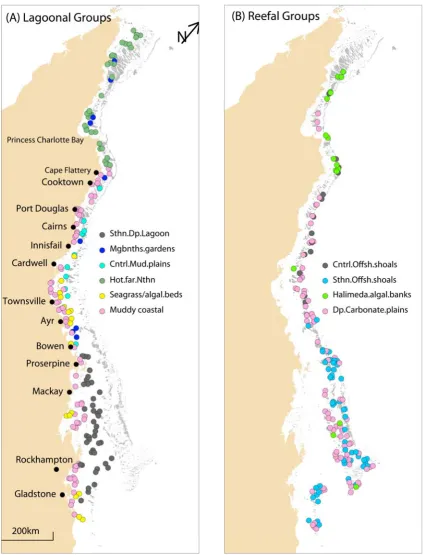
(7) substrata to produce four terminal assemblages representing deeper, offshore ‘shoals’ in the central and southern sections of the GBRMP, and deep carbonate plains (>35 metres) and shallower Halimeda/algal banks in offshore waters (Figure 6.1). The alternative splitting variables showed that the southern offshore shoals could also be distinguished by higher salinities, higher seabed current shear stress and much lower mud content of the sediments (Table 6.1). The inshore, right-hand side of the tree contained nodes and branches characterised by lower carbonate content of the sediments, the presence or absence of beds of marine plants and patches of megabenthos, and abrupt longshore faunal breaks about along ~0.37 (Bowen) in the south and ~0.74 (Cape Flattery) in the far north. The lower branching occurred about depths of ~36 metres, similar to the other side of the tree, to produce two further branches splitting on alongshore position south of Bowen and north of Cape Flattery. Each of these branches produced three terminal nodes. The shallower, inshore branch <36.75 metres terminated on one side in a hot, far northern assemblage and on the other side into a muddy, coastal node with fine sediments and a seagrass/algal bed assemblage with high coverage of marine plants. The deeper, inshore branch terminated on one side in the deep southern lagoon assemblage south of Bowen and on the other side into assemblages on the mud plains of the central section and in megabenthos ‘gardens’ (Figure 6.1). The alternative splitting variables showed that the far northern shallow assemblage could also be distinguished by lower salinities, higher temperatures and higher mud fractions in the sediments (Table 6.1). The location of BRUVS sites within the ten vertebrate assemblages were best comprehended by plotting them in inshore, ‘lagoonal’ and offshore, ‘reefal’ groups (Figure 6.2). The inshore assemblages showed distinct faunal breaks between Cooktown/Cape Flattery (along ~0.7-0.74) in the north and the top of the Whitsundays near Bowen (along ~0.37). Cape Flattery separated the ‘hot far northern’ assemblage from the ‘central mud plains’, ‘muddy coastal’, ‘seagrass/algal banks’ and ‘southern deep lagoon’, which lay between the coastal island chains and main reef matrix south of Bowen. The ‘seagrass/algal’ assemblage was best represented in a long belt in the lagoon of the central section between about Cardwell (along ~0.53) and Bowen. However, clusters of sites within this assemblage were also found on the sandy Capricorn-Bunker shelf and even inshore to the north of the Shoalwater Bay macrotidal region (Figure 6.2). The ‘central muddy plains’ were also located in a belt just inside the reef matrix between Cooktown and Bowen, slightly offshore from the ‘seagrass/algal’ assemblage. These plains had higher carbonate composition than the ‘coastal muddy plains’, which occurred almost continuously along the coast south of Cape Flattery, with the exception of a significant break along the macrotidal Broad Sound coast. Sites in that highly scoured region were members of the ‘deep 148.

(8) southern lagoon’ assemblage. Few sites, spread widely north of Bowen, were grouped in the small ‘megabenthos gardens’ assemblage. The offshore, ‘reefal’ group of assemblages also showed some strong latitudinal structure. Most of the sites in the ‘Halimeda/algal assemblage’ were located north of Cooktown, but other sites were included from the Swain group of reefs far to the south. A position offshore from Ayr (along ~0.45) separated the ‘central offshore shoals’ to the north from the widespread ‘southern shoals’ assemblage which extended to the southern extent of the study area. The ‘deep carbonate plains’ occurred offshore between reef bases and deeper than the ‘Halimeda/algal assemblage’ for most of the length of the GBR (Figure 6.2).. 149.

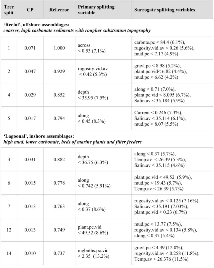
(9) Figure 6.1. A MRT based on 172 species of vertebrates and the nineteen explanatory variables. Terminal node numbers were summarised in Table 6.1, and mapped with abbreviated names in Figure 6.2. 150.

(10) Table 6.1. Values for environmental covariates producing primary and surrogate splits (nodes) on the left (1, 2, 4, 5) ‘reefal’ and right (3, 6, 7, 12, 14) ‘lagoonal’ sides (branches) of the tree in Figure 6.1. The ‘improvements’ in the model at each split are represented by the decrease in relative error from the first to the last split. The model has explained (1-0.737=26.3%) of the variation amongst the occurrence of 172 species amongst 366 BRUVS sites. The percentage improvement in each split by the primary and surrogate splitting variables shows that there were numerous correlations amongst the spatial and environmental covariates – especially the interpolated values for salinity, temperature and sediment composition.. Tree split. CP. Rel.error. Primary splitting variable. Surrogate splitting variables. ‘Reefal’, offshore assemblages: coarser, high carbonate sediments with rougher substratum topography 1. 0.071. 1.000. across < 0.53 (7.1%). carbnte.pc < 84.4 (6.1%), rugosity.vid.av < 0.26 (5.6%), mud.pc < 7.17 (4.9%). 2. 0.047. 0.929. rugosity.vid.av < 0.42 (5.3%). gravl.pc < 8.98 (5.2%), plant.pc.vid< 6.82 (4.4%), mud.pc < 6.62 (4.2%). 4. 0.029. 0.852. depth < 35.95 (7.5%). along < 0.71 (7.0%), plant.pc.vid < 8.095 (6.7%), Salin.av < 35.184 (5.9%). 5. 0.017. 0.794. along < 0.45 (8.3%). Current < 0.246 (7.3%), Salin.av < 35.114 (6.1%), mud.pc < 8.07 (5.5%). ‘Lagoonal’, inshore assemblages: high mud, lower carbonate, beds of marine plants and filter feeders 3. 0.031. 0.882. depth < 36.75 (6.3%). along < 0.37 (5.7%), Temp.av < 26.39 (5.3%), Salin.av < 35.115 (4.6%). 6. 0.015. 0.778. along < 0.742 (5.91%). plant.pc.vid < 49.52 (5.9%), mud.pc < 19.43 (5.7%), Temp.av < 26.39 (5.7%). 7. 0.013. 0.763. along < 0.37 (8.6%). rugosity.vid.av < 0.125 (7.16%), Salin.av < 35.191 (7.03%), plant.pc.vid < 0.23 (6.7%). 12. 0.013. 0.749. plant.pc.vid < 49.52 (8.6%). mud.pc < 13.77 (7.5%), rugosity.vid.av < 0.134 (5.8%), along < 0.37 (5.4%). 14. 0.010. 0.737. mgbnths.pc.vid < 2.35 (13.2%). gravl.pc < 4.39 (12.0%), rugosity.vid.av < 0.258 (11.8%), Temp.av < 26.376 (11.5%). 151.

(11) Figure 6.2. The location of BRUVS sites within the ten vertebrate assemblages divided into ‘lagoonal’ (A) and ‘reefal’ (B) groups within regions of the GBRMP (rotated). The node numbers in the legend link to Figure 6.1 and Table 6.1, where full descriptions were provided.. 152.

(12) 6.3.2 Diversity and abundance of assemblages The bar plots in Figure 6.1 showed the distribution of species abundances at each of the terminal nodes, ranked from left to right in decreasing order of prevalence in the entire data set, with each vertical bar representing the mean abundance of a species in that group. The numbers under the bar plots indicate the number n of sites within each group. Those bar plots, and summaries of species richness and abundance by assemblages in Table 6.2, showed that the most diverse assemblages were not always those comprising the most BRUVS sites. The most commonly occurring species were in relatively high abundance at all inshore assemblages, but an apparently different suite of rarer species was most abundant in the ‘reefal’ assemblages on coarser seafloor topographies of the central GBRMP and Halimeda/algal banks (Figure 6.1). The species accumulation curves showed that for the first ten BRUVS set, on average, there were about 50-80 species recorded for offshore ‘reefal’ assemblages and about 44-56 species recorded for inshore ‘lagoonal’ assemblages (Figure 6.3). With the exception of the small ‘megabenthos gardens’ assemblage (just nine sites) and the relatively depauperate ‘hot far northern’ assemblage, the curve shapes for the inshore assemblages showed a coarsely similar trend toward an asymptote above one hundred species. In contrast, trends for all the offshore, ‘reefal’ assemblages indicated latent diversity well above 120 species. The steep slopes of the curves for assemblages on rougher ‘shoal’ seafloors and ‘Halimeda/algal banks’ were particularly steep, with the most diverse fauna (~25 species per BRUVS set) recorded on the small, ‘central offshore shoals’ assemblage (14 sites with 96 species) (Figure 6.3, Table 6.2).. 153.

(13) Table 6.2. Summaries of richness and abundance in the ten terminal fish assemblages. See Table 6.1 and Figure 6.1 for an explanation and summary of MRT node numbers and abbreviated node names. Overall richness and (raw) abundance are shown for the membership of each node, together with ranges, means and standard deviations in these parameters for n sites within nodes. The MRT was based on 172 species of vertebrates, with prevalence >3, and 19 spatial and environmental covariates.. node. n sites. Node name. ∑richness (S). S range. S mean. ∑abund (N). N range. N mean. ‘Reefal’, offshore assemblages: coarser, high carbonate sediments with rougher substratum topography Smoother seafloors – Rugosity.vid.av <=0.146 8. 80. Dp.Carbonate.plains. 117. (3-28). (10.6 ± 4.9). 5244. (10-248). (65.5 ± 43.7). 9. 17. Halimeda.algal.banks. 86. (6-28). (19.1 ± 6.4). 2457. (25-525). (144.5 ± 124). Roughest seafloor topography – Rugosity.vid.av >0.146 10. 51. Sthn.Offsh.shoals. 111. (6-39). (15.6 ± 6.6). 6256. (26-585). (122.7 ± 90.4). 11. 14. Cntrl.Offsh.shoals. 96. (13-43). (24.9 ± 9.5). 1107. (25-212). (79.1 ± 56.8). ‘Lagoonal’, inshore assemblages: high mud, lower carbonate, beds of marine plants and filter feeders Depth <= 36.75 m Central and Southern GBRMP; Along<0.74 24. 71. Muddy coastal. 106. (2-21). (10.8 ± 4). 4109. (6-336). (57.9 ± 52.5). 25. 17. Seagrass/algal.beds. 66. (11-28). (16.4 ± 4.2). 3269. (49-1096). (192.3 ± 240.2). Along >= 0.74. 154.

(14) node. n sites. Node name. ∑richness (S). S range. S mean. ∑abund (N). N range. N mean. 13. 35. Hot.far.Nthn. 76. (8-23). (14.7 ± 3.4). 5363. (59-549). (153.2 ± 108.6). Deeper waters >36.75 m Central section of GBRMP 28. 11. Cntrl.Mud.plains. 50. (8-21). (14.3 ± 3.3). 755. (18-122). (68.6 ± 27.3). 29. 9. Mgbnths.gardens. 55. (11-19). (14.3 ± 2.4). 1890. (71-575). (210 ± 185). 92. (8-26). (15.4 ± 4.6). 4705. (39-230). (114.8 ± 55). Southern section; Along < 0.37 15. 41. Sthn.Dp.Lagoon. 155.

(15) Figure 6.3. Species-accumulation curves for the ‘reefal’ (a) and ‘lagoonal’ (b) assemblages of vertebrates. For definitions of the assemblages names see Table 6.1.. 156.

(16) 6.3.3 Indicator species for assemblages The analysis of DLI indicator values was conducted for all nineteen nodes of the regression tree, from the root node (representing the entire GBRMP) to the ten terminal assemblages (Figure 6.4, Table 6.3). The assemblages with few lower DLI values were dominated within the spatial hierarchy by the other assemblages with many species indicators – in the sense that all species in these terminal nodes also occurred in higher numbers elsewhere. Thus, the indicator species with DLI maxima at the root node were generally ubiquitous and widely distributed. Of the 172 species, only 48 (28%) had moderately high DLI values (between twenty and fifty), and only six species had high DLI ≥50. Inspection of Figure 6.4 shows that assemblage size was not a good indicator of specificity and fidelity of member species, with the smallest assemblage (nine sites in ‘megabenthos gardens’) represented in DLI analysis by only a single species. The large ‘muddy coastal’ and ‘deep carbonate plains’ assemblages comprised over forty percent of all BRUVS sites (Figure 6.3), but their member species were ubiquitous in other branches and nodes of the tree and they contained no indicator species with moderate to high values. In contrast, the terminal assemblages on the offshore, ‘reefal’ side of the tree had almost seven times as many species with DLI ≥ 20 (n=20), compared to the inshore, ‘lagoonal’ assemblages. The ‘Halimeda/algal banks’ and ‘central offshore shoals’ comprised only 14-17 BRUVS sites, yet they had a diverse, abundant vertebrate fauna (Figure 6.3, Table 6.2) including relatively many species recorded there in highest numbers (Table 6.3). The lethrinids, mullids, scarids, labrids, lutjanids and balistids of the ‘central offshore shoals’ were remarkably similar to the faunal list from coral reef bases sampled in Chapter 3.2.2 (see Figure 3.5). The two ‘shoal assemblages’ were branches of a more widespread fauna inhabiting topographically complex seafloors (rugosity.vid.av ≥ 0.416) with coarse sediments high in biogenic carbonate (node 5). This fauna included labrids and lethrinids known to consume benthic invertebrates, two planktivorous pomacentrids, and a chaetodontid suspected to eat a wide variety of invertebrates and encrusting organisms. There was also evidence of a fundamental faunal break around the vicinity of the top of the Whitsundays-Bowen (along ~0.37), affecting the composition of both inshore and offshore assemblages. In the middle branches of the tree there were a wide variety of fish, elasmobranchs and sea snakes that had highest DLI to the north of Bowen (see node 14 in Figure 6.1 and Table 6.3). These included hammerhead sharks and a shovelnose ray as well as pelagic planktivores and piscivores. The abundant, gregarious Paramonacanthus filicauda and the small, deepbodied Carangoides malabaricus_grp were found almost exclusively south of this position in. 157.

(17) the ‘southern deep lagoon’ assemblage over smooth, muddy seafloors. Further offshore, the presence of Upeneus filifer and Parapercis xanthozona_grp was also limited exclusively to this southern region, but their DLI values in the ‘southern offshore shoals’ assemblage were only moderate because they were not abundant, or present at all sites in the assemblage. The vicinity of Cape Flattery (along ~0.74) represented another faunal break, but this was weaker in terms of the DLI values of representative species there. It was notable that the Australian blacktip shark (Carcharhinus tilstoni_grp), two planktivorous, pelagic carangids (Alepes and Atule) and a small (perhaps juvenile) tetraodontid pufferfish had highest DLI in the warmer, less saline waters of the ‘hot far northern’ assemblage. There was no clear progression of families across the shelf as predicted for tropical shelf provinces by Longhurst & Pauly (1987). Instead, there was clear evidence of species replacements within genera amongst assemblages. This was particularly evident for the nemipterids (Pentapodus, Scolopsis and Nemipterus), small carangids (Carangoides), monacanthids. and. lethrinids.. For. example,. amongst. the. monacanthid. filefishes. Paramonacanthus japonicus was most abundant in offshore ‘Halimeda/algal banks’, and the inshore assemblages were inhabited by P. otisensis (depth<37m), Monacanthus chinensis (‘seagrass/algal beds’), P. lowei (‘central mud plains’) and P. filicauda (‘southern deep lagoon’). Similarly, the abundance of small lethrinids split between Lethrinus genivittatus (‘seagrass/algal beds’), L. semicinctus (‘Halimeda/algal banks’) and L. ravus (‘central offshore shoals’). Interspecific differences in these, and other, genera are explored further in the next chapter.. 158.

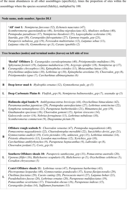
(18) Figure 6.4. Node names and top ten species indicators (DLIs) for the terminal nodes (leaves) of the MRT defined by the 19 explanatory variables. Terminal node numbers were summarised in Table 6.1 and mapped with abbreviated names in Figures 6.1 and 6.2. 159.

(19) Table 6.3. Summaries of the Dufrêne- Legendre Index (DLI) for all 172 species in all nine higher nodes (branches – B) and ten terminal nodes (leaves – L). For a given species and a given group of sites, the DLI was defined as the product of the mean species abundance occurring in the group divided by the sum of the mean abundances in all other assemblages (specificity), times the proportion of sites within the assemblage where the species occurred (fidelity), multiplied by 100.. Node name, node number, Species DLI ‘All’ root 1: Nemipterus furcosus (52), Echeneis naucrates (47), Scomberomorus queenslandicus (46), Seriolina nigrofasciata (42), Abalistes stellatus (40), Pentapodus paradiseus (37), Nemipterus theodorei (35), Lagocephalus sceleratus (34), Saurida_grp (30), Carangoides fulvoguttatus (27), Upeneus tragula_grp (23), Parapercis nebulosa_grp (19), Feroxodon multistriatus (12), Lutjanus sebae (11), Lutjanus vitta (8), Gymnothorax sp (3), Caranx ignobilis (2) Tree branches (nodes) and terminal nodes (leaves) on left side of tree. B. ‘Reefal’ Offshore 2: Carangoides coeruleopinnatus (40), Pristipomoides multidens (19), Sphyraena forsteri (19), Lutjanus malabaricus (19), Argyrops spinifer (18), Nemipterus sp (17), Carangoides chrysophrys (16), Epinephelus coioides (11), Meiacanthus luteus (10), Oxycheilinus unifasciatus (10), Lethrinus sp (10), Epinephelus areolatus (9), Choerodon_grp (8), Pristipomoides typus (7), Carcharhinus albimarginatus (6). B. Deep lower mud 4: Hydrophis ornatus (12), Gymnothorax pale_sp (5). L. Deep Carbonate Plains 8: Flatfish_grp (9), Nemipterus balinensoides_grp (7), seasnake sp (5). L. Halimeda algal banks 9: Amblypomacentrus breviceps (44), Oxycheilinus bimaculatus (42), Paramonacanthus japonicus (29), Pentapodus aureofasciatus (27), Lethrinus semicinctus (22), Symphorus nematophorus (21), Parupeneus barberinoides (21), Himantura fai_grp (19), Gnathanodon speciosus (16), Choerodon gomoni (15), Aprion virescens (14), Galeocerdo cuvier (14), Nebrius ferrugineus (11), Lethrinus nebulosus (10), Scomberomorus commerson (9), Diagramma pictum (9). B. Offshore rough seabeds 5: Choerodon venustus (47), Pentapodus nagasakiensis (40), Pomacentrus nagasakiensis (22), Chaetodontoplus meredithi (22), Suezichthys devisi_grp (21), Gymnocranius audleyi (19), Coris pictoides (16), unknown_grp (15), Lethrinus miniatus (14), Pristotis obtusirostris (13), Loxodon macrorhinus (12), Xyrichtys_grp (10), Carcharhinus amblyrhynchos (9), Parupeneus heptacanthus (9), Labroides sp (8), Choerodon jordani (7), Coris_grp (6). L. Southern Offshore shoals 10: Parapercis xanthozona_grp (33), Pomacentrus australis (20), Upeneus filifer (16), Halichoeres scapularis (8), Halichoeres sp (5), Oxycheilinus celebicus (5), Coradion chrysozonus (5). L. Centrl Offshore shoals 11: Lethrinus ravus (47), Parupeneus barberinus (43), Plectropomus leopardus (40), Gymnocranius grandoculis (37), Scarus flavipectoralis (29), Cheilinus fasciatus (29), Caesio cuning (28), Pterocaesio marri (27), Lutjanus bohar (21), Pseudobalistes fuscus (20), Lethrinus ornatus (20), Parupeneus multifasciatus (19), Pomacanthus sexstriatus (17), Triaenodon obesus (16), Parupeneus indicus (15), Carangoides ferdau (14), Sufflamen fraenatum (13). 160.

(20) Node name, node number, Species DLI Tree branches (nodes) and terminal nodes (leaves) on right side of tree. B. ‘Lagoonal’ Inshore 3: Selaroides leptolepis (48), Nemipterus hexodon (39), Lagocephalus lunaris (17), Epinephelus sexfasciatus (14), Terapon theraps (13), Carangoides talamparoides_grp (11), Scomberoides commersonnianus (6), Arius thalassinus_grp (2). B. Shallow inshore 6: Paramonacanthus otisensis (34), Carangoides hedlandensis (21), Lutjanus carponotatus (1). B. Inshore southern and central 12: Carangoides dinema_grp (21), Nemipterus peronii (20), Leiognathus longispinis (5). L. Muddy coastal 24: Platycephalidae_grp (8), Pomadasys maculatus (4). L. Seagrass/algal beds 25: Lethrinus genivittatus (26), Choerodon cephalotes (11), Selar boops (10), Torquigener_grp (9), Siganus fuscescens_grp (8), Monacanthus chinensis (8), Stegostoma fasciatum (5), Chiloscyllium punctatum (5). L. Hot far Northern 13: Carcharhinus tilstoni_grp (19), Atule mate (17), Alepes apercna (16), Lagocephalus_grp (12), Rhizoprionodon taylori_grp (9), Terapon puta (5). B. Deep inshore 7: Caranx bucculentus (14), Terapon jarbua (12), Gymnothorax dark_sp (7), Siganus argenteus (3). B. Deep central section 14: Cybiosarda elegans (91), Sphyrna lewini (84), Sphyrna mokarran (66), Lapemis hardwickii (62), Decapterus russelli (48), Rachycentron canadum (45), Rhynchobatus djiddensis (43), Aipysurus laevis (39), Gymnothorax minor (33), Carangoides gymnostethus (23), Scolopsis taeniopterus (17). L. Central Mud plains 28: Nemipterus nematopus (25), Paramonacanthus lowei (23), Ostracion_ grp (4), Carangoides orthogrammus (4). L. Megabenthos gardens 29: Leptojulis cyanopleura (12), Carcharhinus dussumieri (10), Sphyraena jello (8), Lethrinus lentjan (5), Lethrinus laticaudis (5). L. Southern Deep Lagoon 15: Paramonacanthus filicauda (52), Carangoides malabaricus_grp (27), Choerodon monostigma (6), Parastromateus niger (6), Lutjanus adetii (3). 161.

(21) 6.4. DISCUSSION. The application of the BRUVS technique enabled the measurement of relative abundance of many functional groups of vertebrates along the major gradients on the GBR shelf. Demersal, semi-pelagic and pelagic fish, sharks, rays and seasnakes from several centimetres (e.g. Paramonacanthus) to several metres in length (e.g. Galeocerdo, Sphyrna) were recorded in standard surveys with enough data to allow the definition of ten assemblages constrained by major hydrological, sedimentary and spatial factors. 6.4.1 Cross-shelf patterns I propose that cross-shelf variation in sedimentary processes and along-shelf variability in oceanic influences described in Chapter 5.4 shaped the boundaries identified here amongst assemblages. The wide range of inter-reef habitats is dominated in different regions of the GBRMP by combinations of cyclonic events, tides, currents and upwellings, waves, riverine inputs and seasonal winds (Larcombe & Carter 2004; Porter-Smith et al. 2004). These forces govern the topography, grain size and composition of sediments, the chemical properties of overlying waters and therefore the nature of infaunal, phototrophic or filter-feeding epibenthic communities (Fabricius et al. 2005; Fabricius & De’ath 2008). In turn, these habitats influence the recruitment, feeding success and mortality of fish assemblages inhabiting them. The cross-shelf boundaries separating the vertebrate assemblages are related to the three sedimentary belts in seabed composition and topography parallel to shore that have been generally recognised in the GBRMP. In the central section of the GBR, the terrigenous inner shelf prism of bioturbated sand and mud extends 15-20km offshore to water depths of 20-22m. The lagoon below those depths (22-40m) is starved of terrigenous sediment and has a thin veneer of mixed shelly, muddy sand and shell hash overlying weathered Pleistocene clay, which is exposed by cyclones to form outcrops on the seabed. The seafloor amongst the mid-shelf and outer-shelf reefs (40-80m) is also starved of terrigenous sediment, but there are Pleistocene reef edges and outcrops, accumulations of old reef framework and detrital carbonate sediments where modern coral reefs emerge. Local influences, such as tidal jets, cause accumulation of carbonate mud or Halimeda algal banks (bioherms) in the reef matrix, whilst elsewhere the flat outer shelf plain is covered thinly by shelly calcsand. These zones are maintained through the influence of south-easterly trade winds driving along-shelf drift northward, and by the regular passage of tropical cyclones causing strong northward currents in the lagoon (Larcombe & Carter 2004).. 162.

(22) The MRT analyses of 172 species reflected this long-term stratification by separation of four ‘reefal’ assemblages, from six inshore ‘lagoonal’ assemblages, where sediments had less than ~84% carbonate content and an index of seafloor topography, or grain size, was at the coarser end of the spectrum beyond mud. The ‘shoals’ assemblages comprised less than nine percent of all sites but were characterised by a high diversity of species normally associated with emergent reefs and reef bases such as the parrotfish Scarus flavipectoralis, the coral trout Plectropomus leopardus and the fusilier Caesio cuning. The location of sites in the offshore ‘Halimeda/algal banks’ assemblage reflected the prevailing knowledge that meadows of the alga Halimeda occur in clear waters throughout the entire outer shelf of the GBRMP, but by far their richest development, into extensive, 15-20m thick bioherms is driven by tidal jetting of nutrients behind the chain of Ribbon reefs north of Port Douglas (16°S) (Pitcher et al. 2008). A significant number of members of the ‘Halimeda/algal banks’ assemblage were not common elsewhere. These included species from families normally associated with coral reefs, such as labrids, mullids, pomacentrids, a lutjanid and a lethrinid. Many of these were recorded as juveniles in the tape interrogation, and it is highly likely the interstitial spaces amongst the algal fronds and skeletons offered both shelter sites and abundant food in the form of invertebrate epifauna and infauna. 6.4.2 Along-shelf patterns The latitudinal boundaries between the assemblages can be related to the configuration of the shelf and reef matrix, currents and tides, which cause notable exceptions to the model of Larcombe & Carter 2004. Much of the area south of Bowen is macrotidal, with a maximum tidal range of 8.2 metres in Broad Sound near Mackay. Porter-Smith et al. (2004) predicted that mobility and grain size properties of the sediment in this region were dominated by tidal currents, in contrast with the rest of the GBRMP. Therefore an inner ‘terrigenous fine mud belt’ does not occur along much of the coast (particularly in the region of Broad Sound and Shoalwater Bay) because of sediment mobilisation and deposition offshore. In this region, the water was often too turbid for effective BRUVS sampling, but there were indications of a break in the ‘muddy coastal’ assemblage where the ‘southern deep lagoon’ assemblage penetrated towards the coast. Filter-feeding sponges, gorgonians, alcyonarians and sea whips are known to establish ‘gardens’ in such waters where high seabed currents expose holdfasts for attachment and bring streams of pelagic food (Pitcher et al. 1999; 2000; Haywood et al. 2008). Studies elsewhere suggested that these ‘megabenthos gardens’ would be a major habitat for inter-reefal fishes of the GBR.. 163.

(23) Studies of the indirect effects of fishing on Australia’s Northwest Shelf inferred that the reduction in megabenthos by trawling, with heavy gear for fish, may have caused a species shift from high value lutjanids and lethrinids to low value nemipterids and saurids. Still-camera frames showed more Lethrinus and Lutjanus in remaining areas of large (>25cm) benthos, wheareas Nemipterus and Saurida showed a significantly higher probability of occurrence in areas without large epibenthos (Sainsbury et al. 1992). Instead, patches of megabenthos were rare amongst the sites sampled with BRUVS in the GBR and the ‘megabenthos gardens’ assemblage was the smallest recognised in the MRT analysis. Species accumulation curves suggested that there was a diverse fauna associated with this (undersampled) assemblage, but few species showed maxima in fidelity and specificity there. There was no indication that economically important lutjanids or serranids were associated preferentially with such epibenthos in the GBR, although two uncommon species of Lethrinus did have maximum DLI in the ‘megabenthos gardens’. Deepwater seagrasses (only Halophila spp.) are an extensive but poorly known fish habitat in depths of 15-61 metres in the middle of the lagoon and outer part of the shelf where waters are clear enough for light penetration (Carruthers et al. 2002; Coles et al. 2009). Seagrass was predicted to be present on at least 40,000km2 of the inter-reef lagoon in a recent study by Coles et al. (2009), with distributions explained mainly depth, sediment type and turbidity. They form extensive meadows in a band from Princess Charlotte Bay to just south of Townsville, within a 15-25 metre depth band associated with the presence of terrigenous sediments and mid-range particle sizes. This region bathes the coastal wet-dry tropics with a moderate tidal range, high annual rainfall and numerous mangrove estuaries. There is potentially a large supply of seagrass seeds and vegetative fragments, and enough riverine and oceanic nutrient inputs to sustain seagrass growth. No major deepwater seagrass meadows exist in the Mackay region of high current stress, high turbidity and coarse mobile sediments, but they are dense in some southernmost parts of GBR south of 23°S (Coles et al. 2009). A distinct, diverse assemblage of vertebrates was found in ‘seagrass/algal beds’ wherever they occurred amongst the BRUVS sites, but mainly in a mid-shelf belt in the central GBR and on the Capricorn-Bunkers sand shelf. Unlike the ‘Halimeda/algal banks’ assemblage there were relatively few species indicators in these vegetated sites, with the notable exception of the common and abundant Lethrinus genivittatus and the herbivorous Siganus fuscescens_grp. The filefish Monacanthus chinensis is thought to include epiphytes in its diet, and this species too had maximum DLI in this assemblage. This implied that ‘seagrass/algal banks’ were inhabited by a large number of species, but these were also found elsewhere in high abundance. 164.

(24) The westward impingement and bifurcation of the South Equatorial Current (SEC) against the continental shelf peaks in the central region between 14°S and 20°S provided a further division of the GBRMP that explained the cross-shelf and latitudinal boundaries I described amongst assemblages. The reef matrix is significantly more ‘permeable’ in this section between the Ribbon reefs in the north and the Pompey reefs off Proserpine to the south. The density of barrier reefs is much lower and the westward flowing SEC readily traverses the numerous passages shoreward in this central region. The bifurcation produces the East Australian Current (EAC), with a southerly and stronger set over the summer months. There is direct infiltration of the SEC across the central shelf and regional upwelling induced by the southerly-setting EAC (Wolanski 1994). The net outcome is an influx of oceanic water which penetrates the reef matrix as far as the mid-shelf. The location of contiguous sites in the ‘seagrass/algal beds’ assemblage in this region suggests the clear, enriched waters are supporting marine plant growth there. The northward flow in the lagoon induced by the trade winds effectively halts this influx, forming a coastal boundary layer (Brinkman et al. 2002). The result is a cross-shelf gradient that isolates nearshore waters from the outer lagoon in the central section, and the formation of three different regions of water movement along the GBRMP. The amplitude of seasonal variation in sea surface temperature (SST) and salinity were also important in splitting the branches and nodes of the MRT. These gradients are undoubtedly influenced by the configuration of the reefs; Hancock et al. (2006) found that inner lagoon diffusivity was about 2.5 times higher in the central section compared to the north. Water within twenty kilometres of the central coast is flushed with outer lagoon water on a time scale of 1845 days, with the flushing time increasing northwards. Major rivers of Cape York, such as the Normanby, flow out into this constricted northern region. This contributes to the dilution of the water column, which is warmer and less dense than the southern extremes of the GBR. Salinities in the southern lagoon are significantly higher than those in the central and northern sections, and seasonal variation is lower. Summer SST are ~2-3°C lower in the region south of Bowen compared to the far north, and in winter a relatively cold coastal water body forms there (Condie & Dunn 2006). There was evidence of northward penetration of a subtropical vertebrate fauna to meet the north tropical fauna of hotter climates in the vicinity of the top of the Whitsunday Islands/Bowen region (along ~0.37). This boundary was most remarkable for the schooling Paramonacanthus filicauda, which is known to occur as far south as Sydney. Sub-tropical sparids (Pagrus auratus, Acanthopagrus australis), carangids (Pseudocaranx dentex, Seriola lalandi, S. dumerili), the scombrid Sarda orientalis and the glaucosomatid Glaucosoma scapularis were seen in this southern region, but were not prevalent enough to be included in the MRT analyses. It is highly 165.

(25) likely that the area of the inter-reef lagoon south of Bowen is a biotone, or area of transition (IMCRA 1998), and there was strong evidence of this in analysis of species ranges in Chapter 5.2.3.3. 6.4.3 Comparison with other tropical shelves The assemblages described here bear little resemblance to the generalisations predicted by Longhurst & Pauly (1987), Lowe-McConnell (1987) and Longhurst (2007) for other tropical shelves where there are no barrier reefs, and where slopes are steeper under a permanent or seasonal thermocline. These patterns have been inferred under the selectivities imposed by fish trawls, which were discussed in Chapter 4.4, so sharks, rays and other large carnivores (such as carangids and scombrids) are seldom mentioned. The nature of the fish communities on those shelves has been described as being dominated both by deposit type and by water mass. In softer sediments of turbid shallows there are ariid catfishes, sciaenid croakers and polynemid threadfins in India, West Africa, the Caribbean and Brazil. Further offshore, sandy deposits and stony bottoms are inhabited by assemblages characterised by lutjanid snappers, haemulid grunts and sparid sea breams. Over fifty percent of the standing stock has been reported to be comprised of these families, with the addition of serranids, in the Arabian Gulf (Longhurst 2007), but these figures were measured from retained commercial catches and the real nature of assemblages is unknown. Instead of cross-shelf replacement of these (or other) fish families in the GBRMP, I recorded the same families were represented in different assemblages by different genera or by different species within genera. This may indicate interspecific interactions, pressures of predation and competition, the vicariance of previous large-scale disturbances, or the long-shore intermixing of species from different biomes. Many prevalent species (such as Nemipterus furcosus, Echeneis naucrates, Pentapodus paradiseus and Seriolina nigrofasciata), located by indices of fidelity and specificity (DLI) in the lower branches and root node of the MRT, occurred in several assemblages. It was the differences in abundances of these prevalent ‘shared’ species that contributed most to dissimilarity between the large ‘deep carbonate plains’ and ‘muddy coastal’ assemblages in which no species had moderate to high DLI values. A differentiation of communities based on abundant fishes is considered more robust than one based on uncommon species that may represent artefacts of sampling (Williams & Bax 2001; Greenstreet & Piet 2008). Past insights into the factors structuring tropical assemblages have been gained from extreme shifts in communities through ‘fishing down the food chain’ (Pauly et al. 1998; Pauly & Chuenpagdee 2003; Laurans et al. 2004; Carbines & Cole 2009) or through natural ‘regime. 166.

(26) shifts’ caused by inter-decadal climatic cycles (Botsford et al. 1997). Unlike the GBRMP (Brodie & Fabricius 2009), the Gulf of Thailand has relatively high primary productivity, boosted by rapid increase in nutrients from farm runoff and prawn farm effluent. These inputs have been associated with noxious algal blooms in the inner Gulf off Bangkok. At the same time, trawl catch rates declined ten-fold from ~ 300kg hr-1 in 1961 and 50kg hr-1 in the 1980s to 20-30kg hr-1 in the 1990s. The catch composition changed within species (from large to small individuals) and between species (toward a mix of predominantly small, short-lived species). Rapid value-adding of small ‘trash fish’ as mariculture feed subsidised the continued overfishing of larger species. By the mid 1990s the ratios of fishing mortality: natural mortality were ~0.8 to ~0.96 for the major species of lutjanids, serranids, carangids and nemipterids, yet biomasses had fallen to below ten percent of their original levels (Stobutzki et al. 2006). Whilst the fishing industry perceived ‘pollution’ as the proximate cause, it is now seen as highly plausible that the fisheries themselves have contributed to the increase of jellyfish and other consumers of herbivororus zooplankton by removing the upper parts of natural food webs. In other words, unabated over-fishing has led to a trophic cascade causing phytoplankton blooms and the ensuing depletion of oxygen in the enclosed inner Gulf. Elsewhere the remarkable rise in biomass of some highly evolved balistid triggerfish and tetraodontid blowfish cannot be determined because of lack of knowledge of the environmental drivers shaping the assemblages in which they occur. Population outbursts have been attributed to changes in ocean circulation and upwelling through ‘unknown mechanisms’, or to resilience to capture and discarding. In 1972-82, the triggerfish Balistes capriscus came to dominate the biomass and ecosystem of the Ghanaian fishery for nearly twenty years. The catch rose from only one tonne in 1972 to 13,000 tonnes in 1979 (Joanny & Menard 2002). These triggerfish are considered highly edible in West Africa, but the proliferation in the Gulf of Guinea LME of the tetraodontid globefish Lagocephalus laevigatus (Koranteng 2001) would not be so profitable because it is extremely toxic. In Colombia a similar rise in abundance of B. capriscus and tetraodontids has been observed in the last thirty years of the 20th century, but both are discarded and their resistance to the effects of capture has been cited as reasons for their population growth (García et al. 2007). Studies of the indirect effects of fishing have also indicated the major importance of epibenthic habitats and species interactions in shaping fish assemblages. On Australia’s northwest shelf, Sainsbury et al. (1992; 1997) found that Nemipterus and Saurida showed a significantly higher probability of occurrence in areas without large epibenthos. In the altered habitat, and under a release from predation or competition, the shortlived (~1 year) Saurida species increased by two orders of magnitude and their longer-lived (6-7 years) congeners increased by one order of 167.

(27) magnitude (Thresher et al. 1986). The rise of such voracious piscivores was considered to have had a profound effect on the survival of the remaining members of the assemblages on the northwest shelf. An increase in populations of Saurida was also observed after twenty years of prawn trawling in the Gulf of Carpentaria, accompanied by a 500-fold decrease in the catch rates of Paramonacanthus spp. (Harris & Poiner 1991). However, those authors considered the decline to be due to changes in the mud content of the sediments on parts of the trawl grounds and made no mention of the possible role of a rise in their predators. All these examples underscore the need for a better understanding of the factors shaping fish populations and assemblages on tropical shelves.. 168.

(28) 7.. SPATIAL MODELS EXPLAINING AND PREDICTING THE OCCURRENCE OF COMMON INTER-REEF VERTEBRATES OF THE GREAT BARRIER REEF MARINE PARK. 7.1. INTRODUCTION. The ‘extreme deconstruction principle’ (Terribile et al. 2009) proposes that patterns in species richness and species assemblages may be viewed as macroecological consequences of population-level processes acting on species’ geographical ranges. Chapters 5.4 and 6.2 of this thesis have shown that spatial patterns in vertebrate species richness and assemblage structure can be explained by mud and carbonate content of the sediments, the topographic complexity of the seabed, salinity, temperature, seabed current shear stress and the location and nature of epibenthic plants and filter-feeding communities in the GBRMP. The next logical step in this exploration of vertebrate biodiversity is to determine which species in the data set are the most predictable, and to produce a collection of univariate models to relate species occurrence to the suite of environmental covariates. This will enable an assessment of which species share common responses (either positive, negative or neutral) to the environmental predictors, and which species are generalists or specialists with respect to features of the habitat at regional scales. Ecological theory predicts that habitat specialists (such as corallivores) are more vulnerable to disturbances, especially those events or processes that alter the epibenthic microhabitats they rely on for food, shelter or recruitment sites (Jones et al. 2004; Munday et al. 2008; Pratchett et al. 2008). Species models incorporating both environmental and spatial information are not common for tropical shelves, because most of the spatial information at regional scales is derived using catch-per-unit-of-effort (CPUE) data from commercial fisheries logbook programs. Biomass estimates were of prime concern in these models, and management interventions are often based on spatial or temporal closures to fishing, so there has not been a major need for understanding of the extrinsic environmental mechanisms causing spatial patterns. The advent of ‘ecosystem based’ fisheries management, and the realisation that provincial-scale ‘regime shifts’ can occur in fished assemblages when environments change (Ehrich et al. 2009; Halliday & Pinhorn 2009; Jose Juan-Jorda et al. 2009) have stimulated a much greater recognition of the need for an understanding of the intrinsic and extrinsic processes underlying spatial patterns (for example, Ehrich et al. 2009 and Jose Juan-Jorda et al. 2009). Major amendments in 1996 to the Magnuson-Stevens Fishery Conservation and Management Act 169.

(29) (USA) require fisheries managers to define ‘essential fish habitat’ and address the impact of fishing gear in their management plans. It is therefore necessary first to understand the association between fish and their habitat before considering what might qualify as essential fish habitat. A major theme of studies on both temperate and tropical shelves has been to identify the subtle relationships between fishes and sediment type (Koranteng 2001; Kouame et al. 2008; Sanchez et al. 2008; Ordines & Massuti 2009; Svane et al. 2009; Torres 2009) or depth (Garces et al. 2006b; Katsanevakis & Maravelias 2009). However, this approach does not quantify habitat complexity (Kaiser et al. 1998), which may be provided by both abiotic features of the substratum and overlying water column and by biogenic structures formed by infauna and epifauna. Such biotic complexity can be formed by the live (or dead) shells, holdfasts and thalli of plants and animals, and the burrows and excavations of bioturbating infauna (Gribben et al. 2009; Noji et al. 2009; Webb et al. 2009). Other than coral reefs, notable examples from the tropics include ‘shell beds’, ‘megabenthos gardens’, Halimeda bioherms, deepwater seagrass beds and Callianassa banks (Siebert & Branch 2006; Chavanich et al. 2009; Pitcher et al. 2009). ‘Ecosystem engineers’ are now known to excavate shallow depressions in tropical seafloors in their search for food in the case of large rays, or establishment of ambush and shelter sites in the case of Epinephelus coioides (pers. comm., Thomas Stieglitz, JCU; Marcus Stowar, AIMS). There is some speculation that the removal of surficial sediments may facilitate the colonisation of some epibenthos by exposing hard sites for post-larval recruitment. Models of the distributions of tropical vertebrates are lacking on the sub-regional and regional scales relevant to conservation, fisheries management and detection of environmental change. Identifying robust models may be the first step towards predicting responses of these species to changes in the environmental conditions, similar to modeling applications in the terrestrial realm (Beger & Possingham 2008). Such knowledge has identified shifts to deeper water or cooler latitudes for species in the North Sea (Dulvy et al. 2008) and Northeast United States continental shelf ecosystem (Nye et al. 2009) and attributed them to global warming. Elsewhere, an awareness of hypoxic ‘dead zones’ (e.g. in the Gulf of Mexico) has produced an imperative to predict fish distributions as a function of seasonal or episodic changes in oxygen concentration and other physiological constraints on fish growth and survival (Hazen et al. 2009). Spatial models of biomass in fisheries also benefit when refined with the dual effect of the sediment composition and three-dimensional complexity of habitats (Gribble et al. 2007). This has been thoroughly demonstrated in deep water for the Sebastes rockfishes at all relevant spatial scales from centimetres to entire shelves (Yoklavich et al. 2000; Yoklavitch et al. 2002; Anderson & Yoklavich 2007; Yoklavich et al. 2007; Love & Yoklavitch 2008; Rooper 2008; 170.

(30) Anderson et al. 2009; Love et al. 2009). When matched with precise maps of fishing activity, it is possible to use such species models to assess ‘risk’ of a metapopulation to the removals, and habitat disturbance, by fishing activities. In this chapter I investigate the influence of key environmental covariates on the occurrence of the ‘most predictable’ species at scales useful to management of human activities in the GBRMP. I have four main aims that extend my investigation of key drivers of patterns in species richness and species assemblages down to the level of the individual species comprising these patterns. Firstly, I determine which of the more prevalent species in the large BRUVS dataset were the most predictable in terms of the full suite of explanatory variables and I examine the errors in prediction. Secondly, I compare the performance of models under three scenarios incorporating all the predictors, only position and depth, and only the environmental covariates. Thirdly, I use partial regression plots to illustrate the shape of individual species responses to individual environmental covariates that vary along the cross-shelf and long-shore gradients described in previous chapters. These plots provide a visual means of interpreting the similarities in responses of species within assemblages, and the differences in responses that might be responsible for species replacements along gradients. Finally, I wish to show how the spatial distributions of populations at the shelf scale can be coincident with the location of fine and coarse sedimentary facies, gradients in properties of the water column, and the epibenthos. To do this I present maps of predicted species distributions in comparison to measurements of mud, carbonate, gravel, temperature, salinity and marine plants. These maps provide the easiest visualisation possible for complex species-environment relationships in the final discussion of the results presented in this thesis. 7.2. METHODS. The survey design, 366 BRUVS sites and environmental covariates have been described in detail in Chapter 5.2. The BRUVS data was analysed with all 28 spatial and environmental explanatory variables in three main ways. Firstly, the 36 species that occurred on at least nine percent (nsites= 34) of the 366 BRUVS sites were selected. These were the most prevalent in terms of the number of sites on which they occurred, not necessarily the most abundant nor the most widespread in spatial terms. Using boosted trees, the occurrence (presence or absence) of each of these species at a site was predicted from the environmental data. Boosted trees are widely regarded as one of the best predictive methodologies, and handle complex data sets and a broad range of loss functions (see Chapter 2.4.2 for explanation). For the occurrence data analysed here, the Bernoulli loss function was used. This is a logistic regression for classification problems where the outcomes are between zero and one (Ridgeway 2000). For. 171.

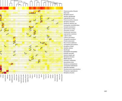
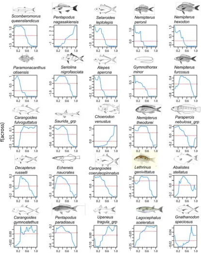
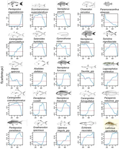
(31) tree-based methods the approximate ‘relative influence’ of a variable is the empirical improvement by splitting on that variable at a particular point (node). Secondly, logit (log2(p/1-p)) functions of the probability of occurrence (p) of each species predicted by the levels of each predictor were plotted together in ‘heatmap’ analysis for all species and predictors, and separately for the top eleven predictors and 25 most predictable species. The heatmap presented coloured cells (the logit plots for each predictor adjusted to a unit value for each species) bordered by dendrograms from cluster analyses of the ‘relative influence’ (hereafter termed ‘influence’). The clustering used the complete linkage method to find similar clusters in a Euclidean distance matrix. The upper dendrogram in a heatmap clusters the distances in influence between the rows of a matrix where the rows were the 28 environmental covariates and the columns were the 36 species. The other dendrogram on the left of the heatmap does the same clustering on a transposition of the matrix, so rows represent species and columns are the predictors. Thus the upper dendrogram clusters the predictors by the similarity in the magnitude of their influence on the species, and the dendrogram on the left side clusters the species by the size of the influence of the predictors. It should be noted that the clustering indicates similarity in level of influence, but not necessarily the direction – so environmental covariates with large positive or negative effects can be clustered together by the large size of their influence. The ‘redness’ of the individual cells in the heatmap show the relative influence of the particular explanatory variable on the presence/absence of the particular species, and the colour (grey to dark blue) of the regression line shows the degree and shape of the relationship. Each cell, or logit plot, in the heatmap is scaled to a unit value so the influence of only major predictors is visible for each species and other relationships appear relatively flat. Therefore, unscaled partial regression plots centred on the mean were constructed for each of the 25 ‘most predictable’ species to view the more subtle influences of the eleven environmental covariates that had, on average, the greatest influence on the entire suite of 36 species. Partial regression plots distinguish the influence of each predictor by holding all other influences to an average value (see Chapter 2.4.2). Finally, maps were made for selected species showing their actual occurrence (and abundance) in comparison with simple smoothed spline predictions (see Chapter 2.4.5) of the probability of their presence based on spatial position across and along the GBR shelf. The binomial cumulative density function was used with a logistic (logit) link function. These maps are presented in the context of maps from Chapter 5.3 of the spatial distribution of the salinity and temperature at the seabed, the mud, gravel, and carbonate contents of sediments, and the occurrence of marine plants on towed video footage. 172.

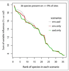
(32) 7.3. RESULTS. 7.3.1 Prediction of species occurrence using environmental explanatory variables The 36 species that occurred on at least nine percent of the 366 BRUVS sites were used in an analysis of univariate and multivariate boosted regression trees (BRT) to predict the probability of occurrence (0 to 1) of a species at a site using all 28 spatial and environmental covariates as predictors (Table 7.1), and subsets made up of only the three spatial predictors and only the 25 environmental predictors. The performance of the three scenarios was assessed by comparing the summed influence of the predictor variables (%var.infl) both as an average across all 36 species, and separately for each species. Species such as Gymnocranius audleyi in Table 7.1 with low ‘%var.infl’ were the least predictable. For that particular species, the errors reported in Table 7.1 hide the fact that presence (as distinct from absence) was predicted successfully, on average, for only one of the 34 BRUVS sites on which this species was recorded. The classification error did not distinguish between false negatives and false positives. I compared BRT models using, (a) all 28 spatial and environmental variables (mean %var.infl =13.2%); (b) using only the spatial variables ‘across’, ‘along’ and depth (mean %var.infl =12.9%); and (c) using environmental covariates only (mean %var.infl =13.05%). The differences amongst the scenarios were visualised by ranking the summed influences of the predictors (%var.infl) in univariate BRT from the first, most predictable, species to the least at rank number 36, and plotting them together in Figure 7.1. The differences were most evident for the first fourteen most predictable species in each scenario (Figure 7.1). These top ranked species were different in each scenario. The simple model containing only spatial position ‘across’ and ‘along’, and depth, performed reasonably well, but use of the 25 environmental covariates was better. Performance converged for lower ranked species. The mean variance in the species responses explained by the full BRT model was 83% and the average relative prediction error was 16.9%.. 173.

(33) Table 7.1. Results of the univariate and multivariate BRT for the 36 most prevalent species (y) at n=366 sites using all 28 explanatory variables (x). The species were present at ‘occ’ sites, and ‘sdt’ was the number of correct predictions, on average, over 1,000 univariate BRT with five-fold cross-validation. Relative prediction error was ‘rel.PE’ = (1 –(sdt/n))%, and the percentage of the variation in occurrence of each species explained by the best gbm model was ‘%Var’. The species were ranked in decreasing order of their average ‘predictability’, represented by the summed, average influence of all 28 predictor variables (‘%var.infl‘).. Species. occ. sdt. rel.PE. %Var. %var.infl. Scomberomorus queenslandicus. 167. 298. 18.6. 81.4. 19.9. Nemipterus theodorei. 127. 305. 16.7. 83.3. 18.8. Selaroides leptolepis. 128. 301. 17.8. 82.2. 18.7. Nemipterus furcosus. 192. 273. 25.4. 74.6. 18.7. Seriolina nigrofasciata. 155. 279. 23.8. 76.2. 18.5. Pentapodus paradiseus. 135. 289. 21. 79. 18.3. Abalistes stellatus. 147. 275. 24.9. 75.1. 17.9. Pentapodus nagasakiensis. 103. 310. 15.3. 84.7. 17.1. Saurida_grp. 111. 284. 22.4. 77.6. 16.3. Nemipterus hexodon. 80. 337. 7.9. 92.1. 15.9. Echeneis naucrates. 171. 235. 35.8. 64.2. 15.7. Lethrinus genivittatus. 92. 297. 18.9. 81.1. 15.6. Lagocephalus sceleratus. 123. 256. 30.1. 69.9. 15.5. Carangoides coeruleopinnatus. 116. 260. 29. 71. 15.4. Decapterus russelli. 98. 278. 24. 76. 14.9. Gymnothorax minor. 81. 303. 17.2. 82.8. 14.4. Carangoides fulvoguttatus. 100. 264. 27.9. 72.1. 14.2. Upeneus tragula_grp. 85. 292. 20.2. 79.8. 14. Paramonacanthus otisensis. 67. 328. 10.4. 89.6. 13.3. Choerodon venustus. 64. 323. 11.8. 88.3. 12.8. Carangoides gymnostethus. 70. 296. 19.1. 80.9. 12.5. Parapercis nebulosa_grp. 69. 300. 18. 82. 12.4. 174.

(34) Species. occ. sdt. rel.PE. %Var. %var.infl. Gnathanodon speciosus. 52. 314. 14.2. 85.8. 10.5. Alepes apercna. 51. 318. 13.1. 86.9. 10.3. Nemipterus peronii. 48. 317. 13.4. 86.6. 9.9. Feroxodon multistriatus. 45. 321. 12.3. 87.7. 9.5. Pristotis obtusirostris. 44. 322. 12. 88. 9.3. Rhynchobatus djiddensis. 40. 326. 10.9. 89.1. 8.7. Lutjanus sebae. 40. 327. 10.7. 89.3. 8.6. Symphorus nematophorus. 40. 324. 11.5. 88.5. 8.6. Paramonacanthus filicauda. 37. 340. 7.1. 92.9. 8.5. Atule mate. 38. 335. 8.5. 91.5. 8.5. Scolopsis taeniopterus. 36. 331. 9.6. 90.4. 8.1. Carangoides hedlandensis. 36. 327. 10.7. 89.3. 8. Gymnocranius audleyi. 34. 331. 9.6. 90.4. 7.6. Lagocephalus lunaris. 34. 330. 9.8. 90.2. 7.6. 16.9. 83.1. 13.2. Means. 175.

(35) Figure 7.1. The performance of three scenarios of covariate selection in predicting the occurrence of vertebrate species in the GBRMP. The heuristic variables “across”, “along” and depth (aad), and 25 mechanistic, environmental variables (env) were analysed together and separately in the three scenarios. The top 36 species present on at least nine percent of sites were selected for plotting, and these were not necessarily ranked in the same order by prediction success for each scenario. The Y axes show the sum of average influences of explanatory variables (%var.infl in Table 7.1) from the cross-validated gbm models for each species in each scenario. A mixture of spatial and environmental covariates produced the optimal predictions (grey line), but use of position and depth alone produced reasonable prediction success (green line).. 176.

(36) The most predictable species were mainly small to medium sized (<300mm) nemipterids, carangids, lethrinids, monacanthids and labrids. However, larger-bodied pelagic piscivores (Scomberomorus queenslandicus) and omnivores (Lagocephalus) were also represented in Table 7.1. Predictability was generally greater for the more prevalent species in the dataset. The average influence of each of the predictors is ranked in decreasing order of importance in Table 7.2. Across-shelf and along-shelf gradients in sediment composition, seafloor topographic complexity, temperature, salinity, and seafloor current shear stress were most important, followed by epibenthic cover of marine plants and the amount of bare, or bioturbated, seafloor along video transects. Further down the list were variables relating to the epibenthic cover of ‘megabenthos’ and other covariates that were out-competed by surrogates. Some of these surrogates were both complementary and more comprehensive. For example, analysis of stills frames was available for only 332 of the 366 BRUVS sites, whereas towed video transect analysis was available for 342 sites. Given the stills camera was recording photographs in the same field of view as the towed video camera, the video records of the substrata and epibenthos were performing as better predictors than some of the still-frame covariates in the multivariate BRT models. A separate multivariate BRT model using the video records to predict the covariates recorded from the analysis of stills camera frames showed that the video surrogates (‘vid’ suffixes) predicted an average of about 28% of the variation in the eight covariates measured on still frames (‘pho’ suffixes). Four of these still-frame covariates at the bottom of Table 7.2 were predicted much better than this average (mgbnths.pc.pho 33.7%; othranim.pc.pho 26.1%; rugosity.pho.av 47.0%; rugosity.pho.sprd 55.5%), supporting the notion that their relative influence was downplayed by the presence of more comprehensive surrogates from the video analysis.. 177.

(37) Table 7.2. The 28 explanatory variables (x) sorted by descending order of the average influence of each explanatory variable (%var.infl) across all the 36 responses (species occurrences). In combination, these 28 covariates accounted for 83.1% of the prediction success and 86.8% of the variation for the 36 species in Table 7.1. The column rel.var.infl% expressed this average influence as a percentage of the grand average %var.infl = 13.2 in Table 7.1. Variable names were defined in Table 5.1.. Variable. %var.infl. rel.var.infl%. Variable. %var.infl. rel.var.infl%. across. 1.13. 8.54. gravl.pc. 0.46. 3.47. carbnte.pc. 0.74. 5.59. Temp.sd. 0.42. 3.17. depth. 0.67. 5.06. bioturb.pc.pho. 0.41. 3.10. rugosity.vid.av. 0.67. 5.06. bare.pc.vid. 0.41. 3.10. along. 0.62. 4.68. sand.pc. 0.37. 2.79. mud.pc. 0.59. 4.46. mgbnths.pc.vid. 0.37. 2.79. coarsns.pc. 0.58. 4.38. mgbnths.pc.pho. 0.37. 2.79. Salin.av. 0.58. 4.38. algae.pc.pho. 0.35. 2.64. Temp.av. 0.54. 4.08. othranim.pc.pho. 0.29. 2.19. dist.reef. 0.53. 4.00. bioturb.pc.vid. 0.29. 2.19. m.bstrs. 0.52. 3.93. rugosity.vid.sprd. 0.27. 2.04. Salin.sd. 0.52. 3.93. rugosity.pho.av. 0.23. 1.73. plant.pc.vid. 0.49. 3.70. rugosity.pho.sprd. 0.19. 1.43. nobiota.pc.pho. 0.46. 3.47. seagr.pc.pho. 0.15. 1.13. 178.

No results found