Constitutive model for large strain deformation of semicrystalline polymers

Semicrystalline Polymers

D. W. Holmes ([email protected]), J. G. Loughran and H. Suehrcke

School of Engineering, James Cook University, Townsville,Australia

May 15, 2007

Abstract. A constitutive model for large strain deformation of semicrystalline polymers has been formulated to predict the complex elasto-viscoelastic-viscoplastic material response. The general form of this model can be represented by three parallel rheological components corresponding to each of the modes of deforma-tion. It will be shown that such a configuration is well suited to the mechanical nature of polymers as observed in recent studies. The constitutive stress-strain-time relationships are drawn from continuum mechanics which are more suitable than simple linear expressions from rheology. The result is a large strain, fully three-dimensional constitutive model, derived from a thermodynamic basis. The proposed model can be fit to macroscopic experimental data and is highly suited to numerical analysis. The paper reviews the literature relevant to constitutive representation of semicrystalline polymers, provides conclusion and validation of the most suitable form of constitutive model and presents the relevant constitutive mathematics.

Keywords:Elasto-viscoelastic-viscoplastic, Semicrystalline Polymers, Constitutive Mathematics, Rheological Model

1. Introduction

Semicrystalline polymers are used widely in the manufacturing indus-try. Their ease of moulding and ability to be recycled makes them a very attractive material to use in a multitude of different applications, including in more recent years, where high or structural loading is expected during service. When high loads and elevated temperatures are involved it becomes increasingly important to be able to predict the loaded response of a material so as to allow confidence in service life and informed design choice. A constitutive model is a tool for such prediction and research to find an accurate constitutive model to represent semicrystalline polymers has been documented over many years by many authors.

As will be reviewed in the sections to follow, many different types of constitutive models have been proposed for application to semicrys-talline polymers with varying degrees of accuracy over a variety of

different loading circumstances. To date, however, there is still no one model that is generally accepted to perform satisfactorily over a practi-cal range of loading circumstances. This is mainly due to the complexity of the response under load of the material. As will be shown, semicrys-talline polymer response comprises certain degrees of time variant and invariant response and it is the accurate account of these that has been the aim of the majority of previously proposed constitutive models. It could be argued that for the general case, this goal is yet to be achieved. This paper partly acts to review literature associated with the de-velopment of a constitutive model for semicrystalline polymers and to collate the resulting requirements of such a model so as to allow informed selection. This paper then uses this review to justify the selection of a continuum mechanics model that has not previously been suggested for semicrystalline polymers. This model is theoretically compared with experimental testing on semicrystalline polymers from the literature as means of validation.

Section2provides background on constitutive modeling, specifically rheological models. In Section 3, a review of literature relevant to the aims of this paper is carried out, concluding on the requirements of a suitable model for semicrystalline polymers based on the reviewed literature. A new model is then proposed. Section 4 presents the val-idation of the chosen model based on theoretical comparison between model capabilities and experimental test results from the literature. The constitutive mathematics that accompany the chosen model are collated in Section 5.

2. Background

In continuum mechanics there are various forms of constitutive theo-ries that can be used for representation of the deformation behavior of materials. Peri´c and Owen [48] outline two major model types as micromechanical models and phenomenological models. Micromechan-ical models predict material response by simulating interactions on a molecular level. Phenomenological theories rely on macroscopic obser-vations of representative volumes of material. Peri´c and Owen make note that the most powerful phenomenological theories should still take into account the “. . . underlying microscopic dissipation mechanisms”

Rheological models are an effective tool for understanding and rep-resenting the mechanical properties of a material. By combining simple elements such as springs and dashpots, a complicated material response to loading can be represented by a combination of easily visualized simple responses. In this form a rheological model constitutes a consti-tutive theory. In deformation analysis, rheological consticonsti-tutive theories are widely used for two main purposes. The first of these is as a concep-tual aid to help visualize the way in which a material behaves during deformation. An example of this would be to visualize the behavior of a spring when trying to understand elastic material behavior. The second is as a quantitative tool for use in predicting the loaded response of a material either manually or numerically in the form of a finite element simulation. The second of these is more pertinent to our endeavor.

When used in the form of a quantitative constitutive theory, rheo-logical models provide the framework to which controlling constitutive mathematics are applied. Such mathematics can be either derived from the linear component expressions such as Hooke’s laws in the case of a spring or from analogous but more complicated, nonlinear theories. Such nonlinear theories can take direction from micromechanical dissi-pation (Peri´c and Owen [48]). Where the linear constitutive expressions allow simplicity of formulation and implementation, the nonlinear the-ories allow for, in many cases, a more realistic representation of loaded responses where complicated load and rate dependencies are involved. The constitutive mathematics dictate the relationships between stress and strain as well as other parameters including strain-rate, time, temperature and material variables for each rheological component.

The configuration of a rheological model governs the interrelation-ships between each element. Different positioning of springs, dashpots, etc. in a rheological model can result in very different model responses to deformation. The presence and timing of required forms of deforma-tion can be controlled by the suitable selecdeforma-tion of model configuradeforma-tion. It is equally important to have both a well constructed rheological framework and plausible constitutive mathematics.

3. Review of Literature

Given the shear volume of published research on the constitutive be-havior of semicrystalline polymers, within the current investigation it would seem impractical to provide a comprehensive review of the litera-ture. Rather, it is the aim here to enable conclusion on the requirements of a general model for semicrystalline polymers and to report on a representative cross-section of constitutive model types that have been used to date. The survey allows informed specification of the most appropriate model for this type of material.

3.1. Direction from micromechanics

The molecular deformation mechanisms treated by micromechanical constitutive theories are generally measured explicitly during observa-tion on molecular interacobserva-tions using techniques like X-ray scattering [18]. Such testing is significantly more definitive in regards to measur-ing the actual modes of deformation present (elasticity, viscoelasticity, etc) than the global stress-deformation measurement techniques used in macroscopic research. Correspondingly, while not the primary fo-cus of this investigation, a brief review of micromechanics would seem beneficial.

Firstly, it is important to note that semicrystalline polymers are characterized by a morphology of crystalline regions of ordered lamel-lae, surrounded by amorphous regions of unordered molecular chains. The amorphous regions in close proximity to, or between crystalline lamellae are noted to have greatly reduced mobility and are often re-garded as a third region [5,10,11]. It is the interactions and behavior of these structures that account for the complex deformation behavior of semicrystalline polymers.

It is widely accepted that on the molecular level, deformation of the semicrystalline structure results from a combination of elastic, vis-coelastic and viscoplastic modes (see for example [11,12,14]). Elasticity is associated with the stretching of molecular chains within the amor-phous phase [5,18]. A mechanism that can be compared to the behavior of purely hyperelastic materials such as rubbers and elastomers [40]. Drozdov and co workers [10, 11, 12, 13] conclude that viscoelastic response is the result of molecular chain rearrangement within the amorphous phase; primarily, the separation of chains from lamellae junctions and connection of free chains with new junctions. Thermal activation is thought responsible for these rearrangements where an increase in a molecules energy enables its jump to a higher state [10]. The concept of viscoelastic recovery is then viewed as the progres-sive return of the molecular chains to their original state upon the removal of energy from the system (i.e. unloading). Viscoplastic defor-mation has been observed by Schrauwen et al. [57] and also Drozdov and Christiansen [12] to initiate in the amorphous region via inter-chain slippage1_{. At higher strains, this transitions into the crystalline} phase where fine, and then coarse lamellae sliding occurs with eventual fragmentation of the crystallites.

An explicit yield threshold is commonly observed at small strain lev-els (for exampleε= 0.02 [11]) far before necking. Schrauwen et al. [57] have also observed additional yielding phenomena for strains in excess of necking (up to 200% strain). The actual mechanisms of yield are noted to be the source of some conjecture [11], however generally, yield results from the increased load on molecular chains (most significant in the crystalline phase [57]), where some required threshold of thermody-namic potential is reached so as to allow slippage of chain-chain bonds. Strain hardening is also commonly observed. G’Sell et al. [18] explains such phenomena to be primarily the result of lamellae fragmentation that corresponds to an increase in the restricted amorphous phase. This phase reinforces the remaining lamellae fragments and so limits further

1

viscoplasticity. The chain density in the amorphous phase before and after deformation plays a key role in this phenomena [57].

A fully general macroscopic model should account for all the defor-mation mechanisms observed within the microstructure, as summarized here.

3.2. Macroscopic constitutive theories

The review that follows is concerned mainly with large strain consti-tutive models for semicrystalline polymers. Based on the conclusions from the preceding section, our attention will be limited to models that account for some amount of elastic, viscous and plastic deformation.

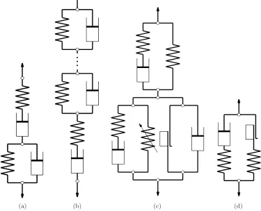
Findley et al. [17], while largely concerned with nonlinear viscoelas-tic integral theories, presents a simple elasto-viscoelasviscoelas-tic-viscoplasviscoelas-tic rheological model termed the Burgers model (Figure1 (a)). While the Burgers model can reproduce the trends of some polymer experimental curves, it has been discounted mainly due to the fact that polymer viscous and plastic responses are known to be nonlinear for all cases other than for small strain. Findley et al. [17] summarized a shift from the use of conventional rheological models due to their restriction of linearity. Modern rheological models can be used as framework for nonlinear theories, however the other limitation to the Burgers model is its lack of expression for an actual yield threshold with irrecoverable deformation being present at all stages of loading.

(a) (b) (c) (d)

Figure 1. One-dimensional elasto-viscoelastic-viscoplastic rheological models used for semicrystalline polymers by (a) Findley et al. [17], (b) Schapery [55], (c) Brusselle-Dupend et al. [5,6] and (d) Kletschkowski et al. [34].

over a variety of different loading cases and was shown to reproduce the experimental results well for all tested cases of positive strain, well into the necking region. The model was shown in all cases, however, to be inaccurate during unloading.

Lai and Bakker [36] propose an elasto-viscoelastic-plastic integral form constitutive theory for high density polyethylene. Total strain is additively decomposed into viscoelastic and plastic components and the constitutive theory is fulfilled using data from creep and recovery tests. The theory is shown to be accurate for simulation of various creep, recovery and constant stress rate loading and unloading. Again the model is phenomenological in nature but has little to do with actual molecular behavior.

are largely theoretical the first is written with the aim of representing fibre reinforced and un-reinforced plastics while the second is more generally noted to apply to several materials including semicrystalline polymers. Schapery’s model is based on the theoretical rheological framework shown in Figure 1(b). This model is similar to the Burgers model shown in Figure 1 (a) however it makes provision for any num-ber of viscoelastic components as may be required and accounts for all constitutive relationships in a nonlinear fashion. These component constitutive relations are based on thermodynamics rather than linear rheology. Schapery discusses theories to incorporate various additional nonlinearities, as well as other possible viscoplastic theories that may also incorporate yield.

Zhang and Moore [64,65] report on the elasto-viscoelastic-viscoplastic behavior of high density polyethylene pipes across constant strain rate, transient strain rate, single and cyclic loading-unloading, creep, relax-ation and combinrelax-ation tests. They then propose a nonlinear elasto-viscoelastic model derived from nonlinear rheology and an elasto-viscoplastic model derived from works by Bodner and Partom [1,2] on steel, to rep-resent observations. Both are uniaxial theories and the elasto-viscoplastic model assumes viscoplastic deformation to occur at all times and thus no yield expression is required. The two theories were compared against experimental results. It was observed that the elasto-viscoplastic theory was the superior of the two, closely predicting the majority of results seen experimentally. The nonlinear viscoelastic model was shown to be weak in predicting rapid changes in applied strain or strain rate while the only weakness with the elasto-viscoplastic model was its inability to predict strain reversal. While it would seem each of the tested models have certain advantages, it could be concluded that a more generally applicable model would incorporate both components of viscoelasticity and viscoplasticity. Other limitations with the models include the uniaxial restriction and the lack of expression for actual yield threshold or hardening in the elasto-viscoplastic model.

isotropic hardening and account for this in the rheological framework of the viscoplastic element. During tests at low strain, Brusselle-Dupend et al. also report a transitional zone between purely elasto-viscoelastic response and elasto-viscoelastic-viscoplastic response to occur at ap-proximately 1.5 _± 0.3 % strain. Thus the material was seen to have a definite viscoplastic yield point which was also accounted for in the model.

The viscosity of semicrystalline polymers (dash pot coefficients, Fig-ure1(c)) have been shown by Eyring [16] and later Halsey et al. [29] to evolve with varying inelastic strain rate (the Eyring model). Brusselle-Dupend et al. [5,6] found in experimentation that the Eyring model for evolution of viscosity, for each of the viscoelastic and viscoplastic flows was inadequate and so new expressions were formulated with added dependencies on total strain rate. The new viscosity expressions were shown by comparison to be highly superior to the polymer viscosity models used previously.

Constitutive model validation for the Brusselle-Dupend model was carried out by comparison with experimental data and it was shown that the simulations closely reproduced the expected results for mul-tiple cases of loading including combinations of loading, unloading, relaxation and recovery for several cases of strain rate. The work of Brusselle-Dupend and co-workers makes one of the most comprehensive attempts at accounting for the many mechanisms of semicrystalline polymers during deformation. While their model proved accurate across all cases published, there are still some important limitations. The rheo-logical configuration is relatively complex especially the representation of strain hardening. The formulation of the model is largely phenomeno-logical and, while accurate in application, it takes no direction from actual thermodynamics of the material continuum. Finally one of the more major limitations is that the theory is formulated for uniaxial application and would require significant work to extend the theory to account for three-dimensions.

de-formation is know to occur simultaneously, however Kletschkowski’s model accounts for these modes sequentially and so can be deemed to be questionable for the general case.

Peri´c and Dettmer [46] presented a finite strain constitutive theory generally applicable to most types of materials. Their model encom-passes any combination of elastic, viscoelastic, elasto-plastic or vis-coplastic response. Simultaneous account of these deformation modes is made possible by the parallel rheological framework on which the model is based. The generalized one-dimensional rheological representation is shown in Figure 2. The accompanying constitutive mathematics are derived from thermodynamics, allowing for both plastic and viscoplas-tic yield. Isotropic hardening is touched on and it is possible to extend the theory to account for kinematic hardening also, following references such as Simo [61]. The technique of using continuum mechanics the-ories implemented over a rheological framework has found wide prior application in specific forms for large strain deformation of inelastic materials (mainly rubbers and steels) as in works by Simo [58, 59], Simo and Hughes [60,61], Peri´c and Owen [47,48], Reese and Govind-jee [52] and Rosati and Valoroso [53]. Peri´c and Dettmer show that in a very general sense a model of this type can be widely generalized via the parallel combination of all the different types of possible elements (elastic, viscoelastic, viscoplastic and elasto-plastic). Peri´c and Dettmer demonstrate the models versatility by presenting numerical simulations completed using elasto-viscoelastic and elasto-viscoelastic-plastic forms of the model, each sited as representing the response of various types of rubber2_.

The works of Nedjar [38,39] deal with the formulation and numerical implementation of two large strain continuum mechanics type theories for application to filled rubbers, polymers and polymeric foams. The two different formulations are presented together and compared. The first model is based on a parallel combination of viscoelastic and vis-coplastic rheological elements identical to a reduced form of the Peri´c and Dettmer model, Figure 2. The second model is based on a series rheological addition of viscoelastic and viscoplastic components, similar to that used by Brusselle-Dupend et al. shown in Figure 1 (c). Like the work of Peri´c and Dettmer, both Nedjar’s models are formulated for three-dimensional, large strain with constitutive mathematics devel-oped from thermodynamics. Again, only linear viscosities are used. The second series model treated, involves no account of strain hardening and it would seem from the work presented that such a configuration is inappropriate for our purposes from both a response and

implemen-2

Figure 2. Generalized one-dimensional rheological representation of the elasto-vis-coelastic-plastic-viscoplastic Peri´c and Dettmer [46] model.

tation stand point. The firstparallel model, however, does incorporate isotropic hardening (and as before, kinematic hardening could be in-cluded with some development) and would seem an attractive model for semicrystalline polymers. A downfall of the specific model of Nedjar is, however, the lack of a wholly elastic component of response as was in-cluded in the Peri´c and Dettmer form. It will become evident in Section 4, that such an element is important for the response profiles observed during unloading and recovery, as observed by Brusselle-Dupend et al. [5,6] and so a reduced form of the model of Peri´c and Dettmer would seem the more appropriate choice as will be further discussed in the next section.

3.3. Model selection

It has only been in the last few decades that the technology has been available to allow microscopic deformation analysis. The great majority of macroscopic constitutive theories (dating back to the 1960s) were for-mulated based solely on experimental observation and phenomenology, thus limiting the ability to independently distinguish actual deforma-tion modes. This perhaps explains the length of time it has taken for this type of research to come to the conclusions that were confirmed so comparatively quickly by micromechanics.

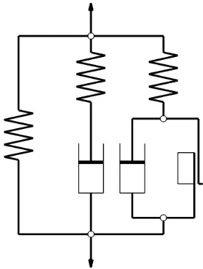
Figure 3. One-dimensional elasto-viscoelastic-viscoplastic rheological model.

with viscoplastic yield and strain hardening, have all been confirmed at macroscopic scale. In addition, macroscopic strain hardening has been observed to occur via both isotropic and kinematic mechanisms [5, 6, 18, 19, 22, 57] while a significant strain rate dependence of both the viscoelastic and viscoplastic viscosities has been observed [5,6,16,29]. No one existing model accounts for all these required behaviors and so an appropriate combination of components from existing theories will be used.

Based on the required deforming characteristics, we propose that a modified elasto-viscoelastic-viscoplastic form of the Peri´c and Dettmer model (Figure 3) be used, incorporating both isotropic and kinematic hardening as well as nonlinear viscosity expressions comparable to those presented by Eyring [16] and Brusselle-Dupend et al. [5,6].

A major advantage of this type of model is associated with the origins of the constitutive mathematics. While not explicitly modeling the micromechanics of deformation, continuum mechanics theories such as this are based on thermodynamic laws that represent the global effect of molecular interactions. Thus, direct analogy between such theories and the mechanisms discussed in Section 3.1is possible.

Firstly, hyperelastic theory is used for the elastic element where the energy of deformation is related to the thermodynamic system free energy in a similar way to that used in the micromechanical theories [11]. For viscoelasticity, viscous evolution is related to thermodynamic dissipation3 _{and is initiated and driven via interaction with another}

3

hyperelastic element, as would be the case on the molecular level. The viscoplastic evolution is also related to thermodynamic dissipation and is initiated by loading originating from elasticity. Isotropic and kinematic hardening are included which represent the fragmentation and subsequent fibril reinforcing of crystalline lamellae. For deforma-tion levels up to necking, a single yield point (well below the onset of necking) represents where microscopic yielding mechanisms become macroscopically evident.

The intimate relationship between macroscopic representation and the actual microscopic deformation mechanisms, further reinforces the value of a model such as this.

4. The Suitability of the Selected Rheological Form to Polymers

While the chosen Peri´c and Dettmer parallel model configuration (Fig-ure3) is desirable from a numerical standpoint, its explicit applicability to semicrystalline polymer response is yet to be confirmed. As a pre-liminary assessment for the performance of the parallel rheological configuration, one-dimensional, linear constitutive mathematic from rheology were used4_{. Hooke’s law was used for the elastic element(s)} [17]

σe=Eeε (4.1)

and a simple newtonian evolution expression was used for the viscoelas-tic element [17]

σve=Eve

ε₋εi_ve, ε˙i_ve = 1

ηve

σve (4.2)

Further a one-dimensional form of the Perzyna model equations were used for viscoplasticity (refer to Appendix Bfor further details)

σvp=Evp

ε₋εi_vp, ε˙i_vp= hfi

ηvp

∂f ∂σvp

f =_|σvp| −σy (4.3)

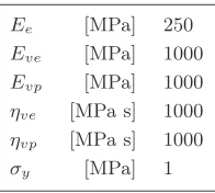
The material parameters were chosen arbitrarily and are presented for completeness in Table I.

The viscoelastic and viscoplastic evolution equations were solved using a Newton iteration scheme, analogous to that presented by Reese

4

Table I. Arbitrarily cho-sen 1D linear model pa-rameters

Ee [MPa] 250

Eve [MPa] 1000

Evp [MPa] 1000

ηve [MPa s] 1000

ηvp [MPa s] 1000

σy [MPa] 1

and Govindjee [52]. A simple strain controlled computational imple-mentation was used to generate the data presented in what follows. By showing that the parallel configuration is capable of reproducing the same deformation characteristics observed in the literature, the configuration is proven valid for these purposes.

4.1. Static Loading

Some of the earliest tests on the time dependent nature of polymers were static creep-recovery tests; Onaran and Findley [42], Lifshitz and Kolsky [37] and others as summarized by Findley et al. [17]. These tests involved maintaining a constant stress on a test sample and ob-serving the deformation response. Load removal then results in elastic and some degree of time dependent strain recovery. This observed de-formation response can be effectively reproduced by the 3 element, elasto-viscoelastic-viscoplastic model (Figure 3). During loading the applied stress is distributed through the three elastic springs with the viscoelastic and viscoplastic component springs driving time dependent deformation in the corresponding dashpots (providing spring stress exceeds that of yield in the case of the viscoplastic element). When an applied stress is held constant the evolution of the viscoelastic and viscoplastic dashpots proceeds while their element stresses de-crease to zero and below yield respectively while the elastic element stress increases to compensate and maintain a constant total load. The increasing elastic element stress necessitates an increase in total deformation and this time dependent strain increase is referred to as

is reached. This property effectively reproduces the phenomenon of plastic residual strain being present in polymer samples following long term creep testing at stresses far below the expected yield (Findley et al. [17]).

Release of the load results in a total model stress of zero, however due to dashpot strains the most likely stress distribution in the springs is one of tension in the elastic element and a counteracting compression in the other two. This residual element stress is what drives the creep mechanism in reverse, referred to as recovery. While the viscoelastic element stress will proceed to zero, that in the viscoplastic element will stop when the element stress decreases below compressive yield stress. As such a residual strain remains in the model. These results are all comparable to those observed by Onaran and Findley [42], Lif-shitz and Kolsky [37] and Findley et al. [17] for actual experiments on semicrystalline polymers.

Strain control tests are a powerful type of test for formulating and testing a material with simultaneous modes of deformation such as is the case for semicrystalline polymers. Such testing simplifies the isolation of the parallel modes of deformation and has been used almost exclusively in more recent polymer testing. Relaxation testing is one of the earliest forms of this type of test. A relaxation test involves main-taining a constant strain on a test sample and observing the response to stress (Findley et al. [17]).

The response of the proposed model (Figure 3) during stress relax-ation can again be audited. The initial strain applicrelax-ation will result in a distribution of the total stress across the three element springs driving inelastic evolution in the case of the viscoelastic and viscoplastic ele-ments in a similar fashion as above. Upon hold of the level of strain, the elastic element stress will remain constant while that in the viscoelastic and viscoplastic elements will decrease with the progressive evolution of the dashpots. This progressive decrease in stress is referred to as

stress relaxation. Again the viscoelastic stress will approach zero while the stress in the viscoplastic element will become constant when the spring stress becomes less than that of yield. Once again this type of response is exactly as would be expected for a semicrystalline polymer as reported by Findley et al. [17].

4.2. Constant Strain Rate Loading

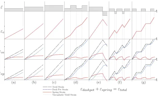
Figure 4. Theoretical strain curves for the proposed elasto-viscoelastic-viscoplastic rheological model showing all element components of strain for (a, b and c) constant strain rate tests, (d) changing strain rate tests, (e) loading-unloading test, (f) cyclic loading-unloading test and (g) cyclic loading-relaxation test. Figures are not drawn to scale.

rheological model configuration. Four graphs are shown; the top is the magnitude of strain rate over time followed by component strain vs. time response for the elastic, viscoelastic and viscoplastic elements respectively. The strain vs. time graphs show the total element strain (all three elements have equal total strain), the component of strain in the element spring and the component of strain in the dashpot is as per the key shown. Spring and dashpot strain components are a decompo-sition of the total strain for each element. For the viscoplastic element response, a faint horizontal line shows the spring strain corresponding to the element yield stress.

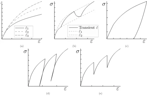
of three different strain rates applied to the same model. It can be observed that an increase in strain rate corresponds directly to an increase in each component’s level of spring strain and so total stress. Total model stress has been calculated and is plotted against total strain in Figure 5 (a) for these three strain rates. Authors such as G’Sell and Jonas [20,21], Kitagawa and colleagues [31,32,33], Popelar et al. [50], Duffo et al. [15], Zhang and Moore [64, 65] and Kontou and Farasoglou [35] have readily observed constant strain rate tensile test curves such as those in Figure 5(a). One such experimental curve set is shown in Figure 6 (a)5 _{for comparison (taken from Kitagawa} et al. [33]). Similarly shaped curves and similarly increasing levels of stress corresponding to the increasing strain rates are observed by all authors and can be likened to that seen here for the proposed elasto-viscoelastic-viscoplastic model.

Tests that are often carried out during polymer research involve constant strain rate tests with mid test transient jumps to different values of strain rate. A theoretical simulation of such a test has been carried out for the proposed rheological model in a similar fashion to the constant strain rate tests above. Figure 4(d) shows the theoretical test strain rate, elastic, viscoelastic and viscoplastic component strains against time. It can be observed that for all elements, modifications in strain rate affect all components of strain as if the difference in strain rate has been added to or subtracted from the existing response. It can also be observed that the spring strain for the viscoelastic and viscoplastic elements always approach the same equilibrium value for the same applied strain rate. Again, the total model stress response is shown against total strain in Figure 5 (b). The monotonic paths corresponding to each strain rate are superimposed on the figure. The observed path of the stress strain curve due to transient changes in strain rate and the apparent lack of history dependence on strain rate has been observed in experimental testing on semicrystalline polymers by G’Sell and Jonas [21], Kitagawa and Matsutani [31], Kitagawa et al. [32], Kitagawa and Takagi [33] and Zhang and Moore [64,65]. Ex-perimental results from Zhang and Moore [64] are shown in Figure 6 (b) for comparison.

Other types of tests using changing states of constant strain rate have also been used in the evaluation of polymer constitutive models. Kitagawa and Matsutani [31], Popelar et al. [50], Zhang and Moore [64, 65], Pegoretti et al. [44], and Brusselle-Dupend et al. [5,6] have all con-ducted loading-unloading tests where both the loading and unloading

5

(a) (b) (c)

(d) (e)

Figure 5. Theoretical total stress vs. total strain curves for the proposed elasto-vis-coelastic-viscoplastic rheological model for (a) three constant strain rate tests, (b) changing strain rate test, (c) loading-unloading test, (d) cyclic loading-unloading test and (e) cyclic loading-relaxation test. Figures are not drawn to any scale.

(a) (b) (c)

(d) (e)

Figure 6. Experimental total stress vs. total strain curves taken from the literature for (a) constant strain rate tests, Kitagawa et al. [33]: Figure 4, p 1947, (b) changing strain rate test, Zhang and Moore [64]: Figure 3, p 407,(c) loading-unloading test, Brusselle-Dupend et al. [6]: Figure 13, p 512, (d) cyclic loading-unloading test, Zhang and Moore [64]: Figure 5, p 407 and (e) cyclic loading-relaxation test, G’Sell and Jonas [21]: Figure 7, p 1962 (shown to∼0.75 strain).

the authors referenced above, an example of which is provided from Zhang and Moore [64] in Figure6(d) for polyethylene. Another point of comparison is that the point of stress reached by consecutive unloadings increases with each unloading instance observed in both Figure 5 (d) and Figure 6(d).

Another form of cyclic test that is used during testing on semicrys-talline polymers is cyclic loading-relaxation. This test loads the sample at a constant strain rate and then for a designated period of time, main-tains constant strain, observing the relaxation in stress. This portion of stress relaxation is exactly the same as has been discussed above in the static loading section except that the level of strain was reached by a ramp in strain rather than a simple transient step. Component strains for a theoretical simulation for this type of loading are shown in Figure4 (g). The relaxation periods are simply periods of zero strain rates as shown. The total model stress has been calculated and is shown against total strain in Figure 5 (e). Again upon reapplication of the load-ing, the stress-strain curve quickly approaches the path it would have traveled were there no unloading. Comparison for the initial loading-relaxation curve component can be made to that reported for PP by Brusselle-Dupend et al. [5,6]. The results for cyclic loading-relaxation simulations are also comparable to those found during testing by G’Sell and Jonas [21], Kitagawa and Matsutani [31] and Kitagawa et al. [32]. A figure for comparison with actual experimental result on HDPE is given in Figure 6 (e)6 _{from G’Sell and Jonas [21].}

4.3. Other Phenomena

Another property that polymers are known to exhibit is the full recov-ery of plastic deformation upon heat treatment. This full recovrecov-ery is reported to be possible after tests of up to 20% strain in semicrystalline polymers (Pegoretti et al. [44]) and up to 50% strain in amorphous polymers (Oleynik [41] and Quinson et al. [51]). Most importantly Pegoretti et al. [44] notes that the plastic deformation in semicrystalline poly(ethylene-terephthalate) or PET resulting from tests carried up to 20% strain at room temperature, can be fully recovered during a 6 min heat treatment at 160˚C. This temperature is approximately 45˚C higher than the materials glass transition temperature. The necking point of a polymer has long been know to be influenced by temperature (Brostow and Corneliussen [4] and Budinski and Budinski [7]) so it would be intuitive to predict that the actual viscoplastic yield would also be influenced in such a manner. With such an added dependency

6

the proposed model would also be capable of reproducing the plastic recovery observed by Pegoretti et al. [44].

With correct expression of the temperature dependency of the vis-coplastic yield stress in both tension and compression, the proposed model would be capable of total thermal plastic recovery. Referring to the earlier explanation, recovery is driven by non-zero residual el-ement spring stresses. Following load removal, the compression in the viscoelastic component drives a full recovery of deformation. The vis-coplastic element does not however recover because in most room tem-perature cases, the compressive yield of the material will be far greater than the residual compressive stress left in the viscoplastic component. Allowing a high enough temperature in the recovery stage to reduce the compressive yield stress toward zero would allow free compressive evolu-tion in the viscoplastic dashpot and thus recover just as the viscoelastic component does. Given enough time at the elevated temperature with compressive yield stress equal to zero, the model would fully recover as is observed by Pegoretti et al. [44] in real materials.

A noteworthy point is in regard to the contributions of stress relax-ation and strain recovery from the viscoelastic and viscoplastic compo-nents. Figure 4 (g) shows viscoplastic contribution to relaxation until the stress reduces below yield. In real materials it is noted that relax-ation is a property of viscoelasticity (Brusselle-Dupend et al. [5, 6]). This is one reason for the importance of kinematic and isotropic hard-ening in a model for semicrystalline polymers, properties not accounted for in the above linear study. Such hardening rules increase the yield limit with the highest level of stress reached. In this way upon the onset of a relaxation period, the viscoplastic element stress would im-mediately drop below the hardened value of yield and so no relaxation contribution will take place. This is also the case during load rever-sal and recovery meaning only elastic forms of deformation can be recovered as is expected. The absence of strain hardening in the lin-ear model presented here is the one discrepancy between the above curve responses and those observed in reality however this is taken into account in the more advanced constitutive mathematics to follow.

5. Formulation of Constitutive Mathematics

of isotropic and kinematic hardening suitable for the semicrystalline polymer case. The numerical implications of incorporating strain rate dependent viscosity expressions for a three-dimensional, large strain model will also be treated.

5.1. Kinematics and Thermodynamics

Let us first establish some of the kinematic and thermodynamic foun-dations that the theory will depend on.

Of particular importance to the measurement of finite deformation is the second order deformation gradient tensor, F [3]. A key charac-teristic of finite deformation is the presence of rigid body motion. A consequence of this is that some arbitrary vector within the continuum of a deforming body can be described either in terms of its position in space or relative to its initial material position. These are referred to asEulerian andLagrangian descriptions respectively. The deformation gradient describes the final spatial configuration of such a vector with respect to its initial material configuration. The deformation gradient is evidently associated with strain in both Lagrangian and Eulerian space, hence its importance to continuum mechanics.

Particularization of strain measurement into exclusive Lagrangian or Eulerian description results in the common measures of tensorial strain; C = FTF, the Lagrangian right Cauchy-Green strain tensor and b = F FT, the Eulerian left Cauchy-Green strain tensor. Spec-tral decomposition of these quantities enables the recovery of principal strain measures used widely in material science. This decomposition is treated at length by authors such as Bonet and Wood [3], Simo and Taylor [62] and Itskov [26,27,28] and proceeds

C = 3 X

A=1

ΛANA⊗NA b=

3 X

A=1

ΛAnA⊗nA (5.1)

where ΛA,A= 1,2,3 are the common eigenvalues ofCandbwhileNA andnAare the Lagrangian and Eulerian eigenvector triads respectively [3]. Correspondingly, λA =√ΛA are the principal stretches and εA =

ln(λA) are the logarithmic principal strains each commonly used in the experimental literature ([5,6], [20], [63] for example).

Figure 7. The multiplicative split of the deformation gradient into elastic and inelastic components.

is facilitated via the multiplicative split of the deformation gradient

F =FeFi (5.2)

This is diagrammatically represented in Figure 7. From the figure, where the total deformation gradient maps the initial configuration, A

to its deformed configuration C, it is conceptually equivalent to allow the elastic component Fe to map A to some intermediate position B

and correspondingly for the inelastic component Fi, to mapB to the final configuration C. From rearrangement of Equation5.2, it is conve-nient to establish the elastic components of right and left Cauchy-Green strain as

Ce=Fe TFe be=FeFe T (5.3)

Within continuum mechanics, a large part of the accurate expression of a materials constitutive behavior is associated with expression of the materials thermodynamic free energy, ψ. Referring to Reese and Govindjee [52], the expression of free energy can be given

ψ= ˆψ(C, ξ1, ξ2, ..., ξn) (5.4)

because the free energy is a continuum quantity, it must be defined in terms of Lagrangian strain7_.

The strain dependence of the free energy is commonly associated with elastic mechanisms [40] while the internal variables are generally associated with the inelastic response [46, 61] which gives rise to the decoupled expression treated by Peri´c [45]

ˆ

ψ(Ce, ξ1, ξ2, ..., ξn) = ˆW(Ce) + ˆH(ξ1, ξ2, ..., ξn) (5.5)

where ˆ_W is the elastic thermodynamic potential, examples of which include the St. Venant-Kirchhoff (elastic), and Ogden (hyperelastic) models [3], while the definition of ˆ_H clearly depends on the nature of the internal variables. Given that ˆψ is associated with material defor-mation that can be separated into elastic and inelastic components via Equation 5.2, then ˆ_W is only functional on the elastic component as shown [38, 52]. It follows that for a purely elastic material, Ce = C

such that

ˆ

ψ(C) = ˆ_W(C) (5.6)

where no internal variables are necessary.

Focusing on the particular case of an elasto-viscoelastic-viscoplastic constitutive theory, because of the parallel configuration (Figure 3), it is a common convention to define the total free energy expression via the sum of the components [23,24,38,52] as

ψ= ˆψe(C) + ˆψve(Ceve, ηve) + ˆψvp

Ce_vp, ηvp, α,α

(5.7)

whereαandαare viscoplastic internal variables associated with isotropic and kinematic hardening respectively, and also, contrary to the tradi-tional form of ˆψve and ˆψvp (for example [52,46] for viscoelasticity and [45, 46, 59, 61] for viscoplasticity), the viscosity terms ηve and ηvp have been included as additional internal variables. This is due to the requirement that the viscosity terms used in any constitutive model for semicrystalline polymers, have some functionality on strain (Section 3.3). We will elaborate further on this point in subsequent sections.

5.2. Stress

To allow definition of the constitutive stress expression, it is necessary to observe that, following for example Holzapfel [23], Nedjar [38] and Reese and Govindjee [52], all constitutive equations must satisfy the

7

2nd _{law of thermodynamics. In Lagrangian description, this can take} the form of the Clausius-Plank inequality8

S :1₂C˙ ₋ψ˙ _≥0 (5.8)

where S is the second Piola-Kirchhoff stress tensor. By the standard development [38,46,52,59], implementation of Equation5.7into Equa-tion 5.8 enables the explicit definition of the stress expression. This development is included in Appendix A.

From Appendix A, the total second Piola-Kirchhoff stress is given by

S = 2∂ψˆe

∂C + 2F

i₋1 ve

∂ψˆve

∂Ce_veF

i₋T

ve + 2Fivp−1

∂ψˆvp

∂Ce_vpF

i₋T vp

=Se+Sve+Svp (5.9)

In solid mechanics, while the account of the constitutive behavior of a material is inherently Lagrangian [3], it is convenient from an implementation standpoint, to also define the Eulerian quantities. Cor-respondingly, the Eulerian counterpart to S, is the Kirchhoff stress tensor τ. Lagrangian and Eulerian quantities are related through the concepts of push forward and pull back [3, 62] where the Kirchhoff stress can be attained from the second order push forward of S via

τ =F SFT (5.10)

Following Equation5.10, then Equation5.9 becomes

τ = 2F∂ψˆe

∂CF

T _{+ 2F}e ve

∂ψˆve

∂Ce_veF

e T

ve + 2Fevp

∂ψˆvp

∂Ce_vpF

e T vp

=τe+τve+τvp (5.11)

Because of the functionality ofτve andτvpon the elastic component of strain, it remains to define the evolution of inelastic strain9_.

5.3. Viscoelastic evolution equations

Limiting our attention to the evolution of the viscoelastic response, following from Appendix A, this must satisfy the inequality

τve :

−1 2(Lvb

e ve)beve−1

−∂ψˆve

∂ηve · ˙

ηve ≥0 (5.12)

8

also commonly referred to as the Clausius-Duhem inequality.

9

Note Ce _=Fi−T_{C F}i−1

such that, given the inelastic evolution, Ce _{can be}

The ₋∂ψˆve

∂ηve ·η˙ve term is associated with the evolution of the viscosity internal variable and will be treated subsequently. The remaining term is associated with strain evolution and is of primary interest.

Reese and Govindjee [52] introduce the expression

−₂1(_Lvbeve)bvee−1 :=V−1:τve (5.13)

where now the left hand side of Equation 5.12becomes

τ :_V−1 :τ _≥0 (5.14)

which is satisfied for all cases of τ providing _V−1 _{is positive definite.} The left hand term of Equation5.13is related to the rate of inelastic material strain through operator split theory. For the current investi-gation it is sufficient to draw the analogy between Equation 5.13 and Equation4.22of the infinitesimal 1D theory, where hereV−1 represents the inverse viscosity in fourth order tensor space.

An inverse viscosity term suitable for polymers has been proposed by Reese and Govindjee [52] as

V−1 = 1 2ηD

I′₄₋1₃I_⊗I+ 1 9ηV

I _⊗I (5.15)

whereηDandηV are deviatoric and volumetric components of viscosity respectively. The authors indicate that the viscosity terms ηD and ηV could be strain dependent but offer no further development. The terms (I′₄₋1₃I_⊗I) andI_⊗I operate through the double contraction withτve to isolate the deviatoric and volumetric components of stress respec-tively (Simo [59]). HereI₄′_ijkl = 1₂(δikδjl+δilδjk) is the supersymmetric 4th order identity tensor and Iij =δij is the 2nd order identity tensor (Bonet and Wood [3]). Holzapfel [23] notes that based on experimental results, the inelastic evolution of most polymeric materials is wholly deviatoric and consequently, the volumetric term from (5.15) can be ignored (i.e. ηve =ηD). This property is further confirmed in the works of Peri´c and Dettmer [46] and Reese and Govindjee [52].

It is left to establish the actual form of viscosity expression that would allow adequate account of the strain rate dependence observed for semicrystalline polymers.

In the context of one-dimensional, finite deformation, Brusselle-Dupend et al. [5, 6] have proposed a viscosity expression for the viscoelastic response of semicrystalline polypropylene as

ηve =

h0−h1exp n

h2|ε˙

e_|+3×10−5

|ε˙i_| o

−h3exp n

h4|ε˙

e_|+3×10−5

|ε˙i_| o

where h0,1,...,4 and ne are material constants. This equation was de-veloped due to the reported inadequacies with the conventionally used Eyring equation [16, 29] when applied to semicrystalline polymer re-sponse.

For three-dimensionality, the viscosity of a material remains a scalar quantity (as per Equation 5.15) however the multidimensional depen-dencies of this value have not been treated with any generality in the literature, particularly for the case at hand. As a consequence, it would appear that a significant amount of experimental work is needed to allow development of a three-dimensional analog to Equation 5.1610_.

Developing on this concept briefly, because of its strain dependence, the viscosity is considered to be an internal variable in a similar way to the strain hardening terms from plasticity. Following from Peri´c [48], Reese and Govindjee [52] and Simo and Hughes [61] it is most desirable to define the constitutive behavior of internal variables via their evolution, i.e.

˙

ηve= ˆηve

Ci_ve, ηve

= ˆηve

FTbe_ve−1F, ηve

(5.17)

By specifying the constitutive behavior of the viscosity in this way, a numerical solution scheme such asClosest point projection, convention-ally used in plasticity [45,61], can be used for the simultaneous solution of strain (Equation 5.13) and viscosity (Equation5.17). For the case of linear viscosity the viscoelastic constitutive theory can be implemented via a local Newton iteration scheme [52], a method like closest point projection can be interpreted as performing this Newton iteration for two or more mutually dependent variables.

An additional requirement of the constitutive behavior of the viscos-ity is that the evolution expression Equation 5.17, and the free energy component ˆ_Hve(ηve), must suitably satisfy the right hand side of the dissipation requirement, Equation 5.12.

5.4. Viscoplastic evolution equations

The derivation of the constitutive equations for one-dimensional vis-coplasticity with isotropic and kinematic hardening is presented for reference in Appendix B.

For three-dimensional large strain, as was the case for viscoelasticity, the viscoplastic constitutive equations must satisfy the thermodynamic

10

dissipation requirement (Appendix A)

τvp :

−12

Lvbevp

be_vp−1₋∂ψˆvp

∂ηvp · ˙

ηvp−

∂ψˆvp

∂α ·α˙− ∂ψˆvp

∂α : ˙α≥0 (5.18)

where again viscosity is implemented as a strain dependent internal variable and the scalar α and tensorialα internal variables are associ-ated with isotropic and kinematic hardening mechanisms respectively (akin to αiso and αkin from the one-dimensional theory).

It is again pertinent to introduce the stress space conjugates to the isotropic and kinematic hardening internal variables, namely q and q. By a similar argument to that which motivated the formulation of Equation 5.5, referring to Peri´c [45], Simo [59] and Simo and Hughes [61], the viscoplastic free energy can be expressed

ˆ

ψ(Ce_vp, ηvp, α,α) = ˆW(Cevp) + ˆHηvp(ηvp) + ˆHαvp(α) + ˆH α

vp(α) (5.19)

Implementing a combined, linear isotropic/kinematic hardening law following Hughes [25] and Simo and Hughes [61], it can be shown that

ˆ

Hαvp= 12θH¯α

2 _ˆ

Hα

vp= 12(1−θ) ¯Hα:α (5.20)

∂_Hˆα vp

∂α =θH¯α=−q

∂_Hˆα vp

∂α = (1−θ) ¯Hα=−q (5.21)

where ¯H is a constant parameter representing the combined hardening modulus andθdefines the proportions of isotropic and kinematic hard-ening; θ_∈[0,1]. It follows directly from Equation 5.21 that the actual

hardening moduli are given

−∂

2_Hˆα vp

∂α2 =−θH =¯

∂q

∂α −

∂2_Hˆα vp

∂α2 =−(1−θ) ¯HI⊗I =

∂q

∂α (5.22)

These constant terms are inferred to be suitable for the current pur-pose however for more complex hardening characteristics, alternate specification of ˆ_Hα

vp and ˆH α

vp can be used.

Given the stress space hardening internal variables, it is possible to carry out a three-dimensional study of the effects of strain hardening on the yield surface as was done for the one-dimensional case (Appendix B). Following Simo [59], Simo and Hughes [61] and Zienkiewicz and Taylor [66], selection of the von-Mises yield surface gives the yield function

f(τvp+q, q) =kτvp+qk − q

2

3(σY −q) (5.23)

Physically q2

3(σY −q) quantifies the radius of the yield surface, while

inelasticity to have only deviatoric components such that now

f(¯τvp+q, q) =kτ¯vp+qk − q

2

3(σY −q) (5.24)

where ¯τvp= dev[τvp] and now the internal variableq is wholly devia-toric such that tr[q] = 0.

Following a similar development as for the one-dimensional case in Appendix B, Perzyna [49] and subsequent authors such as Simo [59], Simo and Hughes [61], Peri´c and Owen [47], Peri´c and Dettmer [46] and Rosati and Valoroso [53] define the evolution expression

− 1

2

Lvbevp

be_vp−1 = hf(¯τvp+q, q)i 2ηvp

∂f(¯τvp+q, q)

∂τ¯vp

(5.25)

Once again, an analogy is evident between this inelastic evolution and that reported for the one-dimensional case in Appendix B.

Referring to the explicit formulations of Simo [59], Simo and Hughes [61] and Zienkiewicz and Taylor [66], the evolution of the strain space hardening internal variables in tensor space are subsequently defined

˙

α= hf(¯τvp+q, q)i 2ηvp

∂f(¯τvp+q, q)

∂q (5.26)

˙

α= hf(¯τvp+q, q)i 2ηvp

∂f(¯τvp+q, q)

∂q (5.27)

Returning our attention to the dissipation requirement, Equation 5.18, neglecting the viscosity term11_{, substitution of Equations 5.21,}

5.24, 5.25, 5.26and 5.27yields with some manipulation

(τvp+q) : h

f_i

2ηvp

(I′₄₋1₃I _⊗I)

kτvp+qk

: (τvp+q) +q· q

2 3

hf_i

2ηvp ≥

0 (5.28)

which is unconditionally satisfied given that from definition of the ramp function (Equation B.8), _{h·i ≥}0 and also from the known behavior of isotropic hardeningq _≥0.

The considerations regarding strain rate dependence of the viscosity for the viscoplastic case are identical in form to those presented in Section5.3for the viscoelastic case. Consequently, no further discussion is necessary within the current investigation.

Exact specification of the elastic thermodynamic potential terms, ˆ

We(C), ˆWve(Ceve) and ˆWve(Cevp), to be used within a constitutive the-ory for semicrystalline polymers is largely case specific. Generally any

11

elastic or hyperelastic form of thermodynamic potential could be chosen (see Bonet and Wood [3]). A suggestion would be to use hyperelastic Ogden potentials for the elastic (Simo and Taylor [62]) and viscoelastic (Reese and Govindjee [52]) elements and an elastic type St. Venant-Kirchhoff potential for the viscoplastic element (Simo [59]). The choice of free energy expression must be governed by experimental observation because it must represent the thermodynamic potential of the material. As such final selection of the exact free energy form requires response curves from physical tests. For a more detailed discussion of hyperelas-tic free energy expressions for numerical use see Simo and Taylor [62], Simo [59], Peri´c and Owen [47], Reese and Govindjee [52], Simo and Hughes [61] and Peri´c and Dettmer [46].

6. Conclusions

The aim of this article was to determine the most appropriate con-stitutive theory for semicrystalline polymers based on a review of the literature. From both a microscopic and macroscopic perspective, de-formation characteristics such as elasto-viscoelasto-viscoplasticity, yield point, isotropic and kinematic hardening and strain dependent viscosi-ties have all been shown to be of significant importance. A model has been proposed that accounts for all these complex characteristics.

A preliminary study has shown the parallel rheological configuration of the chosen model to be suitable across a wide range of complex defor-mation behaviors based on comparison with experimental observations from the literature. Specific validation of the selected nonlinear, contin-uum mechanics constitutive theory is largely dependent on the explicit generation of material specific parameters (to be published at a later date), however the accuracy of such theories for the representation of similar materials (rubbers, elastomers etc) has been well documented. The model’s constitutive mathematics are presented in their most general form with the objective of being broadly applicable to all semicrys-talline polymers.

Acknowledgements

Appendix

Appendix A. Derivation of the dissipation requirement

For a constant temperature process, the Clausius-Plank form of the 2nd law of thermodynamics is expressed in Lagrangian form via

S :1₂C˙ ₋ψ˙ _≥0 (A.1)

where ˙C is the time differential of the right Cauchy-Green strain ten-sor, : denotes the tensor double contraction (see Bonet and Wood [3]) and ˙ψ is the time derivative of the free energy expression. The free energy expression ψ is expressed in terms of elastic, viscoelastic and viscoplastic components as

ψ= ˆψe(C) + ˆψve(Ceve, ηve) + ˆψvp

Ce_vp, ηvp, α,α

(A.2)

Note here that for the semicrystalline polymer application, the viscos-ity terms ηve and ηvp have become internal variables because of their functionality on strain (rate). Recalling the definition C =FTF and the multiplicative split of the deformation gradient Equation 5.3, it is convenient to substitute the relationships

Ce_ve=Fi_ve−TCFi_ve−1 and Ce_vp=Fi_vp−TCFi_vp−1 (A.3)

such that now

ψ= ˆψe(C) + ˆψve

Fi_ve−TCFi_ve−1, ηve

+ ˆψvp

Fi_vp−TCFi_vp−1, ηvp, α,α

(A.4) Following Reese and Govindjee [52] and Nedjar [38], taking the chain rule differential of (A.4) with respect to time gives

˙

ψ= ∂ψˆe

∂C : ˙C+

∂ψˆve

∂Ce_ve :

∂Ce_ve

∂C : ˙C +

∂ψˆve

∂Ce_ve :

∂Ce_ve

∂Fi_ve : ˙F

i ve

+ ∂ψˆvp

∂Ce_vp :

∂Ce_vp

∂C : ˙C+

∂ψˆvp

∂Ce_vp :

∂Ce_vp

∂Fi_vp : ˙F

i vp

+ ∂ψˆve

∂ηve · ˙

ηve+

∂ψˆvp

∂ηvp · ˙

ηvp+

∂ψˆvp

∂α ·α˙ + ∂ψˆvp

∂α : ˙α (A.5)

Separately evaluating specific terms from within (A.5), for the ˙C

terms, where the subscriptn=ve, vp

∂ψˆn

∂Ce_n :

∂Ce_n

∂C : ˙C =

∂ψˆn

∂Ce_n :

∂Fi_n−TCFi_n−1

∂C : ˙C

= ∂ψˆn

∂Ce_n :F

i₋T

where from Itskov [26, 28] and Kintzel [30], the derivative of some second order tensorAij with respect to its self is given by∂Aij/∂Akl=

I4ijkl =δijδkl, the fourth order identity tensor. Also, a useful identity used by Reese and Govindjee [52] associated with the double tensor contraction is A:B=C−1AD−1:DBC. Correspondingly

= 2Fi_n−1∂ψˆn

∂Ce_nF

i₋T

n : 12C˙ (A.6)

For the ˙Fi_n terms

∂ψˆn

∂Ce_n :

∂Ce_n

∂Fi_n : ˙F

i n=

∂ψˆn

∂Ce_n :

∂Fi_n−TCFi_n−1

∂Fi_n : ˙F

i n

= ∂ψˆn

∂Ce_n :

∂Fi_n−T

∂Fi T_n CF

i₋1 n : ˙F

i T

n +∂Fin−TC

∂Fi_n−1

∂Fi_n : ˙F

i n

!

From Itskov [26,28], for second order tensors∂A−1/∂A=₋A−1_⊗A−1

and also A_⊗B :C = ACB. Using these properties and the double contraction identity used in (A.6) then with some development

=Fi_n−1∂ψˆn

∂Ce_nF

i₋T

n :

−F˙i T_n Fi_n−TC₋CFi_n−1F˙i_n

(A.7) Using (A.6) and (A.7) in (A.5) and substituting this for the free en-ergy time differential term in (A.1) gives the new form of the Clausius-Plank inequality for the semicrystalline polymers as

S₋2∂ψˆe

∂C −2F

i−1 ve

∂ψˆve

∂Ce_veF

i−T

ve −2Fivp−1

∂ψˆvp

∂Ce_vpF

i−T vp

! : 1₂C˙

+Fi_ve−1∂ψˆve

∂Ce_veF

i−T ve :

˙

Fi T_veFi_ve−TC+CFi_ve−1F˙i_ve

+Fi_vp−1∂ψˆvp

∂Ce_vpF

i−T vp :

˙

Fi T_vpFi_vp−TC+CFi_vp−1F˙i_vp

−∂_∂ηψˆve

ve · ˙

ηve−

∂ψˆvp

∂ηvp · ˙

ηvp−

∂ψˆvp

∂α ·α˙ − ∂ψˆvp

∂α : ˙α≥0 (A.8)

that

S = 2∂ψˆe

∂C + 2F

i₋1 ve

∂ψˆve

∂Ce_veF

i₋T

ve + 2Fivp−1

∂ψˆvp

∂Ce_vpF

i₋T vp

=Se+Sve+Svp (A.9)

Also, the Eulerian counterpart, the Kirchhoff stress tensor, can be attained via the second order push forward of (A.9) [3,62] such that

τ = 2F∂ψˆe

∂CF

T _{+ 2F}e ve

∂ψˆve

∂Ce_veF

e T

ve + 2Fevp

∂ψˆvp

∂Ce_vpF

e T vp

=τe+τve+τvp (A.10)

Using (A.10) it is now possible to further develop (A.7). Firstly exploiting the symmetric nature of C, then

∂ψˆn

∂Ce_n :

∂Ce_n

∂Fi_n : ˙F

i

n= 2Fin−1

∂ψˆn

∂Ce_nF

i₋T

n :−CFin−1F˙ i n

Using the previously noted double contraction identity

=₋2Fe_n∂ψˆn

∂Ce_nF

eT

n :F−TCFin−1F˙ i nF−1

Substituting the result from (A.10) and exploiting the multiplicative split of the deformation gradient, Equation 5.3, then with some devel-opment

=₋τn :FenF˙ i

nFin−1Fen−1 (A.11)

It is convenient here to introduce the Lie derivative of the elastic left Cauchy-Green strain tensor, _Lvben where from Bonet and Wood [3], Peri´c and Owen [48], Simo and Hughes [61], Itskov [26], Peri´c and Dettmer [46] and Kintzel [30]

Lvben=F

˙

F−1be_nF−TFT = ˙be_n−lbe_n−be_nlT (A.12)

where l is the spatial velocity gradient given by l = ˙F F−1 [52, 46]. Making further use of Equation5.3, and noting thatbe_n=Fe_nFe T_n then after some development

Lvben=−FenF˙ i

nFin−1Fen−1ben−benFen−TFin−TF˙ i T

n Fe Tn (A.13)

Observing the symmetry of be_n, rearranging gives

F_neF˙i_nF_ni−1Fe_n−1=₋1 2(Lvb

e

such that now (A.11) becomes

∂ψˆn

∂Ce_n :

∂Ce_n

∂Fi_n : ˙F

i

n=τn: 1₂(Lvben)ben−1 (A.15)

In view of (A.9) and (A.15) it is a direct development to show that the Clausius-Plank inequality, (A.16), takes the final form

τve:

−1 2(Lvb

e ve)beve−1

+τvp:

−1 2

Lvbevp

be_vp−1

−∂ψˆve

∂ηve · ˙

ηve−

∂ψˆvp

∂ηvp · ˙

ηvp−

∂ψˆvp

∂α ·α˙ − ∂ψˆvp

∂α : ˙α≥0 (A.16)

Appendix B. Viscoplastic constitutive equations in 1D

The one dimensional viscoplastic rheological element discussed here is comparable to that treated by Simo and Hughes [61], Owen and Hinton [43] and Zienkiewicz and Taylor [66]. The 1D rheological form is provided in Figure B.8.

Figure B.8. One-dimensional elasto-viscoplastic rheological element (based on figure supplied by Simo and Hughes [61]).

From the figure it can be observed that the total element strain is the sum of the elastic and inelastic components

ε=εe+εi (B.1)

The spring element accounts for the instantaneous elastic behavior where total element stress is related to elastic strain via Hooke’s law

σ=Eεe=Eε₋εi (B.2)

levels up to and including its yield threshold (σy in the case of perfect plasticity). Inelastic evolution is only possible when σ = _±σy. In the case of viscoplasticity as in Figure B.8, the parallel inclusion of the dashpot enables the element to carry more stress than that of the yield limit with the extra stress aboveσy being taken up in the dashpot and consequently governing inelastic evolution. The extra stress, σex, can be defined by

σex =    

  

σ₋σy if σ ≥σy

σ+σy if σ ≤ −σy 0 if σ _∈(₋σy, σy)

(B.3)

For the case of nonzero extra stress, it can be shown that

σex= (|σ| −σy) sign (σ) (B.4)

where _|·|=q(_·)2 denotes the scalar magnitude and where sign (_·) is a commonly used operator adequately defined by Simo and Hughes [61] as

sign (x) = (

x if x >0

−x if x <0 (B.5)

From (B.3),σex is nonzero only if

f(σ) =_|σ_{| −}σy >0 (B.6)

where f(σ) is referred to as the yield function. To allowσex to be de-fined for all cases off(σ), following the work of Peri´c and Dettmer [46], Simo [59], Simo and Hughes [61], Zienkiewicz and Taylor [66] and Crisfield [8], aramp function,_h·i, is introduced such that

σex =hf(σ)i

∂f(σ)

∂σ (B.7)

where

hx_i= (x+|x|)

2 =

(

x if x >0

0 if x_≤0 (B.8)

and also it was convenient to exploit the differential of (B.6) where

∂

∂σ(f(σ)) = ∂ ∂σ

√

σ2_−σ y

= √σ

σ2 = sign (σ) (B.9)

Observing that the inelastic evolution of a dashpot is governed by the newtonian evolution equation similar to Equation 4.2 [17,43,61], then for the viscoplastic element

˙

εi = 1

ησex=

hf(σ)_i

η

∂f(σ)

∂σ

f(σ) =_|σ_{| −}σy (B.10)

A viscoplastic constitutive relationship in the form of (B.10) was first proposed by Perzyna [49].

The one-dimensional viscoplastic constitutive theory presented so far has dealt with perfect viscoplasticity in the sense that strain hard-ening of the plastic element (friction slider) has not been accounted for. Both isotropic and kinematic hardening have been shown to be impor-tant properties for semicrystalline polymers and so further development is necessary.

Firstly, the elastic limit, Eσ, for the case of perfect plasticity is diagrammatically represented in Figure B.9. When stress is within the elastic limit, _|σ_{| −}σy ≤ 0, deformation is wholly elastic. For stresses exceeding the elastic range, (B.6) is satisfied and there is inelastic evolution governed by (B.10).

When strain hardening is present, the internal variables αiso and

αkin are introduced [61] which are related to the inelastic strain evolu-tion by

˙

αiso= ε˙

i

˙

αkin= ˙εi (B.11)

Graphical representation of the effect of isotropic and kinematic hard-ening on the elastic range in response to inelastic strain evolution is provided in Figures B.9 (b) and (c) respectively. The strain space internal variables αiso and αkin are related to the stress space elastic range through the isotropic and kinematic hardening moduli, K and

H.

Combining the boundary expressions of the elastic range from Fig-ure B.9 (b) and (c) for the combined case of isotropic and kinematic hardening gives the new expression for yield function

f(σ, αiso, αkin) =|σ−Hαkin| −(σy+Kαiso) (B.12)

Because (B.12) is expressed in a combination of stress and strain space terms, it is convenient from a numerical standpoint to introduce the stress space conjugates to the internal variables,qisoandqkin, where

qiso =−Kαiso

(a)

(b) (c)

Figure B.9. Diagrammatical representation of the elastic limit for (a) perfect plas-ticity, (b) isotropic hardening (developed from Simo and Hughes [61], Figure 1.6, page 13) and (c) kinematic hardening.

such that now

f(σ+qkin, qiso) =|σ+qkin| −(σy−qiso) (B.14)

An identical procedure to that carried out for the perfect viscoplastic case above then leads us to the result

˙

εi = hf(σ+qkin, qiso)i

η

∂f(σ+qkin, qiso)

∂σ (B.15)

where now

∂f(σ+qkin, qiso)

∂σ =

σ+qkin

|σ+qkin|

= sign (σ+qkin) (B.16)

It is a useful result to derive (B.14) with respect to qiso and qkin such that

∂f(σ+qkin, qiso)

∂qiso

= 1 (B.17)

∂f(σ+qkin, qiso)

∂qkin

= σ+qkin

|σ+qkin|

= ∂f(σ+qkin, qiso)