Multivariate consensus trees: tree-based clustering and profiling for mixed data types

Full text

(1)This file is part of the following reference:. Hancock, Timothy Peter (2006) Multivariate consensus trees: tree-based clustering and profiling for mixed data types. PhD thesis, James Cook University. Access to this file is available from: http://eprints.jcu.edu.au/17497.

(2) 1. Introduction. 1.

(3) One of the functions of statistics is to find and describe important features within a dataset. In most cases, what the statistics finds is expected. But as the questions asked become more complicated and involve identifying interactions across many variables of different types, even the experts cannot describe all the effects that combine to produce the outcome.. Researchers in an assortment of fields such as ecology,. psychology, bioinformatics and medical research are now gathering highly complex datasets that require large amounts of detailed analysis to comprehend. So much so that the complexity of these datasets is driving the development of new approaches that are powerful enough to analyse them whilst also being easily understood. This is where the full potential of statistics as a data mining tool is realised.. Multivariate profiling aims to find groups that exist over many variables. Profiling is not predicting each variable, but finding stable groups that exist over all variables. Cluster analysis can be considered a subset of profiling called “unconstrained profiling”, where there is only a single dataset. However profiling can be extended to finding groups in one dataset that are well represented within another.. This is. “constrained profiling” where the structure found in the response set is constrained by the relationships available within the predictor set. Profiling analyses arise most commonly within the context of survey, experimental design and diagnostic styles of analyses.. Most of the complexity of clustering and profiling analysis is in the validation of the model. The groups found must be shown to be logical and be representative of the data. This thesis explores the potential of Classification and Regression Tree (CART) models for use in multivariate profiling problems. CART is an ideal. 2.

(4) choice for profiling as it provides an intuitive framework for understanding relationships within a dataset. CART models use a hierarchy of decision rules found on predictor variables that logically determine groups within response variables.. A Classification and Regression Tree (CART) (Breiman, Friedman, Olshen and Stone 1984) is a data-mining tool for non-linear regression and classification. CART works by creating a binary tree from the set of predictor variables and by imposing conditions upon these variables, the tree predicts or classifies a response.. The. resulting tree provides information on the relationships between predictor variables and the response, and gives an insight into possible groups or clusters within the dataset. CART modelling provides an intuitive statistical framework that is easily understood by the non-statistician. Due to the ease of interpretation many researchers are now choosing to use CART models over the standard regression or classification techniques (Quinlan 1986, De'ath and Fabricius 2000, E. Dusseldorp and J. J. Meulman 2001).. By creating an ensemble of CART models it is well established that predictive performance will stabilise and improve (Dietterich 2000b, Breiman 2001). Another motivating reason for this is to extract ensemble co-occurence matrix of the forest, called the Random Forest Proximity (RF proximity) matrix (Breiman 2001, Shi and Horvath 2006). Contained within this RF proximity matrix is a summary of all the group structure within the response set as defined by the predictor variables. This is viewing tree-base ensembles as a cluster ensemble method (Strehl and Ghosh 2002), where the ensemble proximity matrices can be seen as cluster co-occurrence matrices (Monti, Tamayo, Mesirov and Golub 2003).. These matrices are powerful. 3.

(5) visualisation tools providing improved resolution of group structure found by an ensemble method.. Extending CART to multivariate profiling is finding appropriate measures to assess the quality of a split over many variables of different types.. For multivariate. regression this can be easily implemented by using multivariate sums of squares, Multivariate Regression Trees (MRT) (Segal 1992). However such simple extensions are not possible for multivariate classification or mixed type response sets.. A. generalized entropy approach for multiple binary responses (Zhang 1998) uses a loglinear model over the responses but assumes an exponential distribution for each variable for each terminal node of the tree. General estimating equations have also been used to extend trees for a mixed type response set (Seong Keon Lee, HyunCheol Kang, Sang-Tae Han and Kwang-Hwan Kim 2005). This approach uses a marginal regression model to determine the terminal nodes of the tree.. As model based methods assume a distribution of the response variables, they remove the non-parametric nature of CART.. As such, these methods view multivariate. extensions to CART in a multivariate predictive framework. This thesis takes a different view, choosing to use multivariate trees as a method for identifying stable groups within the datasets. These two ideas are not same as finding a stable group structure may not lead to optimal predictive performance.. Partitioning a distance matrix as in Db-MRT (De'ath 2002) offers a non-parametric approach for extending CART to multivariate response sets. Although transforming the response into a distance matrix allows for an easy implementation of multivariate. 4.

(6) CART, uncertainty exists in the measuring of the quality of the tree’s predictions and in determining the size of the tree. Furthermore, standard distance measures are poorly defined over a mixed type domain. Methods that can give an indication on the quality of a node in a mixed multivariate domain are required for a complete solution.. Taking lead from DB-MRT and tree-based ensemble methods this thesis investigates using the RF proximity to relating observations as input to a clustering or profiling model. To identify the group structure within the RF proximity matrix we propose a Multivariate Consensus Tree (MCT) for partitioning the matrix to identify groups within the response variables. A MCT searches for decision rules within the predictor variables that define areas of high similarity within the RF proximity matrix.. One important issue with cluster or profiling type analyses is that different data types may exist within the variables of the datasets involved. If presented with a mixed type dataset the question of an appropriate way of relating objects spanning many types must be answered. A key feature of the base CART model is its power in handling mixed type datasets. In this thesis the suitability of tree-based models to solve such a problem is explored.. By using CART and MRT theory as a starting point this thesis also proposes and compares methods to create RF proximities over a mixed type dataset. The first proposed method substitutes the categorical variables with a binary indicator matrix (Gifi 1990).. From here the substituted response set is treated as a multivariate. regression problem and a tree based ensemble is built. Then the RF proximity matrix is extracted and an MCT is used to identify the groups.. 5.

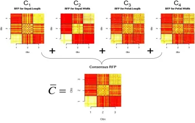
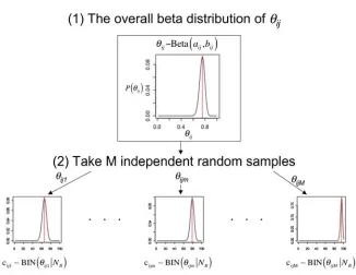
(7) However employing binary substitution on the categorical responses assumes a Euclidean relationship between categorical and continuous variables and homogenous levels within each categorical variable (Kaufman and Rousseeuw 1990).. It is. expected that for a realistic analysis this assumption may not be valid.. Motivated by the need to further understand which variables relate to the groups observed within the proximity matrix, the second mixed type extension proposed is to intelligently combine individual variable RF proximity matrices to produce a single overall consensus matrix. To do this the three combination methods are explored, General Procrustes Analysis (GPA), a Beta Binomial model (Gelman, Carlin, Stern and Rubin 1997) and Plaid Models (Lazzeroni and Owen 2002).. As this approach models a variable’s proximity matrix it is independent of its data type, therefore allowing it to produce a consensus matrix from proximities created from a mixed type data set. Furthermore as the individual variable proximity matrices are predicted by the overall consensus a R2 can be defined as a measure of variable importance is to the final cluster solution can be computed. A MCT is then used to identify the groups within the overall consensus based on decision rules found within the original dataset variables.. In Section 2 the background literature for clustering and profiling with a particular focus on ensemble and tree-based methods is reviewed. Section 3 describes the specifics of the core methods required to understand MCTs including univariate and multivariate tree models, tree-based ensembles, mixed type extensions to trees and methods to combine proximity matrices are described. Section 4 presents the MCT. 6.

(8) ?;. algorithms using the iris dataset as an example and Section 5 references the software used and developed in this thesis. Sections 6 and 7 use simulated and benchmark examples to assess and compare the performance of individual trees, tree-ensembles for profiling and MCT methods. Section 8 and 9 present a detailed discussion on the performance of the methods and conclusion chapters..

(9) 2. Background. 8.

(10) 2.1 Relating Objects Measures of how related objects are within a dataset forms one of the core principles of statistics.. How objects are related depends on their data types.. Two broad. statistical groups of variable types exist: quantitative and qualitative. Quantitative or ‘continuous’ variables comprise of two subgroups, interval and ratio. These variables have a strict order and are commonly used to measure the relative magnitude of an observation, e.g. temperature. Qualitative or ‘categorical’ variables also have two subgroups: ordinal and nominal.. However nominal qualitative variables can be. unordered and their assigned labels may not be representative of the actual levels within the variable. Categorical variables are often used to identify grouping structure over a variable e.g. hair colour.. Due to the structural difference between the. variables, separate measures for relating objects within a single data type have been developed.. For relating objects based on quantitative variables the most common choice is the Euclidean distance (Everitt 1993). The Euclidean distance between two vectors x ! and y is defined as, !. ( ) ( x! ! y! ) ( x! ! y! ) .. d x, y = ! !. T. (2.1). The interpretation of (2.1) is the length of a straight line between the two vectors and therefore assumes a continuous domain. As the length of the line increases the less related the two observations are and therefore the Euclidean distance is also a dissimilarity measure.. 9.

(11) Common choices for relating objects based on qualitative variables are a simple pairwise matching statistic (Kaufman, et al. 1990) that counts the number of observations over the variables with the same labels or using the chi-square distance (Lebart, Morneau and Warwick 1984). These are similarity measures as the more related the two objects are the larger the value of the measure.. 2.2 Relating Mixed Types Mixed type analysis relates variables spanning multiple data types. The problem surrounding this is the order inherent in quantitative variables and the lack of order of qualitative variables. This structural difference between the two types prevents any simple extension of a measure designed for a single type.. There are however,. approaches commonly used for relating mixed types. Two of these approaches are discussed in this thesis and are used as benchmark methods. These are using the Gower dissimilarity measure and binary substitution of categorical variables.. The first benchmark method for relating mixed types is the Gower dissimilarity measure (Gower 1971a). This is defined as, M. (. ). d xi , x j = ! !. "! m =1 M. (m ) (m ) ij ij. "! m =1. d. (2.2) (m ) ij. where dij(m ) is the distance between the observations i and j and carries a different definition given the type of variable m, and ! ij(m ) is a binary flag indicating the position of missing values within a variable. The definitions of dij(m ) are: 1. For nominal variables: 10.

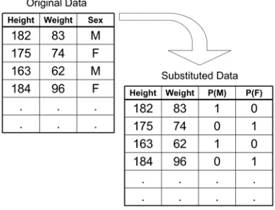
(12) dij(m ) = 1 if xim ! x jm. (2.3). = 0 if xim = x jm. 2. For binary variables, dij(m ) is the Jaccard Coefficient (Kaufman, et al. 1990). 3. For interval or ratio variables:. dij(m ) =. xim ! x jm. (2.4). range(xm ). This dissimilarity provides a simple measure between mixed types, however assigns the same weight to any variable type and therefore will not model complex relationships within the data.. Binary variable substitution for categorical variables is the second method for relating mixed types. This method substitutes categorical variables into an indicator matrix G (Young 1981, Gifi 1990). An example of binary substitution of a categorical variable (2.5) shows the indicator matrix G has a ‘1’ at the location of each category in the categorical variable xcategorical:. xcategorical. !1 #1 # #1 # #0 = [1,1,1, 2, 2, 2, 3, 3, 3] = # 0 # #0 #0 # #0 #0 ". 0 0 0 1 1 1 0 0 0. 0$ 0& & 0& & 0& 0& = G & 0& 1& & 1& 1 &%. (2.5). This substitution is made in optimal scaling, non-linear principal component analysis and correspondence analysis (Lebart, et al. 1984).. 11.

(13) Both the Gower dissimilarity and binary substitution assume Euclidean distances between categorical and continuous variables (Buuren and Heiser 1989).. This. assumption has considerable impact on the structure within the qualitative variables. It forces the assumption that the levels within these variables are homogeneous or evenly spaced (Kaufman, et al. 1990). Although, to identify a simple group structure this assumption may be valid, it is not likely to hold for more complex relationships. Therefore to find group structure over more complex relationships spanning multiple types a more advanced method for relating objects is required.. 2.3 Cluster Analysis The aim of cluster analysis is to find groups within a single dataset. There are many clustering methods available. Cluster analysis methods differ either in their definition of a group or in the algorithm used for finding the groups. Common group definitions of are either based on within group measures such as areas of high similarity between observations or between group measures such as the maximum distance between two objects (Figure 1).. Figure 1: Cluster analysis example.. 12.

(14) There are many algorithms commonly used for cluster analysis. Firstly, there are divisive or agglomerative methods, which iteratively separate or merge objects into groups. There are a variety of these methods such as hierarchical agglomeration (Everitt 1993) and auto-associative multivariate regression trees (AA-MRT) (Questier, Put, Coomans, Walczak and Vander Heyden 2004). Secondly there are optimisation methods that search for a predefined number of stable group centres. These methods define clusters by minimising the distance between objects and the group centres.. K-means and partitioning around medoids (PAM) (Kaufman and. Rousseeuw 1987) are examples of optimisation based methods.. 2.3.1 Hierarchical agglomeration. Hierarchical agglomeration iteratively merges the objects into groups starting with all objects in their own group or each object by itself. Using a specified agglomeration or merging criterion the algorithm searches for two objects to form the next best group. Once a group of more than one object is formed, these objects are considered. 13.

(15) a single group and treated as one for the duration of the algorithm. As the algorithm progresses all objects are placed into the group to which they are most similar, based on the agglomeration criterion. These groups are iteratively merged until the final group is the entire dataset. At any point in the agglomeration the algorithm may be stopped and the individual groups at that iteration can be extracted.. Different merging criteria will find different groups. Commonly used criteria are: 1. Single Linkage: The distance between two groups is the minimum distance between any two objects in separate groups. 2. Complete Linkage: The distance between two groups is the maximum distance between any two objects in separate groups. 3. Average Linkage: The distance between two groups is the average distance between all objects in both groups. 4. Wards Method: The distance between groups is defined by the change in within sums of squares between the merged and unmerged groups. Determining where to stop the merging determines the number of clusters that have been found. A plot of the agglomeration history called a ‘dendrogram’, for a small dataset can help to determine the stopping location. For large datasets however, these are difficult to read and no accepted automatic stopping criteria are available (Milligan and Cooper 1985).. 2.3.2 K-means and medoids (PAM). K-Means (Hartigan 1975) searches for the optimal set of clusters that minimise their within cluster sums of squares (WSS),. 14.

(16) K. WSS = #. # ( x!. k =1 xi "Ck. i. ! xk ) !. 2. (2.6). where xi is an observation vector in the dataset, Ck are the labels of the set of K ! clusters {1,!, k,!, K } and xk is the mean vector of cluster k. The user specifies the ! number of clusters to find and the algorithm starts with a randomly generated set of K cluster centres. Each object is then assigned to the centre it is closest to. After the assignment the cluster centres are re-computed and the objects re-assigned. The algorithm is stopped after the cluster centres have stabilised.. K-Means requires. quantitative variables as inputs. K-medoids is a robust form of K-Means as instead of minimising the within cluster sums of squares, it searches for representative objects within the dataset to form the cluster centres. These centres are selected such that the absolute distance between them is maximised. Partitioning Around Medoids (PAM) (Kaufman, et al. 1987) is an implementation of K-medoids. PAM is more robust than K-Means as the absolute distance between cluster centres is less affected by outlying observations than the squared distance.. 2.3.3 Clustering challenges. Cluster analysis is an unsupervised search for grouping structure within a dataset. However, as different groups are found using different techniques, verifying the accuracy of any clustering solution is difficult. The problem is a lack of a known objective to compare the final result against. This manifests itself in two major issues for any cluster analysis technique: 1. Estimating the number of groups to be found.. 15.

(17) 2. Verifying the accuracy, stability and reproducibility of these groups. These problems can never be fully resolved by any method. Despite this much research has been conducted with the aim to assist those implementing clustering analysis methods in validating their results.. 2.3.4 Determining the number of groups. The first studies into determining the number of groups in a dataset focus on automatic stopping rules for hierarchical agglomeration techniques. A stopping rule dictates where to stop merging objects to determine the number of groups found by the scheme. Comprehensive simulation tests of 30 of these criteria (Milligan, et al. 1985) revealed a clear best set of indices but also a wide variety of performances, and concludes unsurprisingly that the performance of each criterion is dataset dependent.. Predictive arguments for determining the number of clusters in a dataset are becoming more popular, as they can be explained in terms of model complexity. The elbow of the relative error curve of an Auto-associative Multivariate Regression Trees (AAMRTs) (Smyth, Coomans, Everingham and Hancock 2005) is an example of model complexity determining cluster number. Predictive cluster number determination treats cluster analysis as optimising the performance of a multivariate predictive model.. Mixture model based methods (Fraley and Raftery 2002) estimate the data using a weighted sum of distributions where each distribution corresponds to a group. Mixture models are predictive models of the data and as such use model complexity. 16.

(18) measures such as the Bayesian Information Criterion (BIC) and likelihood ratio statistics to determine the number of clusters. Although these measures are seen as a useful tool in practice, they assume a known structure on the data that is not nessarily valid (Mclachlan, Bean and Peel 2002).. The Gap statistic (Tibshirani, Walther and Hastie 2001) estimates the number of clusters by searching for the most reproducible set of labels. The Gap statistic, Gapn ( k ) = En* ( log (Wk )) ! log (Wk ). (2.7). observes the change in the log sum of the pairwise distances, log (Wk ) , for all objects in each cluster k on the real dataset, compared to the mean of the log sum of pairwise. (. ). distances for cluster k over many simulated reference datasets En* log (Wk ) . The gap statistic’s use of simulated reference datasets provides a null distribution upon which to compare a potential clustering solution against. The optimal number of clusters is found when the pairwise distances between objects in the actual scheme are most different to pairwise distances in the reference datasets. This is at the maximum of the gap statistic and the most reproducible number of groups.. Figure-of-merits (FOM) (Yeung, Haynor and Ruzzo 2001) are also based on the idea that model stability rather than pure predictive performance should determine the optimal number of groups. To determine stability, jack-knife cross-validation on the variables is employed. As the number of clusters is increased, the model stability is assessed by monitoring the change in the root mean squared error over the course of the jack-knifing. The result is a curve similar to the relative error curves produced by auto-associative multivariate regression trees (AA-MRT) however the focus is on stability not predictive performance. 17.

(19) The FOM approach is similar in ideology to that of Tibshirani et al. (2005) and (Dudoit and Fridlyand 2002) where V-fold cross-validation on the observations is used to assess cluster stability. Tibshirani et al. (2005) compares the performances of the same clustering model run on a test/training set partition of the data.. The. performance of the clustering algorithm is assessed by comparing the predicted groups using the training model on the test set, with the groups found by clustering the test set individually. If the groups differ then the clustering algorithm is not stable. Dudoit and Fridlyand (2002) perform a similar cross validation however build a classifier to predict the group labels of the training set. This classifier is then used to predict the test set labels. These methods test the reproducibility of a clustering scheme, where the most reproducible number of clusters is selected as optimal, they require no known group labels and unlike trees or mixture models are independent of the clustering method.. Once the number of clusters has been determined there is still the problem of assessing the accuracy of the solution. Even with the number of clusters estimated there are still a huge number of possible group configurations. The rand and modified rand indices (Hubert and Arabie 1985) are measures of overlap between two clustering schemes on the same data set. If two different clustering schemes on the one dataset find similar grouping structure, then it is likely that the found groups are representative of the dataset. This is a relative form of accuracy, however as the group labels are unknown it is the only form of accuracy possible.. 18.

(20) One solution to the problem of determining which clustering algorithm to use is by combining information over many different clustering algorithms. Such an approach is called an ensemble approach to clustering and is now discussed in more detail.. 2.3.5 Cluster ensembles. A cluster ensemble (Strehl, et al. 2002) is simply a collection of clustering solutions that are combined into one overall solution. An individual clustering solution is called a partition within the cluster ensemble. The goal of the analysis is to find common grouping structure across each partition and summarise it into one overall partition. This is done to remove the need to choose which clustering method to use. Instead, a range of techniques are selected and the ensemble combines them into an overall partition which is the final grouping structure of the data. It is hoped by combining information across many solutions that the stability of the final clustering structure is improved.. 2.3.5.1 Cluster ensemble objective functions. To find the overall partition requires a means of summarising common information across many different partitions. Functions that do this are called ensemble objective functions. In fact there are many potential statistics that can be employed as an objective function for cluster ensembles. The goal of a cluster ensemble is to find an overall partition that optimises this objective function.. 19.

(21) Cluster ensembles were initially defined using the maximum of the normalised mutual information index, ! NMI , between two partitions (Strehl, et al. 2002, Ana L. N. Fred and Anil K. Jain 2005) as its objective function:. !. ( NMI ). (". (a). ,". (b). ). # nl(h)n & 2 k k (h) = ) ) nl log k ( a ) .k ( b ) % (h) ( n l =1 h =1 $ n nl ' (a). (b ). (2.8). In (2.8) the two partitions ! (a) and ! (b) on n observations have k (a) and k (b) groups where n (h) is the number of observations is cluster h according to ! (a) , nl is the number of observations in cluster l according to ! (b) and nl(h) is the number of observations in cluster l according to ! (b) that are also in cluster h according to ! (a) .. Defining (2.8) as the ensemble objective function, to find the overall partition !ˆ , will require a search over permutations of all labels within each partition in the set of all. {. }. partitions, ! = " (1) ,!, " (q) ,!, " (r ) . kn. Unfortunately this requires approximately. k! comparisons between groups where n >> k which is infeasible if the number of. partitions is large (Strehl 2002). To bypass this computational complexity, cluster ensembles use heuristics to approximate !ˆ .. Another objective function commonly used defines the Euclidean dissimilarity (Weingessel, Dimitriadou and Hornik 2001) between two partitions to be,. (. ). d ! (a) , ! (b) = min " ! (a) # ! (b)". where the minimum is taken over all possible permutations ! , and. (2.9) .. is the. Frobenius norm. The minimum of (2.9) is found when the permutation performed on. ! (b) matches best the group configuration in ! (a) .. 20.

(22) A solution to (2.9) is possible by treating the problem as a linear sum assignment problem and using a linear program to estimate the overall partition (Hornik 2006). By extending (2.9) to the squared Euclidean dissimilarity,. (. ). {(. d ! (a) , ! (b) = min ! (a) " ! (b)#. )} 2. (2.10). another possible solution can be found using the iterative approach described in the “Voting” algorithm (Weingessel, et al. 2001). This algorithm iteratively updates the probability that each observation lies within each group over all partitions within the ensemble.. The group with the maximum probability is the final clustering. assignment.. Hypergraph representations of the ensemble as in Hypergraph Partitioning Algorithm HGPA, Meta-Clustering Algorithm MCLA (Strehl 2002) and Hybrid Bipartite Graph Formulation HBGF (Fern and Brodley 2004) also present a possible means for estimating the overall partition. These methods represent each cluster in the ensemble as a vertex on a graph that are connected by common observations.. From this. representation, a distance between clusters can be formulated, and the goal of the analysis is to collapse the graph into strongly connected components that define the overall partition.. Mixture model approaches can also be used to estimate the overall partition (Topchy, Jain and Punch 2004, Topchy, Minaei-Bidgoli, Jain and Punch 2004). Here each partition within the ensemble is treated as a random variable that can be modelled with a mixture of multivariate component densities,. 21.

(23) (. ). r. (. P !q " = % # q P !q $ q q =1. ). (2.11). where !q is a partition in the ensemble with component density parameters ! q and. ! q are the mixture weights and ! is the set of all parameters of the mixture model to be estimated ! = {"1 ,…, " r ;#1 ,…,# r } . The final cluster assignments are found by estimating the maximum posterior probability of each observation belonging to each component density in the mixture model.. 2.3.5.2 Cluster ensemble consensus matrices. The most common solution to cluster ensembles avoids optimising an objective function entirely through the construction of a ‘consensus’ or ‘co-occurrence’ matrix over the observations. A consensus matrix is a similarity matrix where each cell contains a count as to how many times two observations are clustered together over all partitions in the ensemble. Once constructed from an ensemble this matrix is passed as an input to another clustering algorithm to find the overall partition. Examples of this approach can be found in the Cluster-based Similarity Partitioning Algorithm (CSPA) (Strehl, et al. 2002) and the evidence accumulation algorithms (Ana L. N. Fred, et al. 2005). CSPA clusters co-occurrence matrices using the hypergraph partitioning algorithm METIS (Karypis and Kumar 1998) and evidence accumulation using hierarchical agglomeration with single linkage (Section 2.3.1).. One approach to constructing a consensus matrix is by bootstrapping a clustering algorithm and computing the similarity based on the partitions from each bootstrapped model (Monti, et al. 2003). Bootstrapping for consensus construction. 22.

(24) has been applied to hierarchical agglomeration (Kavsek, Lavrac and Ferligoj 2001, Monti, et al. 2003, Stephen Swift, et al. 2004), PAM (Dudoit and Fridyland 2003) and self organising maps (SOM) (Monti, et al. 2003), and has consistently shown to improve the stability of the groups found. Furthermore, observation of the consensus matrix reordered by the found clusters provides a useful visualisation tool to assess the quality of the groups found (Ben-Hur, Elisseeff and Guyon 2002, Monti, et al. 2003).. Analysis of the structure within consensus matrices provides a method to estimate the optimal number of groups (Ben-Hur, et al. 2002, Monti, et al. 2003). This work assumes that an ideal consensus matrix is block diagonal and sparse. Therefore an ideal distribution for a consensus matrix can be estimated. This distribution can be viewed by a histogram, and should show two clear bins, one for the observations classified together and one for the observations not classified together. By computing the empirical cumulative distribution function (CDF) of the histogram and observing its structure a measure of quality for that scheme is produced. By observing changes in the CDFs of the same method grown to different numbers of clusters an estimate of the optimal number of clusters can be achieved. Cluster ensembles show that by optimising the level of agreement between different clustering regimes, uncertainty in choosing the clustering method and estimating number of groups can be reduced. However these methods do not take into account to the accuracy of the clustering method. In fact a danger of these methods is that in combining many partitions without knowledge of how representative each solution is of the data it is possible to find a stable set of clusters with no accuracy. One solution to this problem is to consider each clustering algorithm as a prediction of the dataset.. 23.

(25) By doing this ideas from predictive ensembles can be used to assess the accuracy of a cluster ensemble.. 2.3.6 Cluster ensembles and predictive ensembles. By bootstrapping a clustering technique and aggregating the results, consensus clustering is essentially ‘bagging’ a clustering algorithm (Breiman 1996a). Usually bagging is a methodology that aims to optimise performance of a model by averaging over many bootstrapped predictions. In random forests it is shown that bagging treebased models can dramatically improve their predictive performance (Breiman 2001). Furthermore, a random forest provides a means of summarising the structure found over all trees generated over the course of the bootstrapping through the construction of a proximity matrix. The random forest proximity matrix is similar to a consensus matrix, as it is a similarity matrix comprising of a count of how many times two observations have been placed in the same terminal node over an ensemble of trees within the forest.. An unsupervised extension to random forests, (unsupervised. random forests), has allowed for this matrix to be constructed on a single dataset by using a simulated response variable. Unsupervised random forests (Shi, et al. 2006) is a ensemble clustering algorithm that produces a consensus matrix and employs PAM on the proximity matrix to find the overall partition.. This method exploits the. advantages of consensus clustering, however as it uses a meaningless simulated response it nullifies the predictive improvements offered by random forests.. This thesis presents a new approach for cluster analysis of a mixed dataset called Multivariate Consensus Trees (MCT).. MCTs exploit the similarity between the. 24.

(26) predictive proximity matrix of tree-based ensembles and the cluster ensemble consensus matrices. Combining the two ideas allow MCTs to harness the predictive power of tree-based ensembles, and by using cluster ensembles, to present this information in the form of a consensus clustering problem. Furthermore as trees are a model based clustering approach, MCTs also provide measures to estimate the optimal number of clusters and to assess the accuracy of the final solution.. MCTs predict each variable within the response set with a tree-based ensemble. From these ensembles the grouping structure from each variable is summarised into a proximity matrix. Then in a similar step to ensemble clustering these proximity matrices are combined into one overall consensus matrix. This consensus matrix provides an overall view of the group structure within the entire dataset. By searching for a decision within the original variables of the dataset, a tree is grown to partition this overall consensus matrix. The resulting tree is the called the MCT of the dataset and the groups found lie in the terminal nodes.. By predicting each variable individually MCTs perform a similar step to the cross validation used in FOMs, and allow for a way to assess how representative each variable is of the final clustering solution. This addresses the previously mentioned problem associated with consensus ensembles in assessing the accuracy of the final solution. Furthermore, knwledge of individual performances for each variable allows MCTs to perform a data reduction step to remove unimportant variables from the analysis.. Variable selection performed in MCTs can reduce a highly complex. clustering problem into a simpler one allowing for easier understanding of the final solution.. 25.

(27) MCTs as a cluster analysis method use auto-association as in AA-MRT on the dataset to produce the tree. However as trees can predict a separate response dataset, MCTs can also be used as a multivariate profiling tool. In the next section common profiling methodology is discussed.. 2.4 Profiling Analysis The process of identifying groups in one dataset (the predictor set) that also define groups in another (the response set), is in this thesis is “profiling the response dataset by the predictor set dataset”. The response Y = !" y1 , y2 ,…, ym ,…, yM #$ consists of n ! ! ! ! observations on M variables where each response variable is denoted by ym , and the ! predictor set X = !" x1 , x2 ,…, x p ,…, xP #$ on the same objects as the response set but on ! ! ! ! P separate predictor variables denoted as x p . The response set is usually a small ! quite specific set of variables relating to the phenomena under consideration. However, it is common for the predictor set to consist of a comparatively large number variables that may be related to the response.. In this case the researcher. wishes to identify a small subset of predictor variables that summarise strong relationships.. Simply clustering the profiling set is an insufficient solution to profiling analysis, as the same grouping structure may not be present in the predictor set (Figure 2). Profiling methods require a compromise solution between the groups present within both the response and predictor datasets. If a group exists within the response set that. 26.

(28) is not represented within the predictor set then it will not be identified by a profiling method. Therefore profiling is a data mining problem as it involves identifying the important structure within the predictor variables that agrees with the structure of the response set. This requires a method that can not only relate objects within an individual dataset but also between datasets.. 27.

(29) Figure 2: Example of profiling a response set Y = {y1, y2} by predictor variables X = {x1, x2, x3, x4}.. Relating two complete datasets is a difficult statistical problem and requires the specification of a statistical model. Multivariate Analysis Of. Methods like multivariate regression and. Variance (MANOVA). (Seber. 1984),. Canonical. Correspondence Analysis (CCA) (Hotelling 1936), Generalised Procrustes Analysis (GPA) (Gower 1975) all relate information from many sources. These methods however are either aimed more at explicit prediction or summarising the relationships in a lower dimension rather than profiling any group structure that may be present across the datasets. Rule based methods are also commonly used as profiling tools aimed at identifying groups over many databases. However, for reasonably sized datasets, these methods require summarising thousands of individual rules.. 28.

(30) 2.4.1 Multivariate regression and multivariate analysis of variance. Multivariate experimental design is the most common example of profiling in statistics.. The model for both multivariate regression and analysis of variance. (MANOVA) is stated in the form of a general linear model,. Y. (N ! M ). = X. B + U. ( N ! P) (P ! M ). (2.12). (N ! M ). where B is a matrix of coefficients estimated by least squares and U is the corresponding error matrix. If X is a matrix of predictor variables then the model in (2.12) is identical to performing separate univariate multiple regressions for each response variable. However if X is substituted for an ANOVA design matrix, solving (2.12) is performing a multivariate hypothesis test. The major assumption of these models is that the error matrix U follows a multivariate normal distribution. Multivariate linear models of this type are designed to predict Y. They do not uncover common groupings unless they are known and coded into the design matrix.. 2.4.2 Canonical correlation analysis (CCA). Canonical Correlation Analysis (CCA) models common correlation structure between Y and X by summarising them in a lower dimensional space. These dimensions, ui ! and vi are weighted projections of Y and X: ! ui = ai T Y , ! ! vi = bi T X ! !. (2.13). where ai and bi are called the canonical variates. The canonical variates are found in ! ! directions of decreasing maximum squared correlation r 2 between ui and vi . The ! ! canonical variates are a mapping between Y and X.. The maximum number of 29.

(31) canonical variates that can be extracted is less than or equal to the smallest number of variables present in either Y or X (Seber 1984). These variates have mathematical relationships with the results of multivariate regression and MANOVA, but also with linear discriminate analysis and so may highlight group structure between the two datasets (Rencher 2002).. 2.4.3 Procrustes analysis. Methods such as CCA require the specification of a response and predictor set, and as such only work for relating two datasets. Methods of combination like Generalized Procrustes Analysis and Individual Scaling Analysis (INDSCAL) (Carroll and Chang 1970) relate many datasets together in order to find a matching configuration. Over M datasets these methods minimise, 2' $M min % # ! m X m " X ( & m =1 ! ). (2.14). where the matching configuration is X and ! m is a weight vector that defines a rotation upon X m such that it is closest to the mean configuration. This mean configuration highlights dominant structure over all data sources. However as the purpose of these methods is as a data reduction tool, it is difficult to identify the source of the observed groups.. 30.

(32) 2.4.4 Decision and association rules. Association rules are logical expressions found within a dataset that are characteristic of, or are related to an outcome.. Used commonly in “market basket analysis”. (Giudici 2003) the association rules are of the form,. d(x) ! y. (2.15). where d(x) is a decision rule on a variable x that logically implies y. The form of d(x) can be in the that of a single variable inequality or as a logical combination of inequalities using “and” (∧) and “or” (∨) operations (Lent, Swami and Widom 1997). As this definition is quite flexible association rules can be easily defined for all data types.. For any realistic analysis thousands of individual association rules are identified. This means a way of filtering to find only interesting or significant association rules is needed. This brings forward the ideas of support and confidence for an association rule. For the simple rule d ( x ) ! y the support S and confidence C are defined as,. S = P ( A ! B). C = P ( B A). ,. (2.16). where the support is the probability of both events A and B occurring together, and the confidence is the probability of event B given an event A. Identifying interesting rules is usually done by imposing a threshold on either the support or confidence on individual rules (Srikant and Agrawal 1997), or by constructing a weighted combination of rules based on how well they predict a response (Friedman and Popescu 2005).. 31.

(33) A Classification and Regression Tree (CART) is a hierarchical combination of decision rules and is often referred to as a decision tree (Kass 1980, Breiman, et al. 1984). Extensions to CART for multivariate regression (MRT) (Yan Yu and Diane Lambert 1999, De'ath 2002, Larsen and Speckman 2004) allow for profiling a continuous response set, by a mixed predictor set. Auto-associative Multivariate Regression Trees (AAMRT) (Questier, et al. 2004) look for decision rules that partition a continuous profiling set into homogeneous clusters, allowing for MRTs to work both as a profiling and clustering tool. Furthermore these decision rules can then be used to cluster new observations. This also allows for validation regimes to be imposed over the model to test for validity and help estimate the number of groups present (Smyth, et al. 2005).. The flexibility of decision rule methods to handle most data types is their most powerful feature. When combined into a decision tree they provide an intuitive statistical framework to conduct profiling analysis. Furthermore ensembles of trees not only improve and stabilise the predictions of a single tree but also provide useful links with cluster ensemble methods (Section 2.4). Therefore tree-based methods are a natural choice for profiling analysis and are the focus of this thesis.. 2.5 Tree-based Profiling Tree based techniques present an ideal framework for profiling as they produce predictive decision rules on the predictor variables that identify group structure within the response. The primary aim of this thesis is to extend tree based profiling to. 32.

(34) handle a mixed type response set. To achieve this goal several approaches are implemented in this thesis culminating in the development of MCTs.. Mixed type extensions to standard CART theory are proposed using the Gower dissimilarity and binary substitution. These methods transform the response dataset into a form suitable for use with the existing MRT or Db-MRT methods. Furthermore through the use of auto-association these techniques double as a clustering tool. The result of this is a single multivariate tree that can profile a simple mixed type response set.. Binary substitution represents a mixed type dataset set as a multivariate continuous dataset compatible with MRTs and therefore allows a simple mixed type extension to multivariate ensemble methods. In this thesis MRT theory with binary substitution is used to implement multivariate mixed type extensions to random forests and treeboost. Multivariate random forests and treeboost are predictive clustering or profiling techniques that can handle multivariate response and predictor sets and are resistant to a large number of variables within the predictor set.. Through the use of the proximity matrix arising from tree-based ensembles this thesis proposes MCTs, which is a new technique for either profiling or clustering. MCTs present methods to intelligently combine individual ensemble proximity matrices to allow for improved understanding of the structure within each response variable.. By partitioning these combined ensemble proximity matrices. MCTs provide a method to identify grouping profiles found over all ensembles. This. 33.

(35) allows for removal of unimportant response variables from the analysis and more importantly allow MCTs to identify subgroups of variables within the response set.. 34.

(36) 3. Methods. 35.

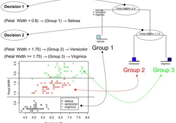
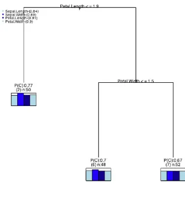
(37) In this section is the core theory that forms the base of the MCT model. Firstly the CART methodology is described along with the relevant multivariate extensions MRT, AA-MRT and Db-MRT. This is followed by multivariate extensions to treebased ensembles. From here, the link between tree-based ensembles and cluster ensembles is made by describing techniques to combine ensemble proximity matrices.. To assist the reader in interpretation of the models presented here an example implementation is provided on the benchmark iris dataset (Fisher 1936).. 3.1 Tree-based Models A decision tree is a hierarchy of decision rules that partition a response into separate groups (Figure 3). This hierarchy imposes interactions between decision rules using an “and” operation. Figure 3 presents an example decision tree to classify three varieties of iris flowers (Setosa, Versicolor and Virginica) based on their sepal and petal length and widths using the benchmark iris dataset. The first decision or split is found on the variable “petal width”. The effect of this split is to partition the dataset into two mutually exclusive groups; the first containing iris flowers with a petal width less than 0.8 and the second with petal widths greater than 0.8. This decision has the effect of accurately defining the Setosa variety of iris flower in the left terminal node (3.1). From the scatter plot in Figure 3 it is obvious that based on petal width the Setosa variety of flowers is the most easily identified showing a considerable smaller petal width and is therefore the first split within the tree.. 36.

(38) (1) {(Petal Width < 0.8) ! (Group 1) ! Setosa}. (2) {(Petal Width >= 0.8) " (Petal Width < 1.75) ! (Group 2) ! Versicolor} . (3.1) (3) {(Petal Width >= 0.8) " (Petal Width >= 1.75) ! (Group 3) ! Virginica}. From here the tree must further partition the dataset to identify the other two varieties of iris flowers. As the first split accurately determined Setosa in the left terminal node, the second split to determine Versicolor and Virginica must be on the right. By coincidence this split is also performed on petal width, however could have potentially been on any other predictor variable within the dataset. As the second split depends on the first, to determine the two other varieties of iris flowers the compound decision rules in (3.1) are necessary. By observation of the scatter plot in Figure 3 it can be seen that this decision is not as clear as the first. In fact, this split invokes a misclassification of 6 out of the 150 iris flowers.. Figure 3: Example decision tree classifying the species of flowers in the iris dataset.. 37.

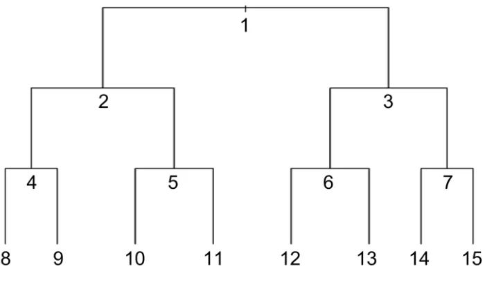
(39) In this example the tree built is a classification tree and the splits are performed on quantitative variables. However, the flexibility of tree based models comes from the easy definition of decision rules for either categorical or quantitative predictor variables, for either univariate classification or multivariate regression. There are two popular tree growing algorithms available, Classification and Regression Trees (CART) (Breiman, et al. 1984) and C4.5 (Quinlan 1993).. Due to the easy. accessibility of the “rpart” package (Therneau, Atkinson and Ripley 2005) in R (R Development Team 2005) to benchmark the CART algorithm, this framework is selected for use in this thesis.. 3.2 Classification and Regression Trees (CART) Building a CART model requires a search on two levels (Figure 4). Starting with all observations within the root terminal node, the first step is to find the next best split for each terminal node of the tree. This involves searching in every terminal node for the decision rule that minimises the impurity defined in (3.2). After all the next best splits have been found for each terminal node, a second search is performed over the terminal nodes of the tree. By minimising relative error (RE) of the tree defined in (3.3) the best node to split on is found. This split is then used to grow the tree. This process continues until no more splits can be found; this tree is called the maximal tree.. 38.

(40) Figure 4: CART algorithm. While tree size < maximum tree size do: 1. Find the best split on each terminal node: a. For each predictor variable find the best split, d, by finding the minimum impurity R(d) (3.2). b. Over each predictor compare the best splits, and pick the variable with the smallest R(d). This split on this variable is the next best split for that terminal node. 2. For each terminal node compute the RE(d) (3.3) using the next best split for that terminal node. 3. Compare the RE(d) statistics over each terminal node and grow the tree on the minimum.. CART finds the next best split for each terminal node by ranking all possible decision rules within the predictor set. Each decision rule is assessed based on its impurity. The impurity of a decision is defined as the degree of heterogeneity of the response observations within each node resulting from the decision. Put more formally, the impurity R(d) of a decision d is defined as the weighted sum of the impurities of the. (. ). (. ). left, R y !left and right R y !right nodes respectively, ! !. (. ). (. R ( d ) = pleft R y !left + pright R y !right ! !. ). (3.2). where pleft and pright are the probabilities of the left and right nodes respectively.. CART defines the idea of a relative error (RE) to assess the quality of the overall tree. The RE(T) of a tree T, is defined as the sum over the impurity of all terminal nodes,. RE(T ) =. " R ( y !t. t n !T. ! R y !. (). n. ). (3.3). (). where tn is a terminal node is tree T and R y is the relative error of the non! partitioned response. As defined in (3.3) the RE is the percent error of a tree, and is a monotonically decreasing function.. 39.

(41) 3.2.1 Determining CART tree size. The algorithm in Figure 4 grows the maximal tree, and will result in a tree that overfits the data. Therefore a means of pruning the tree to a smaller size is needed. Tree size can be defined in two ways; either by specifying the minimum size of the terminal nodes or by specifying the maximum number of splits. The values of these parameters are most commonly estimated using V-fold cross validation.. This. involves the CART algorithm (Figure 4) to be run V times on subsets of the data. For each subset and for each tree size (1 split, 2 splits, … , etc.) the data not used to build the tree is predicted or classified.. After the V iterations, the cross validated. performances are presented on a graph called the relative error graph (Figure 5). The minimum of the cross validated RE graph is taken to be the optimal tree size for that dataset.. An example of a RE curve for a multivariate regression tree on the iris dataset is presented in Figure 5. This graph contains two plots corresponding the training set (top) and test (bottom) relative errors for tree sizes ranging from 1 to 10 splits. The reference line displays the mean performance for each tree size. For standard CART models 10-fold cross validation is usually implemented. The points surrounding the line are the individual performances for each tree over the course of 10-fold crossvalidation. The spread of the points around the mean line at each tree size is related to how certain a tree of that size is. If the variance of the points is large then the structure of a tree grown to that size is uncertain. The task is now to estimate an appropriate tree size based on these graphs.. 40.

(42) Figure 5: 10-fold cross-validated RE graph for the iris dataset.. Picking the optimal tree size can be done in many ways. The most common method is the “1-SE” rule. This rule defines the best tree to be the simplest tree with a RE within one standard error of the RE of the next tree. This implies that the RE of the next tree is essentially the same as the RE of the current tree, and then there is no improvement gained by growing the tree any further. The idea of the “1-SE” rule method is that the terminal nodes of the tree must be as stable as possible. As this thesis is focused finding stable groups within the terminal nodes of a tree, this method is employed to determine optimal tree size.. Minimal cost-complexity is another means to determine the size of CART models that is focused on optimal predictive performance (Breiman, et al. 1984).. This rule. estimates a penalising parameter that is a combination of the predictive performance of the tree and its complexity. The form of this penalty is, 41.

(43) RE! (T ) = RE (T ) + ! T!. (3.4). where RE! (T ) is a combination of its cost RE(T) and its complexity ! T! with T! being the number of terminal nodes in a tree and ! is the estimated cost complexity parameter.. The best tree is now picked at the minimum of (3.4) which is the. minimum error tree given its size. Many other pruning algorithms exist for finding the optimal tree, such as Reduced Error Pruning (REP) and Pessimistic Error Pruning (PEP) (Quinlan 1987). For a comparison of the relative performances of these see (Esposito, Malerba and Semeraro 1997, Esposito, Malerba, Semeraro and Tamma 1999). 3.2.2 Finding the best split. Making a decision upon a variable requires an exhaustive search over all possible split points within each predictor variable. For continuous predictor variables sorting the response such that it is in the ascending order of the predictor variable, and then parsing it in this order will search all valid splits.. In general for a continuous. predictor variable there are n valid split points. For a categorical predictor variable with k levels a search over all (2k-1-1) possible splits is required. At each split point the impurity function, (3.2), must be evaluated and compared with the current best split. The specific impurity function used depends on the types of variables within the response set. Common impurity functions for classification and regression are now discussed.. 42.

(44) 3.2.3 Classification trees. The gini index for a split, d, is the sum of the gini indices for the left and right nodes resulting from the split,. ! ! nLeft $ # R (d ) = # ) p ( yi = k )(1 ' p ( yi = k )) " n &% # k (levelsy " yi (Left. (. ! ! nRight $ # +# ) p ( yi = k )(1 ' p ( yi = k )) " n &% # k (levelsy " yi (Right. (. $ & & %. $ & & %. ). ,. (3.5). ). where p ( yi = k ) is the probability that an observation yi is of class k within the left or right nodes, levelsy is a list of all the groups within y, nLeft and nRight are the number of observations in the left or right nodes respectively and n is the total number of observations . It is possible to simplify (3.5) further and get a more interpretable from of the gini index: ! $ ! $ ! nleft $ # ! nRight $ # 2& 2& R (d ) = # 1 ' ) p ( yi = k ) + # 1 ' ) p ( yi = k ) . & " n &% # k (levels & " n &% # k (levelsy " yi (Left % " yi (Righty %. (3.6). As indicated in (3.6), minimising the gini index requires either p(yi=k) to be close to 1. In other words minimising the gini index will find terminal node class profiles with probabilities of each class being close to 1. Taken to its extreme this usually results in terminal nodes containing yi’s of the same class. After the tree is grown, classification trees use the highest probability class within a terminal node to classify the observations within that node.. 43.

(45) 3.2.4 Univariate regression trees. Regression trees minimise the squared error between all observations and their mean within a terminal node, ! nLeft $ R(d) = # ) yi ' yLeft " n &% yi (Left. (. ). 2. ! nRight $ +# ) yi ' yRight " n &% yi (Right. (. ). 2. (3.7). where yLeft and yRight are the means of the observations in the left and right partitions respectively. In implementing (3.7), the squared error must be computed for all possible splits in each predictor variable. This is time consuming and not necessary as (Therneau, et al. 2005) show that maximising the within sums of squares over the entire split (both left and right terminal nodes) produces the same split and is considerably faster , *! nLeft $ 2 2! nRight $ min ,# yi ' yLeft + # yi ' yRight / 0 ) ) & & " n % yi (Right +" n % yi (Left . , *! nLeft $ 2 2! nRight $ max ,# +# yRight / i ' yt i ' yt & yLeft " n &% +" n % .. (. (. ). ). (. (. ). ). (3.8). where yleft and yright is the mean of the left and right terminal nodes of the split respectively and yt is the mean of all observations in the parent node.. From (3.8) it can be seen that a split in regression trees can be viewed as either finding the maximum difference between the terminal node means and the total means; or, by (3.7), the same split is found by minimising the variance within each terminal node. The overall prediction made by a regression tree is the mean of each terminal node.. 44.

(46) 3.2.5 Multivariate regression trees (MRT). Multivariate regression splitting (MRT) is simply the multivariate extension to (3.7) (Segal 1992, Yan Yu, et al. 1999, De'ath 2002, Larsen, et al. 2004), M ! nLeft $ R(d) = # ( ( yim ' yLeft , m " n &% yi )Left m =1. (. ). 2. M ! nRight $ +# ( ( yim ' yRight , m " n &% yi )Right m =1. (. ). 2. ,. (3.9). where yLeft , m and yRight , m are the means of the mth response variable in the left or right nodes respectively. Minimising (3.9) is analogous to maximising the Mahalanobis distance with a covariance matrix equal to the identity (Segal 1992). Furthermore if the response matrix Y is a binary indicator matrix for a categorical variable as in (2.5), it can be shown that minimising (3.9) is the same as minimising the gini index (3.6) (Breiman, et al. 1984). This improves our understanding of the gini index: in that for classification splitting it directs the algorithm towards finding the split that minimises the variance of the probabilities for each level within a node (Hastie, Tibshirani and Friedman 2001).. MRTs offer a method for a continuous profiling set and a mixed predictor set because the tree is identifying groups (terminal nodes) within a response matrix Y that are defined by the predictor set X. MRTs identify stable and reproducible clusters, as the terminal nodes must be predictive of the response. Furthermore, the elbow of the relative error curve (Figure 5) which is used to estimate tree size also gives an estimate of the number of groups in the profiling solution (Smyth, et al. 2005). This is a validation regime over the profiling technique because the RE curve provides a cross validated procedure for estimating the number of groups based on predictive performance. This links in with the concepts of cross-validation (Dudoit, et al. 2003). 45.

(47) and predictive validation (Dudoit, et al. 2002, Tibshirani, et al. 2005) for cluster validation.. 3.2.6 CART on a distance matrix (Db-MRT). A distance matrix is a specific data type that summarises relationships between observations within a dataset. It is a square symmetric matrix of the form,. ! # #d D (Y ) = # # # #d ". 0. ( y! , y! ) 2. 1. (. d y1 , y2 ! ! 0. ). #. ( y! , y! ) N. 1. ". (. ). " d y1 , yN $ ! ! & & & & $ & & 0 %. (3.10). where D(Y) is a distance matrix of size n by n, where n is the number of observations,. (. ). d yi , y j the distance between observations i and j in the response dataset Y. Forming ! !. splits on the distance matrix representation of the response set has been suggested as a flexible multivariate extension to CART (De'ath 2002).. As a distance matrix contains the observations on both the rows and columns, a split must also act on both. Figure 6 shows a distance matrix D(Y) is partitioned by a decision d(x) on predictor variable x. This results in four sub-matrices corresponding to the left group (DL), right group (DR) and the between group distance matrices which for ease of understanding in this thesis are called the covariance groups, (DC) and (DC)T.. The goal of a partition is to minimise the distances between the. observations within both the left and right groups.. 46.

(48) Figure 6: Example distance matrix partition.. Distance Based MRT (Db-MRT) (De'ath 2002) defines the node impurity as the sums of the squared distances within the left and right groups,. R (d ) =. 1 # " nL2 %$ i!DL. &. 1 #. &. " d ( y , y ) (' + n %$ " " d ( y , y ) (' 2. j !DL. i. ! !. j. 2 R. 2. i!DR j !DR. i. ! !. j. (3.11). which is exactly equivalent to standard MRT (3.9) if the distance metric between two observations is squared Euclidean, however takes no account of the distance between the observations of the two groups found in DC .. If the distance in (3.11) is. Euclidean, the squared distance between the left and right group centroids can be defined by the Gower distance (Gower and Hand 1996), d ( DL , DR ) = DL + DR ! 2DC. (3.12). where DL , DR and DC are the centroids for each sub-matrix and are defined to be,. Dg =. (. ). 1 " " d yi , y j , ng2 i!g j !g ! !. (3.13). where g denotes either the left, right or covariance sub-matrices. Either maximising (3.12) or minimising (3.11) is simply stating that the distances between objects within a cluster must be small. However it does not necessary follow that minimising (3.11) will maximise (3.12), due to the inclusion of the covariance group centroid in (3.12). 47.

(49) Tree based-distance splitting has the ability to profile group structure within a multivariate response. Furthermore it allows for profiling over a mixed type through the use of the Gower dissimilarity to construct the base matrix to be partitioned. However as a distance matrix is an abstraction upon the data, assessing predictive performance is difficult. This difficulty extends to problems in determining which response variables are expressed within a terminal node.. 3.2.7 Auto associative multivariate regression trees (AA-MRT). Trees can be considered a search for homogeneity within the response. Multivariate regression and Euclidean Db-MRT have strong relationships with K-Means and Wards method for agglomeration, as they all define a group by minimum withingroup sums of squares. However unlike the other techniques MRTs use a predictor set to identify the groups.. Auto-Associative MRTs (AA-MRT) (Questier, et al. 2004, Smyth, et al. 2005) extend MRTs to be able to cluster a single dataset. The idea simply mirrors the response set within the predictor set of the MRT model. For example, to cluster a dataset Y, AAMRT will grow a tree with Y as the response and predictor dataset. AA-MRT is a form of constrained K-means as the groups are found to reduce the within-sums-ofsquares but also must be defined by the decision rules of the tree.. 48.

(50) 3.3 Ensembles of Trees When modelling large datasets it is necessary to pick a model that can accurately assess the predictive performance of all predictor variables. Usually this is done as a two step procedure by first using a data reduction method, such as a partial least squares (De Jong 1993) or a genetic algorithm (Mitchell 1998). The output is then passed into a more powerful method for example see Hancock et al. (2005). Another alternative is to use a penalising method such as ridge regression (Hoerl and Kennard 1970) or penalised discriminate analysis (Hastie, Buja and Tibshirani 1995). Penalising methods impose strong conditions on estimation to reduce the risk of overfitting. However it is rapidly becoming clear that a single model is insufficient for analysing large datasets. More commonly, collections of models are combined into an ensemble to create an overall large model. By doing this, statisticians are treating a single model more as a variable within a larger modelling scheme.. A weak learner (Schapire 1990) is a model that is guaranteed to perform better than a coin flip.. CART falls into this category because the RE must be a decreasing. function. Therefore the worst possible performance of CART must still outperform the mean variation on the training set. As encouraging as this is, it is well known that the predictive or classification performance of CART is average to poor (Hastie, et al. 2001). However, weak learners like CART are ideal for ensemble methods, as it is known that any individual model produced must do better than random chance.. Ensemble methods combine the results of many weak learners to improve their overall predictive performance (Breiman 2001). Commonly behind these techniques. 49.

(51) is the idea of bootstrapping to improve the predictive performance of the model (Efron 1979). By taking random samples of the training set many different models can be built, each selecting different variables and displaying different characteristics. These models are then combined together using a simple linear combination. There are many different types of ensembles; the differences between them lie in how the linear combination of models is constructed.. Two common means of building. ensembles are bagging and boosting.. 3.3.1 Bagging, random forests and multivariate random forests. Bagging (Bootstrapped Aggregation) (Breiman 1996a), is the simplest means of building an ensemble. Bagging averages the results over many bootstrapped models. For discriminate analysis, the classification of a single observation is the majority vote over all bootstrapped models and for regression it is simply the mean prediction. Bagging usually performs better than a single model (Breiman 1996a), and also improves the accuracy of the variable importance statistics (Breiman 1996a, Dietterich 2000b).. A common extension of bagging is implemented using a CART model and in this form, it is called Random Forests (RF) (Breiman 2001). The difference is that the random forest bootstrap is performed over the variables and the observations simultaneously (Figure 7). This ensures that each tree has the best chance of being different. The more different the trees, the better the bagging model will perform (Breiman 1996a, Dietterich 2000b, Friedman and Popescu 2003).. 50.

(52) How different each tree is from the others is called the diversity of a forest. The diversity of the forest has a direct relationship with an upper bound generalization error, PE and is given by, PE !. " (1 # s 2 ) s2. (3.14). where ! is the mean correlation between trees in the forest and s is the strength of the random forest classifier defined as, s = E X , y ( margin ( X,y )) ,. (3.15). where X are the predictors and y is the response. The margin is the estimate of by how much the predictions of the forest exceed random chance (Breiman 2001).. By (3.14), it is shown that, as the correlation between the trees in the forest increases, the upper bound on the error of the forest also increases. As diversity is measured by the mean correlation, ! , between the trees of the forest, the higher the diversity the lower the mean correlation and consequently the lower the error of the forest. Counteracting this in (3.14) is the relationship between ! and s, where s acts as a limiting factor on PE by resisting the increase caused by increasing ! . If ! of the trees within a forest increases, each tree is identifying similar structure within the response variable. The parameter s is then to assess how correct that structure is and to penalize the model accordingly. The action of bootstrapping on the construction of the trees is intended to minimise ! , which then allows (3.14) to be dominated by s. It is expected that (3.14) also holds as a loose upper bound over any ensemble learner (Breiman 2001).. 51.

(53) The algorithm for random forests is simple and is given in Figure 7. The user specifies the number of trees in the forest, the number of observations and variables to be randomly selected to build each tree and the tree building parameters.. One. important addition to the random forest model is the use of “out-of-bag” samples to assess model convergence. Out-of-bag (OOB) samples are those observations that are in the training set, but not in the bootstrapped sample which was used to build the tree. Using the OOB sample to estimate the error rate of the forest will provide a more realistic estimation of this parameter.. Figure 7: Random forests algorithm. 1. While the number of trees < maximum number of trees do: a. Take a random sample of observations. b. Take a random sample of variables. c. Grow a maximal tree. d. Predict the left out observations. e. Update OOB, test and training set errors.. In this thesis random forests are extended to multivariate regression by implementing the algorithm in Figure 7 with multivariate regression trees (Section 3.2.5). Furthermore, by binary substituting the categorical variables as described in Section 2.2, multivariate random forests are extended to handle a mixed type response set.. 52.

(54) 3.3.2 Auto associative random forests and the random forest proximity matrix (RFP). The natural tendency of tree-based methods is to find predictable groups within large datasets. Random forests can be considered as an search to find every possible tree that can be formed. By combining the two ideas, random forests can be seen as bagging a clustering algorithm, with each tree finding a slightly different grouping structure within the data. From this it is possible to form a proximity matrix on the observations of the data, mapping their grouping tendency (Breiman 2001). This matrix contains a similarity between the response variable observations as seen by the profiling set. This matrix is: !NB # c C = ## 21 " # #" cn1. c12 NB. ! c1n $ & & & # & N B &%. (3.16). where cij is the number of times the cases i and j have been placed into the same terminal node in every tree within the forest, and NB is the number of trees within the forest.. Observation of the grouping structure within C is best viewed with an metric multidimensional scaling plot (MDS) (Gower, et al. 1996, Breiman 2001).. An. example of C can be found in Figure 8. This proximity matrix is a very powerful profiling feature of random forests as it allows a visual representation of how the predictor set views the groups in the profiling set. Furthermore, it can be constructed over a mixed type predictor set. Because of these features the RFP is a cornerstone idea behind the MCT method developed in this thesis.. 53.

(55) Unsupervised random forests (Shi and Horvath 2003) provide a means of generating these proximities over a single dataset without a response dataset, such that the proximity matrix can be used for clustering. To do this a simulated response is constructed. This response is a categorical variable where all observations in the original data are labelled as ‘1’. The original data set is then inflated with new observations created by taking random samples from the marginal distributions of the original variables. This sampled data is then labelled as ‘2’ in the response. Random forests are the run to classify the response group. As there should be no difference between the original and sampled data then a decision to partition the response into subgroups may indicate prominent group structure within the predictor variables. Therefore the trees grown within unsupervised random forest will reflect the grouping structure variables within the predictor set. The proximities from this process can then be used in other clustering methods. This idea of using a cluster models to vote on interobject distance has also been used by (Dudoit, et al. 2003) and consensus clustering (Monti, et al. 2003).. Unsupervised RF however has the problem that predicting a simulated response makes little sense. As in thesis multivariate random forests have been developed (Section 3.3.1) it is possible by the idea of AA-MRT (Section 3.2.7) to also implement Auto-Associative Random Forests (AA-RF). This extension allows for the construction an RFP over a meaningful response. The difference between the two approaches is best described in an example using Fisher’s benchmark iris dataset (Figure 8) (Fisher 1936). More so, by binary substituting the response set of AA-RF it is possible to extend it to handle mixed data types.. 54.

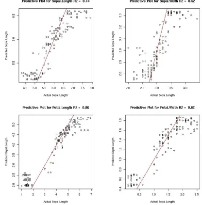
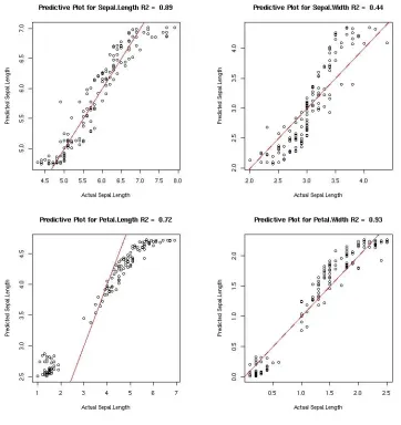
(56) AA-RF has the advantage of observing the group structure within the response and the predictor variables, which results in a significantly clearer proximity image with the three groups being obvious along the diagonal (Figure 8). This is translated into a clear MDS representation for AA-RF (Figure 8) where the groups ‘vericolor’ (2) and ‘virginica’ (3) are less overlapping than in unsupervised random forests. Furthermore, an analysis of the predictive performance of the AA-RF can be observed (Figure 9) to assess the accuracy of the groups found in the MDS plots. Figure 8: A comparison between the unsupervised random forest and AA-RF proximities. The proximity matrices have been re-ordered by the known iris groups: (1) Setosa, (2) Vericolor, (3) Virginica. Yellow represents a high count between the observations, red a low count.. 55.

(57) Figure 9: AA-RF predictive performance with predictions on the y-axis and actual variables on the x-axis and a reference line running through y = x. The multivariate R2 = 0.97 and the individual variable R2s are printed in the titles of each plot.. 56.

No results found