Flow structure of subcooled boiling flow in an internally heated annulus

Flow structure of subcooled boiling flow in an internally heated annulus

Rong Situ a, Takashi Hibiki a, b, *, Xiaodong Sun a, Ye Mi a,1, Mamoru Ishii a

a

School of Nuclear Engineering, Purdue University, 400 Central Drive, West Lafayette,

IN 47907-2017, USA

b

Research Reactor Institute, Kyoto University, Kumatori, Sennan, Osaka 590-0494,

Japan

1

Current address: En'Urga Inc., 1291 Cumberland Avenue, West Lafayette, IN 47906,

USA

* Corresponding author: Tel: +81-724-51-2373, Fax: +81-724-51-2461, Email:

[email protected]

Abstract---Local measurements of flow parameters were performed for vertical

upward subcooled boiling flows in an internally heated annulus. The annulus channel

consisted of an inner heater rod with a diameter of 19.1 mm and an outer round pipe

with an inner diameter of 38.1 mm, and the hydraulic equivalent diameter was 19.1 mm.

The double-sensor conductivity probe method was used for measuring local void

fraction, interfacial area concentration, and interfacial velocity. A total of 11 data were

acquired consisting of four inlet liquid velocities, 0.500, 0.664, 0.987 and1.22 m/s and

two inlet liquid temperatures, 95.0 and 98.0 °C. The constitutive equations for

distribution parameter and drift velocity in the drift-flux model, and the semi-theoretical

correlation for Sauter mean diameter, namely, interfacial area concentration, which

were proposed previously, were validated by local flow parameters obtained in the

Key Words: Void fraction, Interfacial area concentration, Drift-flux model, Subcooled boiling flow; Multiphase flow; Internally heated annulus.

Nomenclature

A coefficient

ai interfacial area concentration

C0 distribution parameter

Db,max maximum bubble diameter

Drod diameter of inner rod

DH hydraulic equivalent diameter

DSm Sauter mean diameter

G mass flux

g gravitational acceleration

hfg latent heat

j mixture volumetric flux

jg superficial gas velocity

jf superficial liquid velocity

LH heated length

Lo Laplace length

Nsub subcooling number

NZu Zuber number

n exponent

P pressure

R radius of outer round pipe

R0 radius of inner rod

Re Reynolds number

Ref Reynolds number of liquid phase

Tin inlet temperature

r radial coordinate

Vgj void fraction-weighted mean drift velocity

vf,in inlet fluid velocity

vg interfacial velocity

vr relative velocity

vgj local drift velocity

We Weber number

xeq. thermal equilibrium quality

z axial coordinate

zh heated length

Greek symbols

α

∆hsub subcooling enthalpy

∆Tbulk difference between bulk liquid temperature and saturation temperature

∆

ρ

ε

ν

ρ

ρ

σ

Mathematical symbols

< > area-averaged quantity

<< >> void fraction weighted cross-sectional area-averaged quantity

～ non-dimensional quantity

1. Introduction

The capability to predict the void fraction and the interfacial area concentration

in subcooled boiling region is of considerable interest to boiling water reactor (BWR)

safety. This is because the void fraction significantly affects the reactor power and the

interfacial area concentration is one of the important parameters that determine the heat

transfer capability and the possible occurrence of critical heat flux. The existence of

the thermodynamic non-equilibrium between the phases complicates the analysis of the

subcooled boiling flow. The extensive literature reviews on subcooled boiling flow

researches were performed by Rogers and Li [1], Lee and Bankoff [2], and the present

authors [3]. The literature reviews covered both correlations and phenomenological

models and attempted to point out the major assumptions and methods applied to

developing these models. From the literature reviews, it has turned out that most

existing models or correlations are applicable only to limited experimental conditions.

It can also be seen that there is limited local data and no local data concerning

is desirable to establish a database of local interfacial parameters. It is also required to

develop reliable constitutive models for broad subcooled boiling conditions.

The purpose of this study is the continued enhancement of the safety of the

current generation of BWRs. In this study, local measurements of two-phase flow

parameters such as void fraction, interfacial area concentration and interfacial velocity

are conducted in subcooled boiling flows in an experimental loop. The extensive

discussions are performed to examine the dependence of inlet liquid temperature, heat

flux and inlet liquid velocity on local flow parameters. The obtained data are also used

for evaluating the applicability of existing drift-flux model and interfacial area

correlation to subcooled boiling flow.

2. Experimental

An experimental facility was designed to measure the relevant two-phase

parameters necessary for developing constitutive models for the two-fluid model in

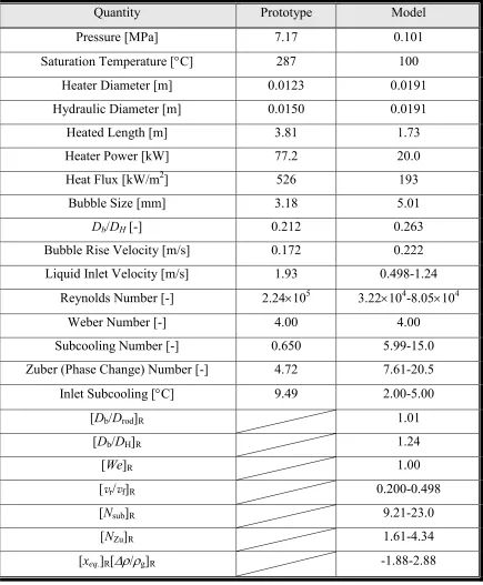
subcooled boiling. It was scaled to a prototypic BWR based on scaling criteria for

geometric, hydrodynamic, and thermal similarities [3]. The scaling criteria used to

design the test loop are detailed in Appendix. The experimental facility,

instrumentation, and data acquisition system are briefly described in this section.

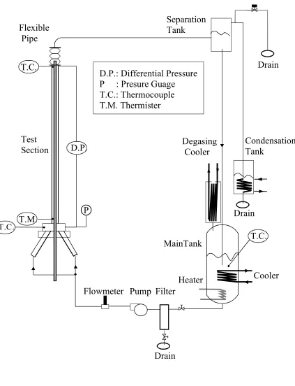
Figure 1 shows the experimental facility layout. The water supply is held in

the holding tank. The tank is open to the atmosphere through a heat exchanger

mounted to the top to prevent explosion or collapse and to degas from the water.

There is a cartridge heater inside the tank to heat the water and maintain the inlet water

temperature. A cooling line runs inside the tank to provide control of the inlet

positive displacement, eccentric screw pump, capable of providing a constant head with

minimum pressure oscillation. The water, which flows through a magnetic flow meter,

is divided into four separate flows and can then be injected into the test section. The

test section is an annular geometry that is formed by a clear polycarbonate pipe on the

outside and a cartridge heater on the inside. The test section is 38.1 mm inner diameter

and has a 3.18mm wall thickness. The overall length of the heater is 2670 mm and has

a 19.1 mm outer diameter. The heated section of the heater rod is 1730 mm long.

The heater rod has one thermocouple that is connected to the process controller to

provide feedback control. A pressure tap and thermocouple are placed at the inlet and

exit of the test section. A differential pressure cell is connected between the inlet and

outlet pressure taps. The two-phase mixture flows out of the test section to a separator

tank and the vapor phase is drained away. The water is returned to the holding tank.

There are several operation limits about the experimental loop that should be noted.

The limits are the flow rate of the liquid (143-2010 kg/(m2s) at 100 °C), the maximum

heat flux (0.193 MW/m2), the maximum cooling capacity (29 kW), and the inlet

subcooling (2.2-26 °C).

There are several K-type thermocouples used in the experimental loop. The

uncorrected error of these thermocouples is ±2.2 °C. A thermocouple measures the

temperature in the main tank. There are two thermocouples inserted into the inlet and

outlet flanges of the test section. Finally, there is a thermocouple inside the heater rod

to provide a feedback to the heater controller. A magnetic flow meter is used to

measure the average fluid flow rate entering the test section. The magnetic flow meter

has an accuracy of ±1 %. The differential pressure between the inlet and outlet of the

zero and span inaccuracy for this differential pressure cell is ±0.4 % of span. Silicon-controlled rectifier (SCR) is used to control the heat flux. The SCR uses

zero-voltage-switching that controls the load by controlling the number of completed

sine waves. Because only whole sine waves are used and the power is switched when

the sine wave crosses zero, there exists minimal radio frequency interference.

The double point electrical conductivity probe is used to make the two-phase

parameter measurements including void fraction, interfacial area concentration, and

interfacial velocity. The diameter of the probe tip is less than 0.002 mm. The double

sensor probe methodology was detailed in our previous paper [4], and the measurement

accuracies for void fraction, interfacial area concentration and interfacial velocity were

estimated to be ±12.8, ±6.95, and ±12.9 %, respectively [4]. There is an electrical

double-sensor conductivity probe at the axial location of zh/DH =52.6. The radial

distributions of the flow parameters were obtained by traversing the double sensor probe

along the radial direction. The radial locations measured by the probe are from

r/(R-R0) = 0.05 to 0.95, where r/(R-R0) = 0 and 1 correspond to the surface of the inner

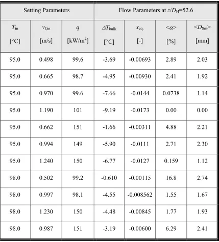
rod and outer pipe, respectively. The flow conditions in this experiment are tabulated

in Table 1.

3. Results and discussion

3.1. Measured flow parameters

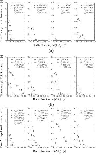
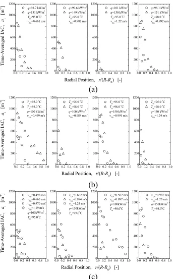
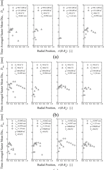
Figures 2-5 show the radial distributions of local void fraction, interfacial area

concentration, interfacial velocity, and bubble Sauter mean diameter, respectively. In

each figure, upper (a), middle (b), and lower (c) figures show the radial distributions of

and inlet liquid velocity, respectively.

As expected in subcooled boiling flow, a sharp peaking close to the heater

surface is observed in the void fraction distributions, see Fig.2. The void fraction

reaches maximum around r/(R-R0) = 0.1, i.e., 0.95 mm from the heater surface. Figure

5 shows that maximum local bubble diameters are around 2 mm. Thus, the peak

position of the void fraction roughly corresponds to the maximum bubble radius.

Since the bulk subcooling increases along the radial direction, the bubbles collapse and

the void fraction drops along the radial direction sharply. Figure 2 shows the

dependence of void fraction profile on thermal and flow parameters. As the heat flux

increases, the void fraction not only increases in value, but also propagates along the

radial direction, see Fig.2(a). The effect of increasing inlet temperature or decreasing

inlet liquid velocity has the similar consequence, see Fig.2(b) and (c), respectively.

Figure 2 also indicates the existence of a bubble layer in subcooled boiling, that is, the

flow can be characterized as two distinctive flow regions, boiling two-phase (bubble

layer) region and liquid single-phase region [5]. As heat flux increases, inlet

temperature increases, or inlet liquid velocity decreases, the bubble layer thickness

increases.

As shown in Fig.3, the radial distribution of interfacial area concentration

exhibits the similar behavior to that of void fraction. The local interfacial area

concentration reaches the peak around r/(R-R0) = 0.1, and then drops significantly along

the radial direction. The effects of thermal and flow parameters on the interfacial area

concentration are also similar to those on the void fraction, that is, the interfacial area

concentration increases as heat flux increases, or inlet temperature increases, or inlet

As shown in Fig.4, for most of the experimental conditions, the local interfacial

velocity profiles are found to be almost flat in the region where the radial location is

roughly smaller than the local bubble Sauter mean diameter, namely, r ≤ DSm,max.

Since the bubbles in the region are expected to slide on the heater surface, the flat

interfacial velocity profile in the bubble-layer region may mainly be due to the sliding

bubbles on the heater surface. For r > DSm,max, the interfacial velocity gradually

increase along the radial direction, and may reach its maximum value around the

channel center. The inlet liquid Reynolds numbers varies in the experiments from

28,870 to 70,260, which means that the flows are essentially turbulent flow. Thus, the

liquid velocity profile is expected to be quite flat around the channel center. Therefore,

the increase in the interfacial velocity along the radial direction around the channel

center may not be so significant.

The flow and thermal parameters affect the distribution of interfacial velocity

profile. Figures 4(a) and 4(b) indicates that the increase of the heat flux increases the

interfacial velocity and the increase of the inlet liquid temperature increases the

interfacial velocity, respectively. The increase of the heat flux or the inlet liquid

temperature increases the void fraction, resulting in the liquid velocity. Thus, the

increase of the interfacial velocity may mainly be attributed to the increased void

fraction. Figure 4 (c) shows the dependence of the inlet liquid flow rate on the

interfacial velocity. Unlike the dependence of the heat flux or the inlet liquid

temperature on the interfacial velocity, the effect of the inlet liquid velocity on the

interfacial velocity may not be clear in the vicinity of the heater surface in some

experimental conditions. The increase in the liquid velocity certainly tends to increase

velocity and the relative velocity between phases. On the other hands, the increase in

the liquid velocity keeping the heat flux and the inlet liquid velocity constant decreases

the void fraction, see Fig.2(c). Thus, the systematic effect of the liquid velocity on the

interfacial velocity is not obtained particularly in the vicinity of the heater surface.

As expected in subcooled boiling flow, a sharp increase close to the heater

surface is observed in the bubble Sauter mean diameter distributions, see Fig.5. At

low void fraction conditions, the distribution profile of the bubble diameter along the

radial direction is similar to that of the void fraction. This indicates that bubbles

collapse in the subcooled bulk region due to high liquid subcooling. On the other hand,

at higher void fraction condition, such as the condition with Tin = 98.0°C, q = 100

kW/m2, and vf,in=0.499 m/s, the void fraction keeps dropping along the radial direction

even at the outer half of the channel. However, the bubble diameter is still about 2 mm

even in the vicinity of the outer channel wall. This suggests that the bulk temperature

is around saturate temperature and thus bubbles would not collapse. The effects of

flow and thermal parameters on the radial profile of Sauter-mean diameter is similar to

those on the void fraction profile, that is, as heat flux increases, or inlet temperature

increases, or inlet liquid velocity decreases, the Sauter-mean diameter will increase.

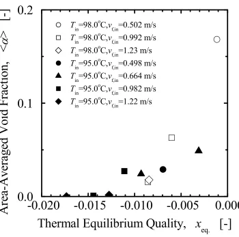
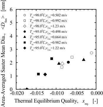
Figures 6 and 7 show the dependence of the area-averaged void fraction on the

thermal equilibrium quality and the dependence of the area-averaged Sauter-mean

diameter on the thermal equilibrium quality, respectively. These figures imply that the

area-averaged void fraction and bubble Sauter mean diameter can closely be related to

the thermal equilibrium quality. When the thermal equilibrium quality is less than

–0.013, the void fraction is negligibly small, see Fig.6. As the thermal equilibrium

quality is -0.0012. When the thermal equilibrium quality is less than -0.017, the

bubble Sauter mean diameter is almost zero, see Fig.7. As the thermal equilibrium

quality increases, the bubble diameter increases gradually, and it reaches about 3 mm

when the thermal equilibrium quality is 0.

3.2. Constitutive equations of void fraction and interfacial area concentration

The void fraction and interfacial area concentration are two fundamental

geometrical parameters in a bubbly two-phase flow. The void fraction expresses the

phase distribution and is a required parameter for hydrodynamic and thermal design in

various industrial processes. On the other hand, the interfacial area concentration

describes available area for the interfacial transfer of mass, momentum and energy, and

is a required parameter for a two-fluid model formulation. Various transfer

mechanisms between phases depend on the two-phase interfacial structures. Therefore,

an accurate knowledge of these parameters is necessary for any two-phase flow analyses.

This fact can further be substantiated with respect to two-phase flow formulation. In

what follows, the constitutive equations for distribution parameter and drift velocity in

the drift-flux model, and the semi-theoretical correlation for Sauter mean diameter

namely interfacial area concentration, which were proposed previously, were validated

by area-averaged flow parameters obtained by integrating local flow parameters over

the flow channel.

3.2.1 Constitutive equation of void fraction---Drift-flux model

The drift-flux model is one of the most practical and accurate models for

distribution parameter and drift velocity in the drift-flux model to subcooled boiling

flow will be examined by the data obtained in this study. The one-dimensional

drift-flux model is given by [6]

gj gj

g g

g C j V

v j

j j j

v

v = = = + = ₀ +

α

α

α

α

α

α

α

, (1)

where vgj is the drift velocity of a gas phase defined as the velocity of the gas phase with

respect to the volume center to the mixture. The distribution parameter, C0, and the

void-fraction-weighted mean drift velocity, Vgj, are defined as

j j C

α

α

≡

0 and

α

α

gj

v

V = . (2)

Ishii [7] developed the constitutive equation of the distribution parameter in

developing flow due to boiling in a round pipe as:

(

ρ

ρ

)

(

)

0 12 02 1

−

− −

= . . e

C _{g f} , (3)

Recently, Hibiki et al. [5] successfully derived the constitutive equation of the

distribution parameter in developing flow due to boiling in an internally-heated annuls

from Eq.(3) by considering the difference in the channel geometry as:

(

)

(

)

0 1.2 0.2 g f 1 exp 3.12

C = − ρ ρ  − − α 

 . (4)

On the other hand, Ishii [7] developed the constitutive equation of the void-fraction-weighted mean drift velocity in bubbly flow regime as:

(

)

1

2 1

2 .

f gj

g

V

α

ρ

ρ

∆

σ

    

  

From Eqs.(1), (4) and (5), the one-dimensional drift flux model can be recast in the following form.

(

)

{

(

)

}

(

)

(

)

{

(

)

}

1 4

1.75 0.212

2 0.212

1.2 0.2 1 exp 3.12 2 1

1 1.2 0.2 1 exp 3.12

g f f

f g

g f

g j

j

ρ σ

ρ ρ α α

ρ

α ρ ρ α

_∆ 

− − − + _ _ −

 

=

− − − −

(6)

The above equation indicates that the superficial gas velocity is a function of the void fraction at a fixed superficial liquid velocity in a certain fluid system.

The distribution parameter and the drift velocity can be determined from Eq.(2) experimentally, provided that local void fraction and gas and liquid velocities are available. In this study, since no local liquid velocity data are available, the profile of the mixture volumetric flux in the estimation of the distribution parameter using measured local void fraction is approximated by

    

  

− − − +

=

n

R R

r j

n n j

0

2 1 1 1

. (7)

Since the profile of mixture volumetric flux is expected to be more or less a power-law profile in a turbulent flow, the approximated profile of the mixture volumetric flux may not affect the estimation of the distribution parameter significantly [4, 5]. This means that the void fraction profile is a dominant parameter to determine the distribution parameter in a turbulent flow. Thus, n is assumed to be 7 in this study [5].

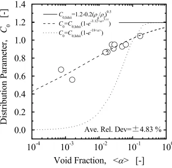
the experimentally determined distribution parameters, the asymptotic value of the distribution parameter at <α>=1 calculated by Eq.(3), the distribution parameter

calculated by Eq.(4), and the distribution parameter calculated by Eq.(3), respectively. As can be seen from Fig.8, Eq.(4) can reproduce the dependence of the distribution parameter on the void fraction properly. This may be attributed to the proper modeling of the distribution parameter, Eq.(4), by considering the flow developing process in subcooled boiling flow [5]. The average relative deviation between Eq.(4) and the distribution parameters estimated experimentally is estimated to be ±4.83 %.

In Fig.9, the superficial gas velocities are plotted against the void fractions as a parameter of the superficial liquid velocity. The superficial liquid velocity is calculated by

(

)

f g g f

j = G−ρ j ρ . (8)

drift velocity should be examined separately by local flow data of gas and liquid phases to be measured in a future study.

The constitutive equation of the distribution parameter, Eq.(4), and the drift-flux model, Eq.(6) are also evaluated by existing data. Lee et al. [8] conducted local flow measurements of subcooled water boiling flow in an internally heated annulus. The outer diameter of a heated inner pipe and the inner diameter of an outer pipe were 19.0 mm and 37.5 mm, respectively. In their experiment, a total of 18 data sets were acquired consisting of the mass flux, 476-1061 kg/m2s, the heat flux, 114.8-320.4 kW/m2, and the inlet subcooling, 11.5-21.3 °C. Equations (4) and (6) can predict the distribution parameters and the superficial gas velocities within an average relative derivation of ±9.73 % and ±4.20 %, respectively. Roy et al. [9] also performed local flow measurements of subcooled R-113 boiling flow in an internally heated annulus. The outer diameter of a heated inner pipe and the inner diameter of an outer pipe were 15.9 mm and 38.1 mm, respectively. The experiments were carried out at the mass flux, 579 and 801 kg/m2s, the heat flux, 79.4-126.0 kW/m2, and the wall temperature 95-102 °C. A total of 7 complete data sets to calculate the distribution parameter and the other flow parameters are available in the paper. Equations (4) and (6) can predict the distribution parameters and the superficial gas velocities within an average relative derivation of ±27.5 % and ±10.7 %, respectively. Although the available data supports the validity of Eqs.(4) and (6), extensive efforts to take local flow data should be encouraged to evaluate the constitutive equations in a future study.

3.2.2 Constitutive equation of interfacial area concentration and bubble diameter

interfacial area concentration under steady fully-developed adiabatic bubbly flow conditions based on the interfacial area transport equation as follows:

239 0 335

0

02

3 . .

i Re

~ o

L~ .

a~ = α or D~_Sm =1.99L~o−0.335R~e−0.239 (9)

where a~_i ≡ a_i Lo ,

ρ ∆ σ g

Lo≡ ,

H

D Lo o

L~ ≡ ,

(

)

f

Lo Lo e

R~

ν ε 13 13

≡ , and

(

)

Lo D Lo

a

D~ i Sm

Sm ≡ =

α 6

. The energy dissipation rate per unit mass in Eq.(9) is approximated by [8]

(

)

{

(

)

}

F m

f

g ARe

dz dP j

ARe j

g _ − −

     − + −

= exp 1 exp

ρ

ε , (10)

where g, A, Ref, ρm, and (-dP/dz)F refer to the gravitational acceleration, a coefficient (= 0.0005839), Reynolds number of the liquid phase defined by <jf>DH/νf, the mixture density, and the pressure loss per unit length due to friction, respectively. Although the applicability of Eq.(9) to developing flows was also confirmed experimentally [10], the applicability of Eq.(9) to subcooled boiling flow has not been examined because of very limited available data. It should be noted here that the heat flux does not appear in Eq.(9) explicitly. However, since the superficial gas and liquid velocities depend on the heat flux, the bubble diameter is certainly dependent on the heat flux.

given by Eq.(9) can be applicable to subcooled boiling flow in an internally heated annulus.

The constitutive equation of the bubble Sauter mean diameter, Eq.(9) is also evaluated by the R-113 data taken by Roy et al. [9].existing data. Only one complete datum to calculate the bubble Sauter mean diameter and the other flow parameters is available at the mass velocity of 801 kg/m2s, the heat flux of 115.8 kW/m2, and the inlet R-113 temperature of 43.0 °C. Equation (9) can predict the bubble Sauter mean diameter with a relative derivation of ±25.0 %. Although the available datum supports the validity of Eq.(9), extensive efforts to take local flow data should be encouraged to evaluate the constitutive equation in a future study.

4. Conclusions

Local measurements of flow parameters were performed for vertical upward subcooled boiling flows in an internally heated annulus. The annulus channel consisted of an inner heater rod with a diameter of 19.1 mm and an outer round pipe with an inner diameter of 38.1 mm, and the hydraulic equivalent diameter was 19.1 mm. The double-sensor conductivity probe method was used for measuring local void fraction, interfacial area concentration, and interfacial velocity. The obtained results are summarized below.

(1) A total of 11 data were acquired consisting of four inlet liquid velocities, 0.500, 0.664, 0.987 and1.22 m/s and two inlet liquid temperatures, 95.0 and 98.0 °C.

temperature, and the inlet liquid velocity were discussed in detail.

(3) The constitutive equation for the distribution parameter in the drift-flux model proposed previously was evaluated by local flow parameters obtained in the experiment. The constitutive equation for the distribution parameter could predict the experimentally determined distribution parameter within an average relative deviation of ±4.83 %. The drift flux model with the validated constitutive equations for the distribution parameter could also predict the experimental data within an average relative deviation of ±6.92 %.

(4) The semi-theoretical correlation for Sauter mean diameter, namely, interfacial area concentration proposed previously was validated by local flow parameters obtained in the experiment. The correlation for Sauter mean diameter could predict the measured Sauter mean diameter within an average relative deviation of ±23.9 %.

Acknowledgments

The research project was supported by the Tokyo Electric Power Company (TEPCO). The authors would like to express their sincere appreciation for the support and guidance from Dr. Mori of the TEPCO.

Appendix A

the inlet to the saturation temperature 287 °C. The prototypic conditions in the BWR core is simulated by an atmospheric pressure loop using water as the coolant based on the scaling method, which provides similar geometric, hydrodynamic, and thermal characteristics as those found in the prototype.

The non-dimensional parameters specifying similar hydraulic and thermal characteristics of the flow are obtained from the scaling method. These non-dimensional parameters include the Reynolds number and the Weber number. However, it is almost impossible to satisfy all the flow characteristics because each flow property depends on the fluid properties and the fluid properties are different. This is particularly true when the flow has more than one phase such as a vapor/liquid flow. For the vapor/liquid flow the geometrical similarity is important, i.e. the relative size of the bubble to the channel structure. A large deviation of the geometrical conditions from the flow in the prototype induces a significant change in the vapor phase distribution and could even results in a different flow regime. Therefore, the geometrical similarity is used as the first scaling criteria.

Geometrical similarity

The ratio of the bubble diameter to the heating rod diameter should be scaled as:

1

b rod R

D D é ù ê _{ú =} ê ú ë û

. (A.1)

Similarly the ratio of the bubble diameter to the hydraulic diameter should be scaled as:

1

b H R

D D é ù ê _{ú =} ê ú ë û

, (A.2)

where the subscript R denotes the ratio of the value for a model to that of the prototype.

for model for prototype

m R

p

y y

y

y y

º = . (A.3)

Both criteria, Eqs.(A-1) and (A-2) are effective in the bubble layer development for subcooled convection boiling flow. To estimate the heating rod diameter and the hydraulic diameter in the model, we may approximate the bubble diameter as:

2

,max b b

D

D » , (A.4)

where Db,max is the maximum distorted bubble limit given by [15]:

4

,max b

D

g s D r

= . (A.5)

Hydrodynamic similarity

The ratio of the relative velocity to the liquid velocity should be scaled as:

1

r f _R

v v

é ù ê ú = ê ú ê ú ë û

. (A.6)

velocity, vr, as [15]: 1 4 2 2 r f g

v s D r

r æ ö_÷

ç _÷

ç

» _{ç ÷}

÷ ÷ ççè ø

. (A.7)

Thermal similarity

Subcooled number, Nsub, and Zuber number (phase change number), NZu, play an important role in the thermal similarity criteria. The subcooled number is the ratio of the subcooling to the latent heat as:

sub sub fg g h N h

D D r

r æ ö_÷ ç _÷ ç

= _{ç ÷}

÷ ÷ ççè ø

, (A.8)

where ∆hsub and hfg are the subcooling enthalpy and the latent heat, respectively. The

Zuber number is the ratio of the heat flux used for phase change over the inlet subcooling as:

4

, h Zu

H f in fg f g

q L N

D v h

D r r r æ ö ÷ ç _÷ ç

= _{ç ÷}

÷ ÷ ççè ø

, (A.9)

where Lh is the heated length.

From the steady state energy equation balanced over the heated section using a control volume analysis, Nsub and NZu are related by:

.

eq Zu sub g

x N N

D r r æ ö

÷ ç _÷

ç _÷ =

-ç _÷÷ ççè ø

. (A.10)

Therefore, the similarity of the subcooling and Zuber numbers yields:

1

. eq R

g _R

x D r

r

é ù

ê ú

é ù ₌

ë û ê ú

ê ú

ë û

. (A.11)

Some of the important scaling criteria are highlighted as described above, and the detailed discussions on the scaling criteria are found in the previous papers [11-15]. The loop geometry and the thermal-hydraulic conditions in the prototypic BWR and the scaled model are tabulated in Table A-1. In the test loop used in the present experiment, the geometrical similarity is almost preserved, but hydrodynamic and thermal similarities are not completely preserved due to the limited capability of the test equipment. The typical ranges of the similarity parameters covered in the present experiment are also tabulated in Table A-1. Thus, since the geometrical similarity, namely the bubble migration characteristics is preserved in the present experiment, the obtained data would provide the information on more general basic flow characteristics in the channel of the BWR core rather than that at the operating condition of the BWR.

References

[1] J. T. Rogers and J. Li, Prediction of the onset of significant void in flow boiling of water, ASME Paper HTD-217, Fundamentals of Subcooled Flow Boiling (1992) 41-52.

[2] S. C. Lee and S. G. Bankoff, A comparison of predictive models for the onset of significant void at low pressures in forced-convection subcooled boiling, KSME Int. J. 12 (1998) 504-513.

[3] M. D. Bartel, M. Ishii, T. Masukawa, Y. Mi, R. Situ, Interfacial area measurements in subcooled flow boiling, Nucl. Eng. Des. 210 (2001) 135-155. [4] T. Hibiki, R. Situ, Y. Mi, M. Ishii, Local flow measurements of vertical upward

formulation of one-dimensional interfacial area transport equation in subcooled boiling two-phase flow, Int. J. Heat Mass Transfer 46 (2003) 1409-1423.

[6] N. Zuber, J. A. Findlay, Average volumetric concentration in two-phase flow systems, J. Heat Transfer 87 (1965) 453-468.

[7] M. Ishii, One-dimensional drift-flux model and constitutive equations for relative motion between phases in various two-phase flow regimes, ANL-77-47, USA, 1977.

[8] T. H. Lee, G. C. Park, D. J. Lee, Local flow characteristics of subcooled boiling flow of water in a vertical concentric annulus, Int. J. Multiphase Flow 28 (2002) 1351-1368.

[9] R. P. Roy, V. Velidandla, S. P. Kalra, P. Peturaud, Local measurements in the two-phase region of turbulent subcooled boiling flow, J. Heat Transfer 116 (1994) 660-669.

[10] T. Hibiki, M. Ishii, Interfacial area concentration of bubbly flow systems, Chem. Eng. Sci. 45 (2002) 707-721.

[11] M. Ishii, I. Kataoka, “Scaling laws for thermal-hydraulic system under single phase and two-phase natural circulation,” Nucl. Eng. Des. 81 (1984) 411-425. [12] G. Kocamustafaogullari, M. Ishii, “Scaling criteria for two-phase flow loop and

their application to conceptual 2 × 4 simulation loop design,” Nucl. Technol. 65 (1984) 146-160.

[13] M. Ishii, H.C. No, G. Zhang, F. Eltwila, “Stepwise integral scaling methods for severe accident analysis and it's application to corium dispersion in direct containment heating,” Nucl. Eng. Des. 151 (1994) 223-234.

W. Wang, H. Pokharna, V. H. Ransom, R. Viskanta, J. T. Han, “The three-level scaling approach with application to the Purdue University multi-dimensional integral test assembly (PUMA),” Nucl. Eng. Des. 186 (1998) 177-212.

[15] M. Ishii and N. Zuber, “Drag coefficient and relative velocity in bubbly, droplet or particulate flows,” AIChE J. 25 (1979) 843-855.

Captions of Figures

Fig.1. Schematic diagram of experimental loop.

Fig.2. Local void fraction profiles as a parameter of (a) heat flux, (b) inlet liquid temperature, and (c) inlet liquid velocity.

Fig.3. Local interfacial area concentration profiles as a parameter of (a) heat flux, (b) inlet liquid temperature, and (c) inlet liquid velocity.

Fig.4. Local interfacial velocity profiles as a parameter of (a) heat flux, (b) inlet liquid temperature, and (c) inlet liquid velocity.

Fig.5. Local Sauter mean diameter profiles as a parameter of (a) heat flux, (b) inlet liquid temperature, and (c) inlet liquid velocity.

Fig.6. Dependence of area-averaged void fraction on thermal equilibrium quality. Fig.7. Dependence of area-averaged bubble Sauter mean diameter on thermal

equilibrium quality.

Fig.8. Dependence of distribution parameter on void fraction in subcooled boiling flow.

Fig.10. Comparison of semi-theoretical correlation for Sauter mean diameter with experimental data.

Table 1. Flow conditions in this experiment.

Setting Parameters Flow Parameters at z/DH=52.6

Tin [°C]

vf,in [m/s]

q

[kW/m2]

∆Tbulk [°C]

xeq. [-]

<α>

[%]

<DSm> [mm]

95.0 0.498 99.6 -3.69 -0.00693 2.89 2.03

95.0 0.665 98.7 -4.95 -0.00930 2.41 1.92

95.0 0.970 99.6 -7.66 -0.0144 0.0738 1.14

95.0 1.190 101 -9.19 -0.0173 0.00 0.00

95.0 0.662 151 -1.66 -0.00311 4.88 2.21

95.0 0.994 149 -5.90 -0.0111 2.71 2.30

95.0 1.240 150 -6.77 -0.0127 0.159 1.12

98.0 0.502 99.2 -0.610 -0.00115 16.8 2.74

98.0 0.997 98.1 -4.55 -0.008562 1.55 1.67

98.0 1.230 150 -4.48 -0.00845 1.77 1.93

Table A.1. Prototypic BWR conditions and experimental conditions in the present experiment.

Quantity Prototype Model

Pressure [MPa] 7.17 0.101

Saturation Temperature [°C] 287 100 Heater Diameter [m] 0.0123 0.0191 Hydraulic Diameter [m] 0.0150 0.0191

Heated Length [m] 3.81 1.73

Heater Power [kW] 77.2 20.0

Heat Flux [kW/m2] 526 193

Bubble Size [mm] 3.18 5.01

Db/DH [-] 0.212 0.263

Bubble Rise Velocity [m/s] 0.172 0.222 Liquid Inlet Velocity [m/s] 1.93 0.498-1.24

Reynolds Number [-] 2.24×105 3.22×104-8.05×104

Weber Number [-] 4.00 4.00

Subcooling Number [-] 0.650 5.99-15.0 Zuber (Phase Change) Number [-] 4.72 7.61-20.5 Inlet Subcooling [°C] 9.49 2.00-5.00

[Db/Drod]R 1.01

[Db/DH]R 1.24

[We]R 1.00

[v_r/v_{f]R 0.200-0.498}

[Nsub]R 9.21-23.0

[NZu]R 1.61-4.34

Fig. 1

Heater

Cooler

Flexible

Pipe

Separation

Tank

MainTank

Flowmeter Pump

Heater

Rod

Height

Adjuster

Test

Section

T.C.

Filter

Drain

Degasing

Cooler

Drain

Drain

T.M.

T.C.

T.C.

Condensation

Tank

D.P.

P

Fig. 2 0.0 0.2 0.4 0.6 0.8 1.0

0.0 0.1 0.2 0.3 0.4 0.5 0.6

q=99.6 kW/m2

q=149 kW/m2

Tin=95.0

o

C

v_f,in=0.982 m/s

0.0 0.2 0.4 0.6 0.8 1.0 0.0 0.1 0.2 0.3 0.4 0.5 0.6 T im e-A v er ag ed V o id F ra ct io n , α [ -]

q=98.7 kW/m2

q=151 kW/m2

Tin=95.0

o

C

v_f,in=0.661 m/s

0.0 0.2 0.4 0.6 0.8 1.0 0.0 0.1 0.2 0.3 0.4 0.5 0.6

q=98.1 kW/m2

q=151 kW/m2

Tin=98.0

o

C

v_f,in=0.992 m/s

Radial Position, r/(R-R

0) [-] 0.0 0.2 0.4 0.6 0.8 1.0 0.0 0.1 0.2 0.3 0.4 0.5 0.6

q=101 kW/m2

q=150 kW/m2

Tin=95.0

o

C

v_f,in=1.22 m/s

0.0 0.2 0.4 0.6 0.8 1.0 0.0 0.1 0.2 0.3 0.4 0.5 0.6

T_in=95.0 o

C

Tin=98.0

o

C

q=100 kW/m2

vf,in=0.499 m/s

T im e-A v er ag ed V o id F ra ct io n , α [ -]

0.0 0.2 0.4 0.6 0.8 1.0 0.0 0.1 0.2 0.3 0.4 0.5 0.6

T_in=95.0 o

C

Tin=98.0

o

C

q=100 kW/m2

vf,in=0.984 m/s

0.0 0.2 0.4 0.6 0.8 1.0 0.0 0.1 0.2 0.3 0.4 0.5 0.6

T_in=95.0 o

C

Tin=98.0

o

C

q=150 kW/m2

vf,in=0.991 m/s

Radial Position, r/(R-R

0) [-]

0.0 0.2 0.4 0.6 0.8 1.0 0.0 0.1 0.2 0.3 0.4 0.5 0.6

T_in=95.0 o

C

Tin=98.0

o

C

q=150 kW/m2

vf,in=1.24 m/s

0.0 0.2 0.4 0.6 0.8 1.0 0.0 0.1 0.2 0.3 0.4 0.5 0.6

v_f,in=0.498 m/s

vf,in=0.665 m/s

v_f,in=0.970 m/s

vf,in=1.19 m/s

q=100kW/m2

Tin=95.0

o C T im e-A v er ag ed V o id F ra ct io n , α [ -]

0.0 0.2 0.4 0.6 0.8 1.0 0.0 0.1 0.2 0.3 0.4 0.5 0.6

v_f,in=0.662 m/s

vf,in=0.994 m/s

v_f,in=1.24 m/s

q=150kW/m2

T_in=95.0o

C

0.0 0.2 0.4 0.6 0.8 1.0 0.0 0.1 0.2 0.3 0.4 0.5 0.6

v_f,in=0.502 m/s

vf,in=0.997 m/s

q=100kW/m2

Tin=98.0

o

C

Radial Position, r/(R-R

0) [-]

0.0 0.2 0.4 0.6 0.8 1.0 0.0 0.1 0.2 0.3 0.4 0.5 0.6

v_f,in=0.987 m/s

vf,in=1.23 m/s

q=150kW/m2

Tin=98.0

o

C

(a)

(b)

Fig. 3 0.0 0.2 0.4 0.6 0.8 1.0

0 200 400 600 800 1000 1200

Radial Position, r/(R-R₀) [-]

q=99.6 kW/m2

q=149 kW/m2

Tin=95.0

o

C

vf,in=0.982 m/s

0.0 0.2 0.4 0.6 0.8 1.0 0 200 400 600 800 1000 1200 T im e-A v er ag ed I A C , a i [ m

-1 ] q=98.7 kW/m

2

q=151 kW/m2

Tin=95.0

o

C

vf,in=0.661 m/s

0.0 0.2 0.4 0.6 0.8 1.0 0 200 400 600 800 1000 1200

q=98.1 kW/m2

q=151 kW/m2

Tin=98.0

o

C

vf,in=0.992 m/s

0.0 0.2 0.4 0.6 0.8 1.0 0 200 400 600 800 1000 1200

q=101 kW/m2

q=150 kW/m2

Tin=95.0

o

C

vf,in=1.22 m/s

0.0 0.2 0.4 0.6 0.8 1.0 0 200 400 600 800 1000 1200

T_in=95.0 o

C

Tin=98.0

o

C

q=100 kW/m2

vf,in=0.499 m/s

T im e-A v er ag ed I A C , a i [ m -1 ]

0.0 0.2 0.4 0.6 0.8 1.0 0 200 400 600 800 1000 1200

T_in=95.0 o

C

Tin=98.0

o

C

q=100 kW/m2

vf,in=0.984 m/s

0.0 0.2 0.4 0.6 0.8 1.0 0 200 400 600 800 1000 1200

T_in=95.0 o

C

Tin=98.0

o

C

q=150 kW/m2

vf,in=0.991 m/s

Radial Position, r/(R-R

0) [-]

0.0 0.2 0.4 0.6 0.8 1.0 0 200 400 600 800 1000 1200

T_in=95.0 o

C

Tin=98.0

o

C

q=150 kW/m2

vf,in=1.24 m/s

0.0 0.2 0.4 0.6 0.8 1.0 0 200 400 600 800 1000 1200

vf,in=0.498 m/s

vf,in=0.665 m/s

v_f,in=0.970 m/s

v_f,in=1.19 m/s

q=100kW/m2

T_in=95.0o

C T im e-A v er ag ed I A C , a i [ m -1 ]

0.0 0.2 0.4 0.6 0.8 1.0 0 200 400 600 800 1000 1200

vf,in=0.662 m/s

vf,in=0.994 m/s

v_f,in=1.24 m/s

q=150kW/m2

Tin=95.0

o

C

0.0 0.2 0.4 0.6 0.8 1.0 0 200 400 600 800 1000 1200

vf,in=0.502 m/s

vf,in=0.997 m/s

q=100kW/m2

Tin=98.0

o

C

Radial Position, r/(R-R

0) [-]

0.0 0.2 0.4 0.6 0.8 1.0 0 200 400 600 800 1000 1200

vf,in=0.987 m/s

vf,in=1.23 m/s

q=150kW/m2

Tin=98.0

o

C

(a)

(b)

Fig.4 0.0 0.2 0.4 0.6 0.8 1.0

0.0 0.5 1.0 1.5 2.0 2.5

q=99.6 kW/m2

q=149 kW/m2

T_in=95.0 o

C

vf,in=0.982 m/s

0.0 0.2 0.4 0.6 0.8 1.0 0.0 0.5 1.0 1.5 2.0 2.5 T im e-A v er ag ed I n te rf ac ia l V el o ci ty , v g [ m /s

q=98.7 kW/m2

q=151 kW/m2

T_in=95.0 o

C

vf,in=0.661 m/s

0.0 0.2 0.4 0.6 0.8 1.0 0.0 0.5 1.0 1.5 2.0 2.5

q=98.1 kW/m2

q=151 kW/m2

T_in=98.0 o

C

vf,in=0.992 m/s

Radial Position, r/(R-R₀) [-]

0.0 0.2 0.4 0.6 0.8 1.0 0.0 0.5 1.0 1.5 2.0 2.5

q=101 kW/m2

q=150 kW/m2

T_in=95.0 o

C

vf,in=1.22 m/s

0.0 0.2 0.4 0.6 0.8 1.0 0.0 0.5 1.0 1.5 2.0 2.5

T_in=95.0 o

C

Tin=98.0

o

C

q=100 kW/m2

vf,in=0.499 m/s

T im e-A v er ag ed I n te rf ac ia l V el o ci ty , v g [ m /s ]

0.0 0.2 0.4 0.6 0.8 1.0 0.0 0.5 1.0 1.5 2.0 2.5

T_in=95.0 o

C

Tin=98.0

o

C

q=100 kW/m2

vf,in=0.984 m/s

0.0 0.2 0.4 0.6 0.8 1.0 0.0 0.5 1.0 1.5 2.0 2.5

T_in=95.0 o

C

Tin=98.0

o

C

q=150 kW/m2

vf,in=0.991 m/s

Radial Position, r/(R-R

0) [-]

0.0 0.2 0.4 0.6 0.8 1.0 0.0 0.5 1.0 1.5 2.0 2.5

T_in=95.0 o

C

Tin=98.0

o

C

q=150 kW/m2

vf,in=1.24 m/s

0.0 0.2 0.4 0.6 0.8 1.0 0.0 0.5 1.0 1.5 2.0 2.5

vf,in=0.498 m/s

v_f,in=0.665 m/s

vf,in=0.970 m/s

vf,in=1.19 m/s

q=100kW/m2

T_in=95.0o

C T im e-A v er ag ed I n te rf ac ia l V el o ci ty , v g [ m /s ]

0.0 0.2 0.4 0.6 0.8 1.0 0.0 0.5 1.0 1.5 2.0 2.5

vf,in=0.662 m/s

vf,in=0.994 m/s

vf,in=1.24 m/s

q=150kW/m2

Tin=95.0

o

C

0.0 0.2 0.4 0.6 0.8 1.0 0.0 0.5 1.0 1.5 2.0 2.5

vf,in=0.502 m/s

vf,in=0.997 m/s

q=100kW/m2

T_in=98.0o

C

Radial Position, r/(R-R₀) [-]

0.0 0.2 0.4 0.6 0.8 1.0 0.0 0.5 1.0 1.5 2.0 2.5

vf,in=0.987 m/s

vf,in=1.23 m/s

q=150kW/m2

Tin=98.0

o

C

(a)

(b)

Fig. 5 0.0 0.2 0.4 0.6 0.8 1.0

0 1 2 3 4 5 6

q=99.6 kW/m2

q=149 kW/m2

Tin=95.0

o

C

v_f,in=0.982 m/s

0.0 0.2 0.4 0.6 0.8 1.0 0 1 2 3 4 5 6 T im e-A v er ag ed S au te r M ea n D ia ., DS m [ m m

q=98.7 kW/m2

q=151 kW/m2

Tin=95.0

o

C

v_f,in=0.661 m/s

0.0 0.2 0.4 0.6 0.8 1.0 0 1 2 3 4 5 6

q=98.1 kW/m2

q=151 kW/m2

Tin=98.0

o

C

v_f,in=0.992 m/s

Radial Position, r/(R-R

0) [-] 0.0 0.2 0.4 0.6 0.8 1.0 0 1 2 3 4 5 6

q=101 kW/m2

q=150 kW/m2

Tin=95.0

o

C

v_f,in=1.22 m/s

0.0 0.2 0.4 0.6 0.8 1.0 0 1 2 3 4 5 6

Tin=95.0

o

C

Tin=98.0

o

C

q=100 kW/m2

vf,in=0.499 m/s

T im e-A v er ag ed S au te r M ea n D ia ., DS m [ m m ]

0.0 0.2 0.4 0.6 0.8 1.0 0 1 2 3 4 5 6

Tin=95.0

o

C

Tin=98.0

o

C

q=100 kW/m2

vf,in=0.984 m/s

0.0 0.2 0.4 0.6 0.8 1.0 0 1 2 3 4 5 6

Tin=95.0

o

C

Tin=98.0

o

C

q=150 kW/m2

vf,in=0.991 m/s

Radial Position, r/(R-R

0) [-]

0.0 0.2 0.4 0.6 0.8 1.0 0 1 2 3 4 5 6

Tin=95.0

o

C

Tin=98.0

o

C

q=150 kW/m2

vf,in=1.24 m/s

0.0 0.2 0.4 0.6 0.8 1.0 0 1 2 3 4 5 6

vf,in=0.498 m/s

vf,in=0.665 m/s

vf,in=0.970 m/s

v_f,in=1.19 m/s

q=100kW/m2

T_in=95.0o

C T im e-A v er ag ed S au te r M ea n D ia ., DS m [ m m ]

0.0 0.2 0.4 0.6 0.8 1.0 0 1 2 3 4 5 6

vf,in=0.662 m/s

vf,in=0.994 m/s

vf,in=1.24 m/s

q=150kW/m2

Tin=95.0

o

C

0.0 0.2 0.4 0.6 0.8 1.0 0 1 2 3 4 5 6

vf,in=0.502 m/s

vf,in=0.997 m/s

q=100kW/m2

Tin=98.0

o

C

Radial Position, r/(R-R₀) [-]

0.0 0.2 0.4 0.6 0.8 1.0 0 1 2 3 4 5 6

vf,in=0.987 m/s

vf,in=1.23 m/s

q=150kW/m2

Tin=98.0

o

C

(a)

(b)

Fig. 6

-0.020

-0.015

-0.010

-0.005

0.000

0.0

0.1

0.2

T

in=98.0

o

C,v

f,in=0.502 m/s

T

in=98.0

o

C,v

f,in=0.992 m/s

T_in=98.0oC,v_f,in=1.23 m/s

T_in=95.0oC,v_f,in=0.498 m/s

T_in=95.0oC,v_f,in=0.664 m/s

T_in=95.0oC,v_f,in=0.982 m/s

T_in=95.0oC,v_f,in=1.22 m/s

A

re

a-A

v

er

ag

ed

V

o

id

F

ra

ct

io

n

,

<

α

>

[

-]

Fig. 7

-0.020

-0.015

-0.010

-0.005

0.000

0

1

2

3

4

5

6

T_in=98.0oC,v_f,in=0.502 m/s

T_in=98.0oC,v_f,in=0.992 m/s

T_in=98.0oC,v_f,in=1.23 m/s

T_in=95.0oC,v_f,in=0.498 m/s

T

in=95.0

o

C,v

f,in=0.664 m/s

T

in=95.0

o

C,v

f,in=0.982 m/s

T

in=95.0

o

C,v

f,in=1.22 m/s

A

re

a-A

v

er

ag

ed

S

au

te

r

M

ea

n

D

ia

.,

<

D

m

>

[

m

m

]

Fig. 8

10

10

10

10

10

0.0

0.2

0.4

0.6

0.8

1.0

1.2

1.4

Ave. Rel. Dev=

±

4.83 %

C

0,Ishii=1.2-0.2(ρg/ρf) 0.5

C

0=C0,Ishii(1-e

-3.12<α>0.212

)

C

0=C0,Ishii(1-e -18<α>

)

D

is

tr

ib

u

ti

o

n

P

ar

am

et

er

,

C

[

-]

Fig. 9

10

10

10

10

10

10

10

10

10

10

Ave. Rel. Dev=

±

6.92 %

v

=0.500 m/s

v

=0.664 m/s

v

f,in

=0.985 m/s

v

f,in

=1.22 m/s

S

u

p

er

fi

ci

al

G

as

V

el

o

ci

ty

,

<

j

>

[

m

/s

]

Fig. 10

10

10

10

10

10

10

10

10

-20 %

+20 %

～

～

～

<

D

>=1.99

Lo

Re

Average Relative Deviation=

±

23.9 %

～

～

N

o

n

-D

S

au

te

r

M

ea

n

D

ia

.,

<

D

m

>

[

-]