Internal solitons in the ocean

(1)

WHOI-2006-04

Internal Solitons in the Ocean

by

J.R. Apel, L.A. Ostrovsky, Y.A. Stepanyants, J.F. Lynch

Woods Hole Oceanographic Institution Woods Hole, Massachusetts 02543

January 2006

Technical Report

Funding was provided by the Oﬃce of Naval research under Contracts No. N00014-04-10146 and N00014-04-10720

Reproduction in whole or in part is permitted for any purpose of the United States Government. This Report should be cited as Woods Hole Oceanogr. Inst. Tech. Rept.,

WHOI-2006-04

Approved for public release; distribution unlimited.

Approved for Distribution:

James F. Lynch, Chair

(2)

Abstract

Nonlinear internal waves in the ocean are discussed (a) from the standpoint of soliton theory and (b) from the viewpoint of experimental measurements. First, theoretical models for internal solitary waves in the ocean are briefly described. Various nonlinear analytical solutions are treated, commencing with the well-known Boussinesq and Korteweg–de Vries equations. Then certain generalizations are considered, including effects of cubic nonlin-earity, Earth’s rotation, cylindrical divergence, dissipation, shear flows, and others. Recent theoretical models for strongly nonlinear internal waves are outlined. Second, examples of experimental evidence for the existence of solitons in the upper ocean are presented; the data include radar and optical images andin situ measurements of waveforms, propagation speeds, and dispersion characteristics. Third, and finally, action of internal solitons on sound wave propagation is discussed.

(3)

INTERNAL SOLITONS IN THE OCEAN

John R. Apel 1

Johns Hopkins University Applied Physics Laboratory Laurel, Maryland, 20723 USA

and

Global Ocean Associates, Rockville, MD 20853 USA

Lev A. Ostrovsky

Zel Technologies/Earth System Research Laboratory Boulder, Colorado, 80305 USA

and

Institute of Applied Physics, Russian Academy of Sciences, Nizhny Novgorod, Russia

Yury A. Stepanyants

Australian Nuclear Science and Technology Organization, PMB 1 Menai (Sydney), NSW, 2234, Australia

and

Institute of Applied Physics, Russian Academy of Sciences, Nizhny Novgorod, Russia

James F. Lynch

Applied Ocean Physics and Engineering Department Woods Hole Oceanographic Institution

Woods Hole, MA, 02543 USA

(4)

Preface

The ﬁrst incarnation of this review paper appeared in 1995 as a Report of the Applied Physics Laboratory of John Hopkins University (Apel et al., 1995). It was planned then

to continue working on the material and publish it in a refereed journal. However, these plans were frozen when one of the authors and the actual initiator of this project, Prof. John Apel, passed away.

Recently, we received a suggestion to publish this material both as a technical report and as a review article in the Journal of the Acoustical Society of America (JASA), with the motivation being that the acoustical monitoring of internal solitary waves had become one of the leading topics in acoustical oceanography. We agreed, realizing that both the theory and observations of internal solitons have progressed enormously since 1995. Thus, along with preserving most of the previous material of the paper, we tried to update it in order to reflect, at least briefly, the main new results in the area. This took another two years, and while doing that, we had to restrict ourselves in adding too many new parts; otherwise the text threatened to grow out of our control. As a result, the basic material and older results are still represented more comprehensively than the results of the last 8–10 years. Still we hope that, first, we managed to concisely present or at least mention most of the important new achievements and, second, that such an imbalance is not important to acousticians and other professionals who are not directly involved in ocean hydrodynamics. On the other hand, for those who are involved in physical oceanography, the paper can give some useful information regarding the present status of the problem and also the corresponding references. All this seems worth the effort due to the richness of the topic. Indeed, ocean internal solitary waves are arguably the most ubiquitously observed type of solitons in geophysics, and they affect many important oceanic processes, especially in the coastal zones. As a result, their studies by various means, including acoustic ones, is an exciting enterprize. Note also that a review of laboratory experiments with internal solitary waves has recently been published by two of the authors (Ostrovsky & Stepanyants, 2005) [see also in (Grue, 2005)], so that

we omit this important issue here.

2

Introduction and Overview

It has been known for over a century that in the island archipelagos of the Far East, there are occasionally seen on the surface of the sea long, isolated stripes of highly agitated features that are deﬁned by audibly breaking waves and white water (Wallace, 1869). These

features propagate past vessels at speeds that are at times in excess of two knots; they are not usually associated with any nearby bottom feature to which one might attribute their origin, but are indeed often seen in quite deep water. In the nautical literature and charts, they are sometimes identiﬁed as “tide rips”. In Arctic and sub-Arctic regions, especially near the mouths of fjords or river ﬂows into the sea, analogous phenomena of lower intensity are known, dating back perhaps even to the Roman reports of “sticky water,” but certainly a recognized phenomenon since Viking times (Ekman, 1904).

It is now understood that many of these features are surface manifestations of internal gravity waves, sometimes only weakly nonlinear but quite often highly nonlinear excitations in the form of “solitary waves”or “solitons.”2 Their soliton-like nature (steady propagation,

(6)

preserving shape) has only relatively recently been established, with two of us rhetorically questioning in 1989 whether internal solitons actually exist in the ocean (Ostrovsky & Stepanyants, 1989). Now it is widely accepted view that they (or at least structures close

to solitary waves) exist as ubiquitous features in the upper ocean, and that they may be seen at scores of locations around the globe with a wide variety ofin situ and remote sensors.

This paper sets forth (a) the basic theoretical formulations and characteristics of solitons in a stratiﬁed, sheared, rotating ﬂuid and (b) some of the observational and experimental evidence for their existence.

Isolated nonlinear surface waves of great durability were first reported propagating in a shallow, unstratified Scottish canal by John Scott Russell in 1838 and 1844, but their correct theoretical description was offered much later, in 1870s byBoussinesqandRayleigh and

in 1895 by Korteweg and de Vries [see, e.g. Miles, 1980]. More recent reviews have

set forth many of the interesting characteristics of solitons in general, such as their ability to preserve shapes and amplitudes upon interaction, as elastic particles do (Scott et al.,

1973;Ablowitz & Segur, 1981;Dodd et al., 1982).

Recognition of the nonlinear and, more speciﬁcally, the solitary character of oceanic

in-ternal waves on continental shelf waters appears to have ﬁrst been made in the 1960s and early 1970s (Lee, 1961; Ziegenbein, 1969, 1970; Halpern, 1971; Lee & Beards-ley, 1974; Apel et al., 1975a), and extensive investigations into the phenomenon have

since been made by many groups of workers. The bibliography includes references to these works that will be cited later in their proper contexts. A number of experimental data concerning internal wave (IW) solitons in the ocean may be found in, e.g. (Ostrovsky & Stepanyants, 1989; Apel, 1995), and later in (Duda & Farmer, 1999; Sabinin & Serebryany); see also the Internet Atlas of internal solitons (Jackson & Apel, 2004).

The creation of solitons relies on the existence of both intrinsic dispersion and nonlinear-ity in the medium. If, through nonlinear eﬀects, the speed of the wave increases depending on the local displacement, the long wave (simple wave) steepens toward a shock-like condition. In a dispersive system, however, unlike in non-dispersive acoustics, this shock formation is resisted by dispersion, i.e. the diﬀerence between phase velocities of the various Fourier com-ponents making up the wave, which tends to broaden the steepening fronts. A soliton then represents a balance between these two factors, with a wave of permanent shape resulting that propagates at a speed dependent on its amplitude, the layer depths, and the density contrast, among other factors. In many cases, a soliton train (a “solibore”) is formed rather than a single soliton.

This simple picture, although providing a conceptual framework for discussing solitons, must be enriched by a more thorough theoretical treatment of the many facets of solitary waves.

In the recent years, the “family” of observed internal solitary waves has been signiﬁcantly extended, and to address this and other issues, a special Workshop on internal solitary waves was held in 1998 (Duda & Farmer, 1999). New observations have conﬁrmed that internal

solitary waves in coastal zones are often strongly nonlinear, so that the most usable weakly-nonlinear theoretical models fail to describe them adequately.

The atmosphere also supports nonlinear internal waves, most notably the lee-wave/

lentic-interaction (Scott et al., 1973), we shall use the name soliton for any stable, non-dissipative (or weakly

(7)

ular cloud phenomenon found downwind of sharp gradients in mountain ranges (seeSmith, 1988; Christie et al., 1978; Christie, 1989; Rottman & Grimshaw, 2002 and

references therein); we do not discuss atmospheric internal waves here, however.

The practical importance of internal waves (IWs) is evident, as strong IWs can provide an intensive mixing in both the upper ocean and in shallow areas, can aﬀect biological processes, as well as radar signals, play a role in underwater acoustics and underwater navigation, etc. Military aspects of the problem are of interest as well; apart from the seemingly anecdotal information circulated in 1970s on the IW role in submarine catastrophes, it should be noted that some recent publications have been supported under Naval auspices, such as the aforementioned Workshop (Duda & Farmer, 1999).

We shall concentrate on internal solitons in the sea, with Section 3 developing the theo-retical aspects, Section 4 giving a summary of observational data (in situ and remote), and their discussion. Finally, Section 5 brieﬂy outlines the impact of internal solitons on acoustic waves.

3

Theoretical Models

3.1

Basic equations

The description of internal gravity waves in water is, in general, based on the equations of hydrodynamics for an incompressible, stratified fluid in a gravity field:

∂U

∂t + (U· ∇)U+

∇p

ρ + (f ×U) = −g, (1) ∂ρ

∂t + (U· ∇)ρ = 0, (2)

∇ ·U = 0 (3)

Here the basic variables are: U = (u, v, w) is the ﬂuid velocity vector (w is its vertical component),p is the ﬂuid pressure, ρ is its density, g is the gravitational acceleration, and f is the Earth’s angular frequency vector.

In the ocean, the static density variations are very small, typically less than one percent. This enables one to somewhat simplify the problem by using the Boussinesq approximation. Let us represent the density ﬁeld ρ =ρ₀(z) +ρ as the sum of a large, equilibrium, depth-dependent part ρ₀(z), and a small variable part ρ(r, t), where r = (x, y, z) is the position coordinate, with x and y lying in the horizontal plane, and z directed upward. According to Boussineq approximation, vertical variations of the static density, ρ₀(z), are neglected in all terms except the buoyancy term proportional to dρ₀/dz which is, in fact, responsible for the existence of internal waves. Boundary conditions of zero vertical displacement are applied at the bottom, z = −H, and at the horizontal surface z = 0 that corresponds to the unperturbed water surface, (the “rigid lid” approximation, an analog of Boussinesq approximation for the boundary condition).

(8)

∇ ·u+∂w

∂z = 0, (4)

ρ₀∂u ∂t +∇p

₊_ρ

0(f ×u) =−

ρ₀w∂u

∂z +ρ0(u· ∇)u

≡s₁, (5)

∂ρ ∂t +w

dρ₀ dz =−

w∂ρ

∂z + (u· ∇)ρ

≡s₂, (6)

∂p ∂z +gρ

₌₋_ρ

0

w ∂w

∂z + (u· ∇)w

−ρ₀∂w

∂t ≡s3, (7)

Here the variables are: u = (u, v) is the horizontal ﬂuid velocity vector; w is its vertical component; p is the ﬂuid pressure perturbation; f = 2Ω sinϕ is the so-called Coriolis pa-rameter or radian frequency; (ϕ is the geographic latitude and Ω is the angular velocity of the Earth’ rotation)3, and ∇ is the two-dimensional (2D) gradient operator acting on the horizontal plane (x, y) . For the derivation of these relationships see, e.g. Phillips(1977), LeBlond & Mysak(1978), Miropol’sky (1981) or Apel(1987).

3.2

Shallow-water models

Most of the studies devoted to internal solitons deal with moderate-amplitude waves for which the velocity variations in the wave are small compared with the wave phase velocity; this permits us to take into account only linear and quadratic terms in the theory. It is also typically supposed that the characteristic horizontal scale of the wave is large compared with either the depth of the basin or the thickness of the layers where the perturbation mode is localized. In other words, dispersion and nonlinearity are relatively small and comparable in magnitude. These restrictions mean that the right-hand parts of the previous equations speciﬁed as s₁,2,3 are small, which permits one to use perturbation theory4. We

begin from this approximation, keeping in mind that strongly nonlinear processes also exist in the oceans, and they will be addressed further in this paper.

w= ∞

m=1

Wm(z)wm(x, y, t), u =

∞

m=1

Cm

dWm

dz Um(x, y, t), (8)

and similarly for other variables. Vertical displacement of the isopycnal surfaces (those of

equal density) is given by ξ(x, y, z, t) = ∞

m₌₁

ηm(x, y, t)Wm(z). Here Cm are constants. The

orthogonal eigenfunctionsWm satisfy the boundary-value problem in the linear,

nondisper-sive approximation:

d2W dz2 +

N2(z)

c2 W = 0, (9)

with boundary conditionsW(0) = W(−H) = 0. From this, the eigenvalues c=cm and the

eigenfunctions Wm can be found; note that cm has the meaning of a long-wave velocity for

each internal mode. The important quantity

3_{Here the so-called traditional approximation is used, where only the vertical component of} _f _{is taken} into account, which is valid for long waves (see the references cited in this paragraph).

(9)

N(z) = −g ρ₀ dρ₀ dz (10)

is the Brunt–Väisälä or buoyancy frequency, the rate at which a stably stratified column of water oscillates under the combined influence of gravity and buoyancy forces.

Two simple cases are often considered for the modal problem. The ﬁrst is the case

N = constant, which occurs when the function ρ₀(z) is an exponential. For small density variations, this exponential function can be considered as a linear one. In this case W(z) is a harmonic function, and c =cm ≈N H/mπ, where m = 1, 2, . . . . From here it follows

that the ﬁrst mode is the fastest.

Another very useful model, which will be often considered below, is a ﬂuid consisting of two layers, with upper layer having thickness h₁ and density ρ₁, and the lower one, of thickness h₂ = H −h₁ and density ρ₂ > ρ₁. This models a sharp jump of the density, a pycnocline, typical of many areas of the ocean. Again, the density diﬀerence,δρ=ρ₂−ρ₁,is supposed small,δρρ₁,₂. In this case, only one internal mode exists and has the following

long-wave speed

c=

gδρ ρm

h₁h₂

h₁+h₂, (11)

whereρm = 1₂(ρ1+ρ2) is the mean density of the ﬂuid.

In the general case, after solving (9), approximate equations describing the dependence of physical values onx, y,andt in long waves can be derived with the use of diﬀerent pertur-bation schemes. Here we brieﬂy describe a rather general model suggested by Ostrovsky

(1978), that reduces the problem to the solution of a system of coupled evolution equations in a form analogous to the Boussinesq equations (which should not be confused with the Boussinesq approximation) for long, weakly nonlinear surface waves. A variable η is used that characterizes the vertical displacement of an isopycnal surface from their equilibrium levels. Along this undulating surface,

w= ∂η

∂t + (U· ∇)η, (12)

so that at z = const we have

w ∂η

∂t + (U· ∇)η+ ∂2η

∂z∂tη (13)

if we neglect nonlinear terms of the third and higher orders. Substituting this into the basic set of equations, orthogonalizing them [i.e. multiplying each equation byW or dW/dz and integrating over z at the interval (−H,0)], and then invoking some elementary transforma-tions, we ﬁnally obtain a system of 2D coupled equations. In the absence of any resonance interactions, each mode can be considered as independent, which yields the following system:

∂η

∂t +H(∇U) + σ

2 (∇ ·ηU) = 0, (14)

∂U

∂t + c2

H∇η+ (f ×U)

1− ση 2H

+σ

(U∇)U− 1 2H

∂(ηU)

∂t

+DH∇∂

2_η

(10)

Here σ and D are non-dimensional parameters describing nonlinearity and high-frequency dispersion, respectively. For each mode, they are determined by

σ= H

Q 0 −H dW dz ₃

dz, D= 1

H2Q

0

−H

W2dz, Q=

0 −H dW dz ₂ dz. (16)

Equations (14) and (15) are the extensions of the Boussinesq equations, well known for surface waves, to the internal modes. A known peculiarity should be noted here: for the case ofN(z) = const, the nonlinear parameterσ is zero, so that the nonlinearity vanishes in these equations, and reveals itself only in either the next (cubic) approximation or by going beyond the Boussinesq and/or rigid lid approximations.

At small nonlinearity, only a weak mode coupling exists, that usually leads to small corrections to the shape of the soliton and to its velocity, as long as there is no resonant coupling between different modes, such as occurs, for instance, when their phase velocities are close to one another. If the latter is not the case, one may consider each mode separately. However, there are important cases of complex density profiles wherein strong mode coupling may occur. Some effects of neighboring mode coupling on the propagation of the Korteweg– de Vries (KdV) soliton were evaluated in the paper byVlasenko(1994). There it was shown

that the inﬂuence of an n-th mode on the ﬁxed m-th mode decreases in inverse proportion to|n−m|.

It is interesting that the system (14), (15), which here describes internal wave modes, is also applicable to long-wavelength Rossby (or planetary/potential vorticity) waves that exist when the Coriolis parameterf depends on the horizontal coordinatey(the latitude) via

f f₀+βy (Pedlosky, 1987). In this case,β describes the variation of Coriolis frequency

with latitude (β-plane approximation).

3.3

Internal Waves in Nonrotating Fluids

Let us first examine the well-investigated case of internal waves propagating in an arbitrarily stratified but nonrotating fluid, thus taking f = 0. Suppose that the associated linear eigenvalue problem has already been solved and that the modal speeds cm are known. Let

us now take into account small dispersion and small nonlinearity. Then for one-dimensional waves propagating along the x-axis, the Boussinesq set of equations for IW, (14) and (15), reduces to

∂η ∂t +H

∂U

∂x = − σ

2

∂(ηU)

∂x , (17)

∂U ∂t +

c2 H

∂η

∂x = −σ

U∂U ∂x −

1 2H

∂(ηU)

∂t

−DH ∂

3_η

∂x∂t2. (18)

If one considers a solution of this set in the form of a stationary solitary wave vanishing at inﬁnity and depending on one variable ξ = x−V t, one obtains a soliton in the implicit form

2

DH2(ξ−ξ0) = ±

1 +ζ₀

⎡

⎣2 arctan

1 +ζ ζ₀−ζ −

1

√

ζ₀ ln

√

ζ₀−ζ+ζ₀(1 +ζ)

√

ζ₀−ζ−

ζ₀(1 +ζ)

⎤

(11)

Here ζ = ₂ση_H. Formally this solution is valid even for strong nonlinearity which, however, contradicts to the applicability of Eqs. (17) and (18) derived under the condition of small nonlinearity. Still, this solution could be of some interest from the mathematical viewpoint. In the small-amplitude limit, ζ 1, Eq. (19) reduces to the explicit form discussed below. Evidently, the signs±in Eq. (19) correspond to the waves propagating in opposite directions along the axisx.

3.3.1 The Korteweg–de Vries (KdV) Equation

For a progressive wave propagating in the positive direction of axisx, the classical Korteweg– de Vries equation (Korteweg & de Vries, 1895) widely discussed in literature (see, e.g. Whitham, 1974; Miropol’sky, 1981; Ablowitz & Segur, 1981) readily follows from

the Boussinesq set of equations:

∂η ∂t +c

∂η ∂x +αη

∂η ∂x +β

∂3η

∂x3 = 0, (20)

where the re-scaled nonlinear and dispersion parameters (α and β respectively) are

α= 3cσ

2H, β =

cDH2

2 (21)

with σ and D given by Eq. (16). The important quantities α and β are known as envi-ronmental parameters and incorporate the effects of buoyancy (density stratification), shear currents in general (see below) and depth via their effects on the eigenfunction profiles,W(z).

The well-known solitary solution to Eq. (20) is

η(x, t) = η₀ sech2x−V t

∆ , (22)

the nonlinear velocity V and the characteristic width ∆ of this soliton being related to the linear speed cand the amplitude of the displacement η₀ by

V =c+ αη0 3 , ∆

2 ₌ 12β

αη₀. (23)

The dispersion parameter β is always positive for oceanic gravity waves (although for capillary waves on a surface of thin liquid ﬁlms, this parameter may be negative). The sign of the nonlinear parameterα may be both positive and negative. The combination of parameters α and β determines the soliton polarity; namely, the sign of η₀ is such that ∆2 in Eq. (23) is positive. Thus, if α is negative, so will be η₀, i.e. the soliton is a wave of isopycnal depression. This appears to be the usual case where a shallow pycnocline overlies deeper water. However, in shallow seas with strong mixing, the reverse situation may occur, with the pycnocline being located near the bottom. In this caseα and η₀ are both positive. Let us consider the aforementioned two-layer model where ρ(z) = ρ₁ for 0 > z > −h₁

and ρ(z) = ρ₂ > ρ₁ for −h₁ > z >−H. In this case we have

c=

g(ρ₂−ρ₁)h₁h₂ ρ₂h₁+ρ₁h₂

₁/2

gδρ ρm

h₁h₂ h₁+h₂

₁/2

, (24)

α= 3c 2h₁h₂

ρ₂h2₁−ρ₁h2₂ ρ₂h₁+ρ₁h₂

3 2c

h₁−h₂

(12)

β = ch1h2 6

ρ₁h₁+ρ₂h₂ ρ₂h₁+ρ₁h₂

ch₁h₂

6 . (26)

The relations on the right are valid for the ocean, where δρ=ρ₂−ρ₁ is always small. As seen from (25), solitons propagating on a thin upper layer over a deeper lower layer are always negative, i.e. depressions, whereas solitons riding on near-bottom layers are elevations5.

The one-dimensional KdV equation (20) can be derived directly from the hydrodynamic equations (4)–(7) in their 2D form [see, e.g. (Grimshaw et al., 2002b) and references

therein]. However, the Boussinesq-type equations (14) and (15) have their own value. They are valid for arbitrary stratification and also allow various generalizations of the KdV equa-tion, such as the Kadomtsev–Petviashvili equation shown below. The soliton solution to the Boussinesq equations, Eq. (19), can be presented in the form of Eq. (22) for small-amplitude perturbations but relationships between the amplitude, η₀, velocity, V, and half-width, ∆, of a soliton, are slightly different. In particular, for the two-layer model the solitary wave solution was firstly derived by Keulegan, (1953) from the corresponding two-layer Boussinesq equations. Instead of (23), he obtained

V =c

1 + h1−h2

h₁h₂ η0, ∆

2 ₌ 4

3

h2₁h2₂

(h₁−h₂)η₀. (27)

In the limit of η₀ → 0 these formulae reduce to the corresponding expressions (23) for the KdV soliton.

The KdV equation belongs to the class of completely integrable systems. It was a subject of intense study during the past ﬁve or so decades. Currently it is one of the most thoroughly studied of nonlinear equations, and we shall not go into details which can be easily found in numerous books and reviews [see, e.g., (Scott et al., 1973; Whitham, 1974; Miles, 1980; Ablowitz & Segur, 1981; Dodd et al., 1982)]. Rather, we will just list a few

salient points of interest. Note ﬁrst that it belongs to the class of exactly integrable equations for which an inﬁnite set of integrals of motion exists. A remarkable process worth noting is the interaction of KdV solitons, from which they escape unchanged, similar to two colliding rigid particles, only acquiring an additional delay (phase shift) at a given distance (hence the name of soliton). Another important feature of the KdV equation is that solitons can arise from arbitrary localized perturbations having the same polarity as a soliton. Moreover, if the total “mass” of an initial perturbation,

M = ∞

−∞

η(x, t)dx, (28)

is nonzero and its sign coincides with the soliton polarity, at least one soliton will emerge, even for a small-amplitude and small-width perturbation (Karpman, 1973). In particular, an

initial delta-impulse,η(x,0) = η₀δ(x), whereδ(x) is Dirac delta-function, always evolves into one soliton followed by a dispersive “tail” (Ablowitz & Segur, 1981). Perturbations with

the opposite sign of mass never generate solitons but rather disperse into a long oscillatory wavetrain, whose amplitude eventually tends to zero. The number and parameters of solitons produced by an initial pulse can be calculated exactly by the inverse scattering method or

(13)

evaluated approximately by means of perturbation techniques [see, e.g. (Karpman, 1973; Ablowitz & Segur, 1981)]. The result depends on the value of the Ursell parameter,

Ur = αA₀L2₀/β, where A₀ and L₀ are the amplitude and characteristic width of the initial perturbation, respectively6. Some examples of experimental observations of these processes will be illustrated in the forthcoming Sections. Here we will only mention that for an actual KdV soliton (22) whose characteristic width, ∆, is related to the amplitude, η₀, according to Eq. (23), the Ursell parameter is equal to 12, independent of the soliton amplitude.

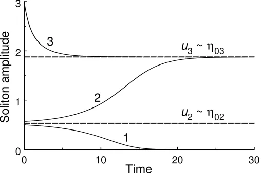
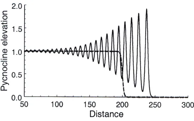
[image:13.612.142.466.325.527.2]

Transient processes. The single pulse solution to the KdV equation in the form of Eq. (22) is very simple, and readily provides physical insight when examined. However, a common observation in the ocean is of wave-trains consisting of several oscillations with wavelengths, crest lengths, and amplitudes varying from the front to the rear of the wavetrain (as schemat-ically shown in Fig. 1 plotted from a simple theoretical model of evolution of an initial step-function within the framework of the KdV equation). As these oscillations, especially the few frontal ones, are very close to being a series of solitons (indeed, each oscillation develops into independent soliton at inﬁnity), and the entire perturbation represents an undular bore, it is sometimes called solibore (Apel, 2003).

Figure 1: Disintegration of a stepwise perturbation into a train of solitons within the frame-work of the KdV equation (a simplistic scheme of solibore formation). Axes are in arbitrary units.

Korteweg and de Vries(1895) had already found periodic solutions to their equation

in the form of the so-called “cnoidal” waves, which involve the Jacobi elliptic function cns(x).

This function has a nonlinear parameter, s, that characterizes the degree of non-linearity, with 0≤s≤1. For the KdV equation, the cnoidal solution is given by [see, e.g. (Karpman, 1973)]:

6_{This parameter is known in nonlinear wave theory as the similarity parameter of the KdV equation} (Karpman, 1973). In this paper we use the term “Ursell parameter” from the surface-wave terminology

(14)

η(x, t) = ηm+η0cn2s[k0(x−V t)] (29)

In the above solutionη₀ is the wave magnitude,ηm is the constant background and k0 is

the wavenumber; the soliton velocityV can be expressed in terms of these parameters. This solution reduces to a harmonic wave whens → 0 and cnsx →cosx, and to a solitary wave

whens→1 and cnsx→sech2x. Thus, the soliton can be considered as a limit of a periodic

wave train at s= 1.

However, there is still some ocean phenomenology missing from the cnoidal solution. Speciﬁcally, it does not describe transient processes such as the onset and the long-term trailing edge displacement of the isopycnal surfaces behind the wave group. Using an ap-proximate approach suggested byWhitham(1974),Gurevich & Pitaevskii (1973)have

constructed a self-similar solution for the evolution of an initially stepwise perturbation into a train of oscillations with a slow variation of the nonlinear parameter s within the train. In the process of evolution, these oscillations become deep at the front of the perturbation forming a set of separated impulses, each close to a soliton, and eventually decrease to a constant trailing edge. A recent review on further development of the Gurevich & Pitaevskii approach can be found in El et al., 2005. An exact analytical solution describing the

disintegration of a stepwise initial perturbation into solitons was obtained by Khruslov

(1975, 1976) using an inverse scattering method. Figure 1 illustrates such a process.

To describe an oceanic nonlinear wave train with oscillatory behavior at the leading edge and a constant depression at the trailing edge, Apel(2003) has applied the Gurevich

& Pitaevskii approach to modeling the internal solibores. For a stepwise initial impulse exerted on a ﬂuid att= 0, the solution of the KdV equation is given by:

η(x, t) = ηm+η0

dn2_s[k₀(x−V t)]−(1−s2), (30) where dns(x) is another periodic elliptic function (Jacobi delta-amplitude) which tends to

unity at s→0 and to sech2(x) whens →1; ands is a slowly varying function of xand t. This solution, which Apel has named the “dnoidal” wave, can be suitable for describing weakly nonlinear internal tides. For this case, initial tidal perturbations have a ﬁnite duration and are relatively smooth. Thus, the process of solibore formation includes a stage of wave steepening and the subsequent formation of oscillations. The ﬁrst stage may be described by the equation of a “simple wave” which is in fact a KdV equation with β = 0, i.e. the dispersionless KdV equation. Each point of such a wave propagates at its own velocity,

c+αη, until the wave front becomes steep [see the details in (Apel, 2003; El et al., 2005)]. At that point, the dispersion eﬀects must be taken into account, which leads to the

formation of solitons at the frontal zone of each tidal period, which smoothly transfer to a dnoidal wave with variable parameters at the rear. To accommodate this relaxation back to the equilibrium state, Apel introduced an “internal tide recovery function”I(x, t), which multiplies the dnoidal solution. This function takes the dnoidal solution back to equilibrium, using just one adjustable parameter which is the time required for the relaxation to occur.

3.3.2 The Extended and Modiﬁed Korteweg–de Vries Equations

(15)

close to the middle of the water layer. In this case the nonlinear coeﬃcientαis small or even equal to zero. As mentioned before, in this case one must either abandon the Boussinesq and rigid lid approximations or take into account higher-order nonlinear terms in the evolution equations. In the latter case, the extended Korteweg–de Vries (eKdV) equation (also called the combined KdV and Gardner equation), having both quadratic and cubic nonlinearities, results (Lee & Beardsley, 1974; Djordjevic & Redekopp, 1978; Kakutani & Yamasaki, 1978; Miles, 1979; Gear & Grimshaw, 1983; Smyth & Holloway,

1988; Lamb & Yan, 1966):

∂η ∂t +

c+αη+α₁η2∂η ∂x +β

∂3η

∂x3 = 0, (31)

where for the case of two-layer ﬂuid the second nonlinear coeﬃcient is

α₁ = 3c

h2₁h2₂

⎡ ⎣7

8

ρ₂h2₁−ρ₁h2₂ ρ₂h₁+ρ₁h₂

₂

− ρ2h31+ρ1h32

ρ₂h₁+ρ₁h₂

⎤ ⎦_{≈ −}3

8c

(h₁+h₂)2+ 4h₁h₂

h2₁h2₂ . (32)

The last expression is again valid for the case of close densities which we shall consider below. This equation, as well as its generalization containing a combination of higher-order nonlinear and dispersive terms, was derived by many authors starting from the paper by Lee & Beardsley (1974). A contemporary derivation, convenient for applications, can be found, e.g. in (Djordjevic & Redekopp, 1978; Grimshaw et al., 2002b).

As follows from Eq. (32), within the framework of two-layer model,α₁ is always negative. However, in the general case the coeﬃcientα₁ may be either negative or positive (Grimshaw et al., 1997; Talipova et al., 1999).

If the pycnocline is located just at the critical level so that the parameter α is exactly zero, Eq. (31) reduces to the well-known modiﬁed Korteweg–de Vries (mKdV) equation. In the geophysically most interesting case, when α₁ < 0 and β > 0, this equation has no stationary solitary wave solutions asymptotically vanishing at x → ±∞. However, it has a particular solution that is a type of stepwise transition, which can be considered to be a soliton in a more general sense. Such a solution is usually called a kink and has the form of a bore moving into a depression area (Perelman et al., 1974; Ono, 1976; Romanova, 1979; Miles, 1981; Grosse, 1984; Funakoshi & Oikawa,1986):

η=±η₀tanh

x−vt

∆

, (33)

where now

V =c+α1η

2 0

3 , and ∆

2 ₌₋ 6β

α₁η2₀. (34)

Note that the vertical velocity component w ∂η/∂t has the form of a localized pulse, so that it may properly be treated as a soliton. The speciﬁc feature of such a kink is that its velocity,V, is always less then the linear velocity, c, due to α₁ <0.

Internal bores in a two-layer ﬂuid were recently considered in ( Dias & Vanden-Broeck, 2003). They studied numerically the structure of steady-state bores of arbitrary

(16)

reaches either the upper or lower boundary (i.e. free surface or bottom). Limiting depres-sion bores always have monotonic fronts, whereas their counterparts in elevation may have non-monotonic proﬁles.

The hydrodynamic stability of internal solitons and bores has been only scarcely studied. However, waves in a two-layer ﬂuid always create a discontinuity of the tangential velocity at a pycnocline. In particular, for a bore such a velocity jump extends far behind its front. In general, in such a shear ﬂow, the Kelvin–Helmholtz instability does exist (e.g. Stepanyants & Fabrikant, 1996). This issue is interesting because some observations of internal bores

in lakes, seas, and oceans have already been reported (see, e.g. Thorpe, 1971; Winant,

1974;Ivanov & Konyaev, 1976).

The mKdV equation also has soliton-type solutions, but only those propagating on a constant nonzero pedestal (Perelman et al., 1974; Ono, 1976; Romanova, 1979; Fu-nakoshi & Oikawa, 1986). These solutions are interesting not so much by themselves

as they are within the framework of the eKdV Eq. (31) with α = 0 (note that under the transformationη =u−α/2α₁, Eq. (31) can be reduced to the mKdV form). In this case the solitary solution of Eq. (31) can be written in the form of a kink-antikink pair of a stationary shape:

η(x, t) = −α

α₁ ν

2

tanh

_x₋_{V t}

∆ +φ

−tanh

_x₋_{V t}

∆ −φ

, (35)

or, equivalently,

η(x, t) = −α

α₁ ν

2

sinh(2φ)

cosh2[(x−V t)/∆] + sinh2φ, (36)

where ν is a free dimensionless parameter with the range 0 < ν < 1, and the remaining parameters are

φ(ν) = 1 4ln

_{1 +}_ν

1−ν

, ∆ =

−24α₁β

α2ν2 , V =c− α2ν2

6α₁ . (37)

In contrast with the kink described by (33) and (34), the velocity of this soliton is always greater than the linear velocityc. This family of solutions has rather interesting properties. The amplitude of the soliton, η₀ = −(α/α₁)νtanhφ, varies from zero up to a maximum of

|α/α₁|, in contrast to the amplitude of the KdV soliton, which in principle can range from zero to inﬁnity. When soliton amplitude approaches its maximum value, its width increases so that the soliton proﬁle changes from the bell shape to the rectangular shape. In the limit

ν→1, the eKdV soliton tends to two inﬁnitely separated kinks.

In the near-critical situation when h₁ ≈h₂ =h and the eKdV equation is indeed appli-cable, the amplitude does not exceed|h₂ −h₁|/2, and the velocity cannot exceed the value of

Vmax =c−

α2

6α₁ c

1 + (h2−h1)

2

8h2

. (38)

(17)

[image:17.612.179.432.158.312.2]

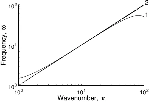
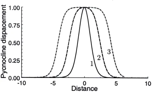
characterized by the parameter S = φ(ν)∆. In general, the actual width of the soliton is determined by these parameters, which in turn depend on the hydrodynamic environment and the amplitude through the free parameter ν. Figure 2 shows normalized shapes of solitons for three values of the modiﬁed free parameter ≡ 1−ν. The evolution from a classical KdV soliton when ν is small and the characteristic total width D ≈ 2∆ to the ﬂat-top kink–antikink construction at ν→1 , in which case D≈2S, is clear.

Figure 2: Normalized wave shapes in the eKdV equation (35) for three values of the param-eter ε= 1−ν: 1 – ε= 10−1 (close to the KdV case); 2 – ε= 10−4; 3 – ε= 10−7.

The width of the soliton increases in both limits: ν → 0 and ν → 1. Hence, for some

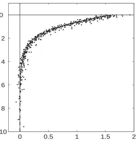
ν=νmthere exists a minimum value ofD. Figure 3 depictsD0.5, the full width of the soliton

at the half its maximum amplitude, as a function of the amplitude, η₀. The minimum of

D₀.5 occurs atν≈0.9, when the amplitude is about 0.56 of the maximum. A more detailed

[image:17.612.168.439.517.683.2]

discussion of the dependency between D and η₀ both for weakly nonlinear perturbations, described by the eKdV equation, and for more intensive perturbations, described by the primitive Eulerian equations, can be found in the paper byFunakoshi & Oikawa(1986).

Figure 3: Dependency of the characteristic width, D₀.5, of eKdV solitons, Eq. (35), on

(18)

From Eq. (37) it follows that

η₀ =−αν

α₁

√

1 +ν−√1−ν

√

1 +ν+√1 +ν (39)

withν related to φ and ∆ by Eqs. (37).

An interesting observation was made in (Grimshaw et al., 1997) and (Talipova et al., 1999). It has been shown that given a certain hydrology (density stratiﬁcation), the

cubic nonlinear coefficient α₁ may in fact become positive. In particular, this is the case of a three-layer fluid with two density jumps located symmetrically with respect to the middle of the fluid layer. The coefficients of the eKdV equation (31) for one of two internal modes in the Boussinesq approximation (ρ₁ ≈ρ₂) are

c=

∆ρ

ρ gh, α= 0, α1 =−

3c

4h2

13− 9H 2h

, β = ch 4 H−

4h

3

, (40)

where H is the total ﬂuid depth and h < H/2 is the thickness of the upper and the lower layers. At the critical thickness,hcr = 9H/26, both quadratic and cubic nonlinear coeﬃcients

vanish (however for another mode, the coeﬃcientα remains nonzero). Apparently, the next order nonlinearity must be taken into account in this case.

Higher-order KdV equations containing corrections both to the nonlinear and dispersive terms have been derived for internal waves in a stratiﬁed shear ﬂows in many papers be-ginning from the aforementioned pioneering paper by Lee & Beardsley (1974). For a

rather general and convenient form of this derivation, see, e.g. (Grimshaw et al., 2002b)

and (Poloukhina et al, 2002). In the case of positive cubic nonlinearity (e.g., when

h < 9H/26, where H is the total ﬂuid depth), solitons of both positive and negative po-larities may exist on a zero background. In addition to that, nonstationary solitons, called breathers, are also possible. The evolution of initial pulse-type perturbation may be fairly complex (Grimshaw et al., 1997).

The mathematical theory of the eKdV equation has been developed in many papers for diﬀerent combinations of signs of nonlinear and dispersion terms (Miles, 1981; Marchant & Smith, 1996; Slyunyaev & Pelinovskii, 1999; Slyunyaev, 2001; Grimshaw et

al., 2002a). It was shown that the eKdV equation and its reduced version, the mKdV

equa-tion, are also completely integrable equations as is the usual KdV equation. In particular,

Slyunyaev & Pelinovskii(1999) have studied in detail the evolution of an initial pulsed

disturbance and analyzed an exact two-soliton interaction in the case when the dispersion and cubic nonlinear coeﬃcients of Eq. (31) are of opposite signs (i.e. β > 0 and α₁ < 0).

Gorshkov & Soustova(2001) suggested an approximate description of the multi-soliton

interaction based on the perturbation theory for solitons and kinks. This theory was applied to an experimental situation in the ocean (Gorshkov et al., 2004).

The evolution of initial perturbations in the case when the dispersion and cubic nonlinear coeﬃcients of Eq. (31) are of the same signs (β >0 and α₁ >0) was studied inSlunyaev, 2001. And Grimshaw et al. (2005) have shown that this situation is typical for the shelf

zones of the World Ocean.

(19)

Michallet & Barth´elemy, 1998). The reason for this is a qualitative (but in general not

quantitative!) correspondence of the eKdV solitons to those of strongly nonlinear solitary waves in a two-layer ﬂuid. The correspondence relates, in particular, to the non-monotonic dependence of their width on the amplitude and to the existence of a limiting amplitude.

3.3.3 The Benjamin–Ono Equation

An important modiﬁcation is needed if the wavelength is large compared with one (say, upper) layer but small compared with the other (lower) layer of the ocean, so that one can let h₂ → ∞. These waves can be described by another completely integrable model, namely by by the diﬀerential-integral Benjamin–Ono (BO) equation [see, e.g. ( Ablowitz & Segur, 1981)]:

∂η ∂t +c

∂η ∂x +αη

∂η ∂x +

β π

∂2 ∂x2℘

∞

−∞

η(x, t)

x−x dx

_{= 0}_, ₍₄₁₎

where the symbol ℘ indicates that the principal value of the integral should be taken, and the coeﬃcients are

c=

(ρ₂−ρ₁)gh₁

ρ₁ , α =−

3 2

c

h₁, β = ch₁

2

ρ₂

ρ₁. (42)

Solitons described by this equation are also well known:

η(x, t) = η0

1 + (x−V t)2/∆2. (43) Their amplitudesη₀, velocities V, and half-widths ∆ are related by

V =c+αη0

4 , and ∆ = 4β

αη₀. (44)

The displacement of these solitons is a downgoing motion of the interface when the upper layer is thin, and conversely for the case when the thin layer lies near the bottom (there is a general thumb rule: pycnocline displacement induced by a soliton is directed to the deepest layer).

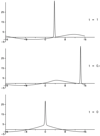
As in most integrable cases, the BO solitons restore their parameters after a collision. However, unlike the KdV case, the displacement in the BO soliton decreases algebraically, as

x2, rather than exponentially (therefore they are often called “algebraic solitons”). Another diﬀerence is that BO solitons do not acquire a phase shift after a collision. As was shown by D. Pelinovsky & C. Sulem in 1998, they are stable with respect to small perturbations and can emerge from arbitrary pulse-type initial perturbations of appropriate polarity, i.e., the polarity required for the existence of a BO soliton.

3.3.4 The Joseph–Kubota–Ko–Dobbs (JKKD) Equation

Apparently, Whitham (1974) was the ﬁrst to point out explicitly that a linear evolution

(20)

a hydrodynamic nonlinearity of the type η_∂x∂η. This approach, albeit not quite consistent, leads to useful model equations in cases when the regular derivation is cumbersome or even impossible.

Following these ideas, Joseph (1977) and Kubota et al. (1978) introduced a model

evolution equation, which is termed here the JKKD equation7. It describes weakly nonlinear perturbations propagating within a thin oceanic layer surrounded from above and below by thick homogeneous layers of fluid of arbitrary depth. A similar equation was later derived rigorously by Segur & Hammack (1982) for a slightly different configuration in which a

layer of lighter ﬂuid overlies a layer of heavier ﬂuid. The thickness of one of the layers, say the upper one,h₁, is assumed to be small in comparison with the thickness of a lower layer,

h₂, i.e. h₁/h₂ 1. At the same time the perturbation wavelength, λ h₁, may have an arbitrary relationship withh₂, i.e. the total water layer can be either shallow or deep. The resulting evolution equation can be presented in a variety of equivalent forms; one of the simplest is

∂η ∂t +c

∂η ∂x +αη

∂η ∂x −β

∂2 ∂x2℘

∞

−∞

η(x/h₂, t)

tanhπ₂x−_hx

2

dx = 0, (45)

where, for the two-layer model with a sharp density interface, the parameters c and α are the same as in Eq. (41) andβ =ch₁/(4h₂).

The dispersion relation corresponding to this equation and relating the wavenumber k

with a frequency ω of the linear perturbations, η∼exp (kx−ωt), is

ω =ck 1− kh1 2 tanhkh₂

. (46)

In the shallow-water (kh₂ → 0) and deep-water (kh₂ → ∞) limits this reduces to the KdV and BO dispersion relations, respectively.

The JKKD equation has a solitary solution which has been obtained by many authors and presented in diﬀerent forms (Joseph, 1977; Chen & Lee, 1979; Segur & Hammack, 1982). One of the forms convenient for practical applications is

η(x, t) = η0

1 + 2

1 + cos2h2

∆

sinh2x−V t ∆

, (47)

where

η₀ = 4 3

h2₁

∆

sin2h2

∆

1 + cos2h2

∆

, V =c 1− h1 ∆ tan2h2

∆

. (48)

Here ∆ is a free parameter characterizing the soliton width.

Equations (47) and (48) reduce to a KdV soliton, Eqs. (22) and (23), in the limit of

h₂/∆→0, for a ﬁxedh₁/h₂. Meanwhile, as was pointed out by Chen & Lee (1979), there

is no smooth transition from the JKKD soliton to the BO soliton as h₂ → ∞, in contrast with Joseph’s claim (Joseph, 1977). This issue still remains unclear because Eq. (45) tends

to either the KdV or the BO limit ash₂ →0 or h₂ → ∞, respectively. Chen & Lee(1979)

also found a periodic solution for the JKKD equation, which reduces to the algebraic BO

(21)

soliton of the form of Eq. (43) but only for one ﬁxed set of parametersη₀, V,and ∆. Segur & Hammack (1982) have derived the next-order correction to the wave amplitude for the

JKKD equation, and have obtained the corresponding corrections to the JKKD soliton. The main features of the initial perturbation dynamics within the framework of the JKKD equation are very similar to those described by the KdV model. It is worth noting here that all the models considered above, beginning from the KdV, are analytically integrable, pos-sessing an inﬁnite set of conservation laws and multi-soliton solutions [see, e.g. (Ablowitz & Segur, 1981)]. Their properties have been thoroughly studied by mathematicians.

However seemingly crude it may be, the two-layer model often gives a good approximation to situations in which the density and velocity vary continuously but sharply with depth; this occurs especially for the ﬁrst vertical mode in near-shore regions where moderate depths are the rule. This may be seen, for example, in a comparison between the two-layer model and a more exact model based on a smooth density proﬁle (Ivanov et al., 1992) which

was measured in the Levant Sea (the eastern Mediterranean). The validity of the two-layer models and their comparison with results from laboratory experiments are discussed in the afore-mentioned report byOstrovsky & Stepanyants(2005). An optimal adjustment of

the two-layer model parameters which gives the best approximation for wave velocities and other observable wave characteristics in the real ocean is discussed in (Nagovitsyn et al., 1990) and (Gerkema, 1994). However, in other cases the parameters of the corresponding

equations must be calculated from the expressions (21), (16) corresponding to a general case of a continuously stratiﬁed ﬂuid (see, e.g. (Ostrovsky & Stepanyants, 1989), and

references therein).

From an observational viewpoint, it is important to remember that a single measurement of a solitary-like formation does not guarantee that the entity is indeed a soliton. An initial impulse may quickly disintegrate afterwards into something other than a solitary wave. In principle, it is necessary to follow such a wave out to a distance much greater than its spatial width to ensure that its shape remains stationary, which is not a simple task in real experiments. Another criterion for identiﬁcation of a soliton is based on knowledge of the background density and horizontal velocity proﬁles. After a theoretical calculation of soliton parameters, one can compare these with the observational data. For example, the product of the characteristic wave width ∆ and the square root of its height, √η₀, must not depend on that height [cf. Eq. (23)], provided the KdV equation is applicable to the situation considered.

3.4

Soliton Propagation Under Perturbations.

(22)

“time-like” KdV (TKdV) equation8 (in the context of internal waves see, for example, Liu et al., 1985):

∂η ∂r + 1 c ∂η ∂t − αη c2 ∂η ∂t − β c4

∂3η ∂t3 =−

η

2r − η

2c dc

dr +R(η). (49)

The terms in the right-hand side of Eq. (49) describe, respectively, the eﬀects of cylin-drical divergence (the distance r from the source is supposed to be much greater than the wavelength), slow variation of the long-wave speedcalong the ray r due to spatial inhomo-geneity (e.g. due to variation of the pycnocline depth), and dissipation.

The latter term depends on a speciﬁc mechanism of losses. In particular, a horizontal eddy (turbulent) viscosity A_[h] and a molecular viscosity νm result in dissipation that is

described by a Reynolds-type term, R = _cδ₂∂_∂t2₂η (δ is proportional to the sum of A_[h] and

νm, and usually A[h] νm). Semi-empirical models accounting for bottom friction are

also used, resulting in the terms R = γRaη (Rayleigh dissipation) and R = γCh|η|η (Chezy

dissipation) withγRa,γCh taken as empirical coeﬃcients (Holloway et al., 1997, 1999, 2002; Grimshaw, 2002). A rigorous consideration of viscous eﬀects in the laminar bottom

boundary layer leads to inclusion into Eq. (49) of a more complex integral term (Grimshaw, 1981, 2002; Das & Chakrabarti, 1986).

From Eq. (49), an ordinary diﬀerential equation for the slow variation of the soliton amplitudeη₀ over large distances can be obtained. As follows from perturbation theory [see, e.g. (Ostrovsky, 1974)], the ﬁrst-order solution of Eq. (49) for the soliton amplitude may

be obtained by multiplying it byη, substituting the soliton (22), (23) with locally constant parameters, and then integrating over inﬁnite limits in time,−∞< t <∞. One obtains

dη₀ dr =−

2η₀

3r −

2η₀

3c dc dr −

4αδ

45βη

2

0, (50)

which describes slow variations of the soliton amplitude under the eﬀect of small cylindrical divergence, horizontal inhomogeneity, and eddy and molecular viscosity. The variations of length and width of the soliton are then deﬁned via the local relation, Eq. (23), as before.

As particular cases, we readily obtain the laws of soliton variability due to (a) cylindrical divergence (δ = 0, c= const):

η₀ ∼ r−2/3, ∆ ∼ r1/3. (51) These dependencies were examined in the laboratory experiments with surface and in-ternal waves (Weidman & Zakhem, 1988) and very good agreement between the theory

and experiment was obtained;

(b) a smooth horizontal variation of cin a plane wave:

η₀ ∼ c−2/3. (52)

According to Eq. (23), variations of ∆ are not directly deﬁned byc(or η₀) but rather by a combination of the parametersβ and α, which may change together with c.

(c) the separate eﬀect of Reynolds losses results in the following damping law:

8_{This term has been introduced by} Osborne (1995) for the version of KdV equation with transposed

(23)

η₀(r) = η0(0)

1 +η₀(0)qr, (53)

where η₀(0) is the initial soliton amplitude, and q = 4αδ/β. From Eq. (53) it is seen that soliton damping is non-exponential because of the nonlinearity. Moreover, at large dis-tances, r [η₀(0)q]−1, the soliton amplitude ceases to depend on its initial value at all9,

η₀(r) ∼ (qr)−1. Chezy friction leads to the same law of soliton attenuation (Grimshaw, 2002; Caputo & Stepanyants, 2003), whereas Rayleigh dissipation yields an

exponen-tial damping with an exponent diﬀerent from that for linear waves (Ostrovsky, 1983; Caputo & Stepanyants, 2003).

Soliton decay due to energy dissipation in the laminar boundary layer is described by an integral dissipative term [see, e.g., Grimshaw, 2002; Ostrovsky & Stepanyants, 2005and references therein]:

R(η) =−δ₁

+∞

−∞

1−sgn(t−t)

|t−t|

∂η(t, x)

∂t dt

_. ₍₅₄₎

The dissipation coeﬃcient δ₁ depends, in general, on many parameters such as the depth, density, and viscosity of the ﬂuid layers (Leone et al., 1982). However, in the Boussinesq

approximation with the additional assumption that kinematic viscosities of layers are also equal,ν₁ =ν₂ ≡νm, this coeﬃcient may be presented in a relatively simple form (Helfrich, 1992)10:

δ₁ = 1 4c

νm/π

h₁+h₂

b+ (1 +b)

2

2b + 2 h₂

W(1 +b)

, (55)

whereb=h₁/h₂ and W is the width of the tank. The applicability of this dissipation model requires the boundary-layer thickness to be much less than the total water depth.

For such dissipation, the following damping law for soliton amplitude follows from the adiabatic theory:

η₀(r) = η0(0) (1 +r/rch)4

, (56)

whererchis the characteristic spatial scale of soliton decay (see details in the references cited

above). Forrrch this formula gives η0(r)∼r−4, and the soliton amplitude also ceases to

depend on its initial value [becauserch ∼η−1 /4 0 (0)].

The perturbed KdV and eKdV equations similar to Eq. (49) were used in numerical modeling of the internal tide transformation on the Australian north-west shelf, the Malin shelf edge (western cost of Scotland), and the Arctic shelf (Laptev Sea) (Holloway et al., 1997; 1999; 2002; Grimshaw et al., 2005). The spatial variability of the coeﬃcients,

the Earth’ rotation and bottom friction eﬀects were taken into account in those papers. We should remark also that in case (a), Eq. (49) represents the cylindrical KdV equation, which is completely integrable. This equation possesses exact solitary solutions (Calogero & Degasperis, 1978; Nakamura & Chen, 1981), whose parameters vary in space due

9_{A similar behavior is known in nonlinear acoustics for weak shock waves having a sawtooth form.} 10_{A misprint in the numerator of formula (A6) of} Helfrich’s_{paper of 1992 should be mentioned, it must}

(24)

to cylindrical divergence, in agreement with equation (51) as obtained by the asymptotic method. Note ﬁnally that to describe soliton transformation, diﬀerent models may have to be employed sequentially. For example, a cylindrically diverging soliton in the BO model decreases as 1/r; after its broadening due to amplitude decrease, it can eventually be trans-formed into a cylindrical KdV soliton behaving according to Eq. (51) (Stepanyants, 1981).

An interesting kind of dissipation of interfacial internal waves can occur in the deep ocean when a sharp pycnolcine is adjoined by a smoothly stratiﬁed layer of “inﬁnite” depth (depth much greater than the thickness of the other layer and the characteristic wavelength). In this case, the governing model equation for the interface perturbation is similar to the JKKD equation but contains a more complex integral kernel, which describes both the dispersion and the dissipation due to the radiation of downward propagating bulk internal waves (Maslowe & Redekopp, 1980; Grimshaw, 1981) [see also (Grimshaw, 2002)].

According to estimates from these papers made for typical oceanic conditions, such solitary waves may decay in a time comparable to their intrinsic time scale,Tint ∼∆/V.

3.5

Refraction and Diﬀraction of Solitons

Various generalizations of the KdV equation have been suggested for nonlinear waves having smoothly curved phase fronts. One of the most popular is the Kadomtsev–Petviashvili (KP) equation, which is applicable to a weakly diﬀracted wave beam, and is based again on adding a small term to the KdV equation describing transverse variations:

∂ ∂x

∂η ∂t +c

∂η ∂x +αη

∂η ∂x +β

∂3η ∂x3

=−c 2

∂2η

∂y2, (57)

where y is the coordinate transverse to the propagation direction x. This equation is also known to be completely integrable. Its exact solutions have been studied in numerous papers and books (see, e.g. Ablowitz & Segur, 1981; Infeld & Rowlands, 1990).

The main properties of solitary solutions to this equation as applied to oceanic waves (when the dispersion parameter is always positive,β > 0) are as follows. A plane soliton is stable with respect to transverse perturbations of its front. Multiple soliton interactions can occur when solitons propagate in diﬀerent directions at small angles to each other. The zone of nonlinear interaction of two solitons can be fairly long in space; the perturbation in this zone looks like a KdV soliton and propagates steadily. The interaction between two solitons has been studied in detail byNewell & Redekopp(1977) and Miles(1977a, b). They found

a speciﬁc case of resonant interaction of two obliquely propagating solitons where the the zone of nonlinear interaction is inﬁnite and forms another stationary soliton

For waves propagating at small angles to an arbitrarily chosen direction in the horizontal plane, the 2D analogs of the BO and JKKD equations may also be derived (Ablowitz & Segur, 1981). These equations, however, are apparently not integrable. The transverse

stability of a BO soliton was studied and conﬁrmed byAblowitz & Segur (1981).

Two-soliton interaction was studied numerically by Tsuji & Oikawa (2001). They found that

the phenomenon similar to the resonant interaction of KP solitons does occur for the BO equation, too. However, the concept of resonant interaction is not so eﬀective for that equation, because the newly generated wave in the zone of nonlinear interaction of two solitons is far from the BO soliton.

(25)

expressed via each other [see (Stepanyants, 1989) and references therein].

Another approach to studying two-dimensional eﬀects is the “nonlinear geometrical op-tics” of solitons, which describes refraction of their fronts. The theory is based on the method elaborated earlier by Whitham (1974) for shock waves and then extended to solitons by Ostrovsky & Shrira(1976). It considers the motion of soliton fronts in orthogonal

co-ordinates (Φ,Ψ) corresponding to lines of constant phase and normals to them, or “rays,” at succeeding moments of time. This leads to a pair of kinematic equations:

V ∂θ ∂Ψ =

∂R ∂Φ,

(58)

R∂θ

∂Φ = −

∂V ∂Ψ,

where R is the dimensionless width of the ray tubes, and θ is the angle between the rays and some reference direction. In the case considered, this system must be closed by using a dynamic relation reﬂecting the conservation of soliton energy; in particular, for the KdV equation it is

R(V −c)2∆(V) = const, (59) where ∆ is the soliton width. From this, the system of Eqs. (58) may be shown to possess two characteristics that deﬁne the propagation speed during perturbations of the soliton amplitude and the shape of the wave front. These perturbations, being strong, propagate as simple (Riemann) waves with the possible formation of “shocks,” i.e. sharp jumps in amplitude and frontal direction. As also occurs in the dynamics of compressible gases, one needs a form of dissipation or a “viscosity” to smooth out this shock. As shown byShrira

(1980), weak radiation of small amplitude waves from the soliton front in the process of soliton adjustment to the local hydrological conditions may play the role of such a viscosity in