Topology optimization of geometrically nonlinear structures using an evolutionary optimization method

Full Terms & Conditions of access and use can be found at

http://www.tandfonline.com/action/journalInformation?journalCode=geno20

Engineering Optimization

ISSN: 0305-215X (Print) 1029-0273 (Online) Journal homepage: http://www.tandfonline.com/loi/geno20

Topology optimization of geometrically nonlinear

structures using an evolutionary optimization

method

Meisam Abdi, Ian Ashcroft & Ricky Wildman

To cite this article: Meisam Abdi, Ian Ashcroft & Ricky Wildman (2018): Topology optimization of geometrically nonlinear structures using an evolutionary optimization method, Engineering Optimization, DOI: 10.1080/0305215X.2017.1418864

To link to this article: https://doi.org/10.1080/0305215X.2017.1418864

© 2018 The Author(s). Published by Informa UK Limited, trading as Taylor & Francis Group

Published online: 19 Jan 2018.

Submit your article to this journal

Article views: 29

View related articles

https://doi.org/10.1080/0305215X.2017.1418864

Topology optimization of geometrically nonlinear structures

using an evolutionary optimization method

Meisam Abdi a,b, Ian Ashcroft aand Ricky Wildman a

a_{Faculty of Engineering, University of Nottingham, Nottingham, UK;}b_{Faculty of Technology, De Montfort University,} Leicester, UK

ABSTRACT

The topology optimization using isolines/isosurfaces and extended finite element method (Iso-XFEM) is an evolutionary optimization method devel-oped in previous studies to enable the generation of high-resolution topology optimized designs suitable for additive manufacture. Conven-tional approaches for topology optimization require addiConven-tional post-processing after optimization to generate a manufacturable topology with clearly defined smooth boundaries. Iso-XFEM aims to eliminate this time-consuming post-processing stage by defining the boundaries using isoval-ues of a structural performance criterion and an extended finite element method (XFEM) scheme. In this article, the Iso-XFEM method is further developed to enable the topology optimization of geometrically nonlinear structures undergoing large deformations. This is achieved by implement-ing a total Lagrangian finite element formulation and definimplement-ing a structural performance criterion appropriate for the objective function of the opti-mization problem. The Iso-XFEM solutions for geometrically nonlinear test cases implementing linear and nonlinear modelling are compared, and the suitability of nonlinear modelling for the topology optimization of geometrically nonlinear structures is investigated.

ARTICLE HISTORY Received 25 October 2016 Accepted 22 November 2017

KEYWORDS Topology optimization; XFEM; geometrically nonlinear; evolutionary; mesh refinement

1. Introduction

There has been significant interest in topology optimization methods and applications over the past three decades, stemming from the groundbreaking article of Bendsøe and Kikuchi (1988), which introduced the homogenization method. Other methods developed after this include solid isotropic material with penalization (SIMP) (Bendsøe1989; Zhou and Rozvany1991), evolutionary structural optimization (ESO) (Xie and Steven1993; Xie and Steven1997), bidirectional evolutionary structural optimization (BESO) (Querin, Steven, and Xie1998; Yanget al.1999; Aremuet al.2013), level-set method (Wang, Wang, and Guo2003; Allaire, Jouve, and Toader2004) and evolutionary-based algo-rithms,e.g.the genetic algorithm (GA) (Jakielaet al.2000) and differential evolution (DE) (Fioreet al.

2016). Although many of the proposed topology optimization algorithms have been demonstrated for classical problems, such as Michell-type structures and cantilever beams with rectangular domains, less attention has been paid to applying these algorithms to three-dimensional (3D), real-life struc-tures and real loading scenarios. In some cases, the mathematical complexity or the size of the finite element (FE) design domain does not allow the algorithm to be properly implemented. OptiStruct

CONTACT Meisam Abdi [email protected]

© 2018 The Author(s). Published by Informa UK Limited, trading as Taylor & Francis Group

(Altair Engineering) is an example of software designed to enable the SIMP method of topology optimization to be applied to real components. Other software such as Nastran (MSC Software) and Abaqus FEA (Dassault Systèmes) also have options to apply similar density-based approaches to find the solution to topology optimization problems. Although the topology optimization modules of these software applications are widely used for research and engineering purposes, a drawback of the density-based approaches (and many other element-based approaches) is that they cannot provide a clear and smooth representation of the design boundaries in converged topologies. This issue brings difficulties in interpreting the solutions, combining them with computed-aided design and manufac-turing the topologies. Therefore, the solutions usually need post-processing, reanalysing and shape optimization before manufacturing.

Previous attempts to improve the surface quality of optimized solutions include the use of remesh-ing/adaptive mesh techniques with topology optimization. Aremuet al. (2011) presented a hybrid algorithm for topology optimization consisting of a modified form of the BESO method and an adap-tive meshing strategy. A level-set-based r-refinement method was proposed by Yamasaki, Yamanaka, and Fujita (2017) to generate a conforming mesh during the topology optimization process. The use of hierarchical remeshing strategies for the BESO method was investigated by Panesaret al. (2017). Nana, Cuillière, and Francois (2016) employed h-refinement to improve definition of the solid–void interface of SIMP solutions. Wang, Kang, and He (2013,2014) proposed an adaptive mesh refinement strategy based on independent point-wise density interpolation for topology optimization. The idea was to refine the displacement field and the density field separately, aiming to achieve solutions with high quality at a reasonable computational cost. As an alternative to adaptive topology optimization, the topology optimization using isolines/isosurfaces and extended finite element method (Iso-XFEM) was developed in a previous study to address the issues related to the boundary representation of the topology (Abdi, Wildman, and Ashcroft2014; Abdi, Ashcroft, and Wildman2014,2014). The idea was to use a simple evolutionary-based optimization algorithm (similar to BESO) while improving the boundary representation by implementing an isoline/isosurface approach during the optimiza-tion. An extended finite element method (XFEM) integration scheme was also used to increase the accuracy of FE solutions near the design boundary. The method was successfully applied to two-dimensional (2D) and 3D structures with complex design domains (Abdi, Ashcroft, and Wildman

2014), and the results showed a significant improvement in boundary representation and structural performance of the solutions over conventional BESO.

The majority of work regarding topology optimization of structures is based on linear modelling of the problems, assuming that the structure contains only linear elastic materials and undergoes small displacements. Although this assumption can be effectively applied to a large range of structural design problems, there are still many cases that require nonlinear modelling to obtain valid solutions. Large deformation is a significant source of nonlinearity that can be found in many nonlinear prob-lems. Examples of such problems include energy absorption structures and compliant mechanisms, which can be classified generally as ‘geometrically nonlinear structures’.

considered topology optimization of nonlinear compliant mechanisms represented with frame ele-ments. Bruns and Tortorelli (2003) proposed an element removal and reintroduction strategy for topology optimization problems with geometric nonlinearity. Ha and Cho (2008) and Luo and Tong (2008) developed a level-set-based topology optimization method for large-deformation problems. Huang and Xie (2007,2008) applied BESO for topology optimization of geometrically nonlinear structures under both force loading and displacement loading.

An important consideration when applying topology optimization techniques to nonlinear struc-tures should be the computational efficiency of the method, as the analysis requires much more computation than that of a linear structure. This becomes even more important when applying the method to 3D structures. The other issue that may arise in density-based topology optimization approaches such as SIMP is the existence of intermediate densities in the solutions. Because of the large displacements, the tangent stiffness matrix of low-density elements may become indefinite or even negatively definite during the optimization process (Buhl, Pedersen, and Sigmund2000; Bruns and Tortorelli2003). To overcome this issue, Bruns and Tortorelli (2003) proposed totally remov-ing low-density elements. To stabilize the excessive distortion of low-density elements, Lahuertaet al. (2013) proposed the use of a polyconvex constitutive model in conjunction with a relaxation function. Wanget al. (2014) proposed a new interpolation scheme in which the strain energy density (SED) of low-density elements and high-density elements was modelled using small deformation theory and large deformation theory, respectively. An element deformation scaling approach was used by van Dijk, Langelaar, and van Keulen (2014) to scale the local internal displacements in low-density ele-ments. Huang and Xie (2007,2008) suggested using hard-kill BESO to increase the computational efficiency and avoid issues regarding the existence of intermediate-density elements.

The application of the Iso-XFEM method to the topology optimization of geometrically non-linear structures could be of significant benefit because of its high computational efficiency and lack of intermediate-density elements in the solutions, while it still benefits from high-resolution boundary representation. In the next sections of this article, after presenting an overview of the Iso-XFEM method, a nonlinear modelling strategy for geometrically nonlinear structures based on an incremental–iterative Newton–Raphson approach is presented. An appropriate structural perfor-mance criterion for stiffness design is derived and the Iso-XFEM method is demonstrated for several large-deformation problems.

2. Overview of the Iso-XFEM method

The main three elements of the Iso-XFEM method are an isoline/isosurface approach to represent the design boundary, XFEM to calculate the elemental sensitivities (a structural performance crite-rion) near the boundary, and an evolutionary-based optimization algorithm. These three elements are explained in this section.

2.1. Isoline/isosurface approach

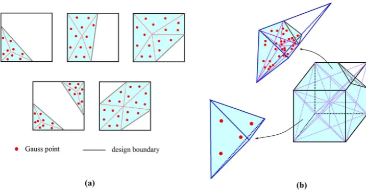
Isolines/isosurfaces are the lines/surfaces that represent the points at which a function has a con-stant value, named the isovalue, in a 2D/3D space. In structural optimization applications (Abdi, Wildman, and Ashcroft2014; Abdi, Ashcroft, and Wildman2014; Victoria, Martí, and Querin2009; Victoria, Querin, and Martí2010), the boundaries are defined by the intersection of the structural per-formance (SP) distribution with a minimum level of perper-formance (MLP), which typically increases during the optimization process. Figure1(a) shows a 2D fixed grid design domain discretized with a 30×30 mesh, where the intersection of SED distribution as a structural performance criterion with a minimum level of SED gives the design boundary. The relative performance,α, is defined as

Figure 1.(a) Boundary representation using isolines of a structural performance (SP) function [strain energy density (SED)]. The intersection of SP distribution with the minimum level of performance (MLP) defines the current state of the boundary. (b) Implicit representation of a two-dimensional design space and the structure’s geometry using relative structural performance (α). (c) Design space decomposed into the solid region (_{α(x) >}0), void region (_{α(x) <}0) and boundary (_α(x)=0).

The design domain can be partitioned into the void phase, boundary and solid phase, with respect to the values of relative performance:

α(x):

⎧ ⎪ ⎨ ⎪ ⎩

>0 solid phase (DS)

=0 boundary (∂DS) <0 void phase (DV)

(2)

Figure1(b) and (c) shows how the design space,D, from Figure1(a) is partitioned intoDS,∂DS

andDVusing the relative performance functionα(x), distributed over the design space.

2.2. XFEM

(Sukumaret al.2001)

u(x)=

i

Ni(x)H(x)ui (3)

whereNi(x) are the classical shape functions associated with the nodal degrees of freedom,ui. The

value of the Heaviside functionH(x) is equal to 1 for the nodes and regions in the solid part of the design and switches to 0 for nodes and regions in the void part of the design domain. Based on the above displacement function, the stiffness matrix of an element with material–void discontinuity is given by (Sukumaret al.2001)

ke= ∫

B

T_{CH(x)Bd (4)}

whereis the element domain,Bis the displacement differentiation matrix, andCis the elasticity matrix for the solid material. This XFEM scheme was realized by dividing the solid domain of the boundary elements into sub-triangles (in 2D problems as shown in Figure2(a)) or sub-tetrahedra (in 3D problems as shown in Figure2(b)), and then performing numerical integration over solid triangles/tetrahedra using the Gauss quadrature method (Abdi, Ashcroft, and Wildman2014).

The XFEM decomposition scheme shown in Figure2requires finding the solid domain of bound-ary elements before decomposing it into triangles/tetrahedra. The solid domain of a boundbound-ary element can be defined using solid nodes of the element (nodes with positive values of relative per-formance) and the intersection points of the element edges and the boundary,i.e.points with zero value of relative performance which can be found through bilinear (in 2D) or trilinear (in 3D) inter-polation of relative performance (α) between the nodes. Various decomposition schemes can then be employed to define sub-triangles/sub-tetrahedra for numerical integration, resulting in a similar numerical accuracy (Li, Wang, and Wei2012). For instance, the solid region of quadrilateral elements in Figure2(a) was decomposed into sub-triangles by connecting a central point of the solid region to the surrounding solid nodes and intersection points. Similarly, a hexahedral element can be initially decomposed to a number of tetrahedra. For those tetrahedra that lie on the boundary, the solid region of the tetrahedra can be further decomposed into sub-tetrahedra (Figure2(b)), with the numerical integration being performed over all solid tetrahedra.

2.3. Evolutionary-based optimization method

The optimization algorithm used in the Iso-XFEM method is evolutionary based,i.e.based on the simple assumption that the optimized solution can be achieved by gradually removing the inefficient material from the design domain. However, unlike ESO, in which the material removal is carried out at an elemental level, in this approach the optimization operates at a global level of structural performance by the use of an isoline/isosurface design approach. An appropriate performance cri-terion is used to characterize the efficiency of material usage in the design domain. Material is then removed from low relative performance regions (x;α(x)<0) and redistributed to the high relative performance regions (x;α(x)>0). The target volume of the design for the current iteration needs to be calculated before any region is added to or removed from the structure. The target volume of the design for the current iteration is given by

Vit =max(Vit−1(1−ER),Vc) (5)

whereERis the volume evolution rate andVcis the specified volume constraint. Once the target vol-ume of the current iteration is found, the minimum level of performance that gives this volvol-ume needs to be identified. This could be achieved through an iterative process, for instance by defining upper and lower bands for MLP (which are equal to the maximum and minimum structural performance in the first iteration, respectively), finding the volumes corresponding to the upper and lower bands, averaging and updating the upper and lower bands until the difference between the volumes corre-sponding to the upper and lower bands is smaller than a minimum value. The evolutionary process continues until the volume fraction condition is satisfied. From this time forwards, the optimiza-tion process runs with a constant volume fracoptimiza-tion (as given by Equaoptimiza-tion 5) until the changes in the objective function in the last five iterations are within a specified tolerance.

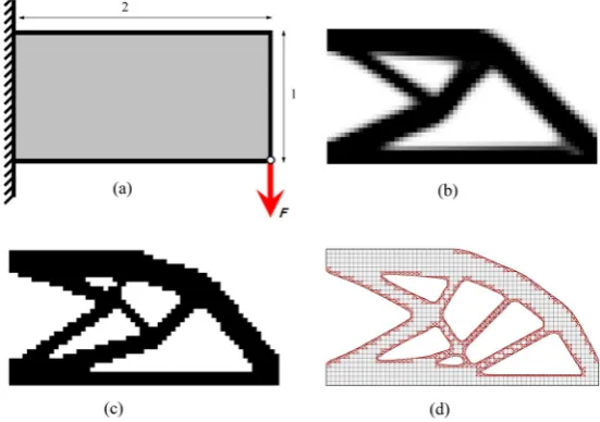
Figure3compares solutions achieved using SIMP, BESO and Iso-XFEM for the cantilever problem of Figure3(a) assuming linear deformations. It can be seen that the Iso-XFEM solution (Figure3(d)) is represented with clearly defined boundaries, unlike the SIMP (Figure3(b)) and BESO (Figure3(c)) solutions, in which the solutions are represented with variable element densities and/or back-ground mesh-defined boundaries. A more in-depth comparison of the methods in terms of solution

Figure 4.Illustration of the incremental Newton–Raphson approach.

performance can be found in Abdi, Wildman, and Ashcroft (2014) and Abdi, Ashcroft, and Wildman (2014).

3. Modelling geometric nonlinearity

3.1. Incremental–iterative approach

In this study, the incremental Newton–Raphson approach is utilized to find the equilibrium solu-tion at every evolusolu-tionary iterasolu-tion. In this approach, the applied load (R) is first divided into a set of smaller load increments. Then, starting from the first load increment, using the tangent stiffness matrix (KT), the displacement caused by that force increment is computed. Using the accumulated

displacement, the resistant force (F) is obtained and the unbalanced force (tR−tF), which is the dif-ference between the applied and the resistant forces, is determined. The iterative process at this load increment continues by calculating a new tangent stiffness matrix, finding the displacement and the unbalanced force (Figure4). The equations used in the Newton–Raphson method can be stated as (Bathe2006)

t+t_K

T(it−1)u(it)=t+tR−t+tF(it−1)

t+t_u(it)₌t+t_u(it−1)_+u(it) ₍₆₎

where t is a suitably chosen time increment andit denotes the iteration number of the New-ton–Raphson procedure in each time increment. The initial conditions at the start of each time increment are:

t+t_u(0)₌t_u; t+t_K(0)

T =tKT; t+tF(0) =tF (7)

Convergence is achieved when both the errors, measured as the Euclidean norms of the unbalanced forces and of the residual displacements, are less than a minimum value. The complete equilibrium path can be traced by finding the subsequent solution points at higher load levels using the same approach.

3.2. Geometrically nonlinear behaviour of a continuum body

a new measure for stress, the second Piola–Kirchhoff stress tensor, has to be introduced with the Green–Lagrange strain tensor. Considering TL formulation for a general body subjected to applied body forcesfBand surface tractionsfSon the surface S and displacement fieldδui, the equation of

motion is given by (Gea and Luo2001)

0_V

Sijδijd0V =

0_V

f_iBδuid0V+

0_S

f

f_iSδuiSd0S (8)

whereSijdenote the Cartesian components of the second Piola–Kirchhoff stress tensor,δijare the

components of the Green–Lagrange strain tensor corresponding to the virtual displacement fieldδui,

and0V denotes the body volume at initial configuration. The Green–Lagrange strain tensor, which is defined with respect to the initial configuration of the body, is given by (Gea and Luo2001)

ij= 1

2

_∂

ui ∂0_x

j + ∂uj ∂0_x

i + ∂uk ∂0_x

i ∂uk ∂0_x

j

(9)

Considering reasonably small strains, the general elastic constitutive equation can still be used:

Sij=Cijklij (10)

whereCis the elasticity tensor. Equations (8)–(10) are the basic equations for calculating the response of a continuum body using the TL formulation. However, to solve these equations for strongly non-linear problems, one may need to use an incremental–iterative approach, such as Newton–Raphson, as discussed in Section3.1.

3.3. Continuous form of the equilibrium equation

Introducing the incremental approach to find the structural responses in nonlinear structures, one can decompose the displacements, strains and stresses at timet+tas

t+t_u

i=tui+ui; t+tij=tij+ij; t+tSij=tSij+Sij (11)

whereui,ijandSijdenote the displacements, strains and stresses increments, respectively, to

be determined. The strain increments can be defined as the sum of linear and nonlinear terms as

ij=eij+ηij (12)

where the linear incremental strain,eijis given by

eij= 1

2

_∂

ui ∂0_x

j + ∂uj

∂0_x

i + ∂uk

∂0_x

j ∂t_u

k ∂0_x

i + ∂uk

∂0_x

i ∂t_u

k ∂0_x

j

(13)

and the nonlinear incremental strain,ηijis defined by

ηij= 1

2

∂uk ∂0_xi

∂uk

∂0_xj (14)

Implementing Equation (11) into the equilibrium equation (Equation 8) and assumingSij=

Cijkleijandδij=δeij, the linearized incremental equation of motion is obtained as

0_V

cijkleijδekld0V+

0_V t_S

ijδηijd0V=

0_V t+t_fB

i δuid0V+

0_Sf t+t_fS

iδuSid0S−

0_V t_S

ijδeijd0V (15)

3.4. Finite element formulation

Transforming the continuous form of the equation of motion represented by Equation (15) to an FE formulation, the equilibrium equation is obtained as (Gea and Luo2001; Bathe2006)

t_K

TU=(K0+Kd+Kσ)U=F (16)

wheretKTis the tangent stiffness matrix andFis the load imbalance between the external forces t+t_{Rand the internal forces}t_F.K

0is the usual small displacement stiffness matrix represented by

K0=

V0

BT_L0CBL0d0V (17)

whereBL0 is a linear strain–displacement transformation matrix used in linear infinitesimal strain analysis. The stiffness matrixKdin Equation (16) represents the large displacement stiffness matrix

and is defined by

Kd=

V0

(BT_L0CBL1+BTL1CBL0+BTL1CBL1)d0V (18)

whereBL1is a linear strain–displacement transformation matrix which depends on the displacement.

Kσin Equation (16) is the initial stress matrix dependent on the stress level, and is given by

K_σ =

V0

BT_NLtSBNLd0V (19)

where BT_NL denotes the nonlinear strain–displacement transformation matrix and tSdenotes the second Piola–Kirchhoff stress matrix, which in a 2D formulation is defined by

t_S= ⎡ ⎢ ⎢ ⎣ t_S 11 t_S 21 0 0 t_S 12 t_S 22 0 0 0 0 t_S 11 t_S 21 0 0 t_S 12 t_S 22 ⎤ ⎥ ⎥ ⎦ (20)

The correct calculation of the internal forces,tF in Equation (16), is crucial as any error in this calculation will result in an inaccurate response prediction. The internal forces can be found from

t_{F= ∫} V0

(BL0+BL1)T tSd¯ 0V (21)

wheretS¯is the second Piola–Kirchhoff stress vector. Equation (16) is used to find the displacement increment corresponding to the statet+t, which is then added to the displacement at statetto obtain displacement at statet+t. The strain–displacement relation in Equation (9) allows the strain to be determined from the displacements and, using the constitutive relation in Equation (10), one can then calculate the corresponding stresses.

3.5. XFEM for geometrically nonlinear behaviour

21) should be merely performed on the solid region of a boundary element. If four-node quadrilateral elements are used in the FE model of the structure, this can be done by dividing the solid part of the boundary elements into sub-triangles and performing Gauss quadrature (Abdi, Ashcroft, and Wildman2014). Following that, the element’s tangent stiffness matrixtkTcan be obtained from

t_k T=

n

i=1

m

j=1

Aitwjf1(ξ1j,ξ

j

2,ξ

j

3) (22)

whereiandjare the indices regarding the partitions and Gauss points, respectively;nis the number of solid partitions (sub-triangles) inside the element andmis the number of Gauss points in each partition.ξ1:3are the natural coordinates of the Gauss points,Aiis the area of the trianglei,tis the

thickness of the 2D element,wis a weighting factor and

f1=BTCB+BLT0CBL1+BTL1CBL0+BTL1CBL1+BTNLtSBNL. (23)

Internal force vectortFecan be obtained from

t_F e=

n

i=1

m

j=1

Aitwjf2(ξ1j,ξ

j

2,ξ

j

3) (24)

where

f2 =(BL0+BL1)T tS¯ (25) The elements’ tangent stiffness matrices and internal force vectors can then be assembled to obtain the global tangent stiffness matrixtKTand global internal force vectortFof the structure.

4. Stiffness design

4.1. Objective function and structural performance criteria

To find the stiffest design, the natural choice is to minimize the deflection or compliance. However, the drawback of this objective function is that it may result in structures that can only support the maximum load for which they are designed and may break down for lower loads (Buhl, Pedersen, and Sigmund2000). To avoid this, when the nonlinear structure is loaded under force control, the com-plementary workWCcan be chosen as the objective function (Figure5). In this case, the optimization problem can be defined as:

Minimize :f(x)=WC= lim

n→∞

1 2

n i=1

RT(Ui−Ui−1)

subject to :

n e=1v

s e=Vc

(26)

whereRis the load increment,idenotes the increment number, andnis the total number of load increments.

The sensitivity of the objective functions with respect to design variablexeis:

Se= ∂f(x) ∂xe =

lim n→∞ 1 2 n

i=1

(RT_i −RT_i−1)

_∂

Ui ∂xe −

∂Ui−1

∂xe

(27)

Figure 5.Objective function_WCfor stiffness optimization of nonlinear structures under force control.

Solving the above equation, the elemental sensitivity numbers for nonlinear structures under force control are obtained as the total elemental elastic and plastic strain energy,Ene(Huang and Xie2010).

This can be used in BESO as the criterion for element removal and addition to find the solution for stiffness optimization of nonlinear structures. Similarly, in the Iso-XFEM optimization method, the elemental sensitivity numbers can be used to find the structural performance:

SPe= E n e

Ve

(28)

4.2. Filter scheme for Iso-XFEM

To increase the stability of the Iso-XFEM method applied to geometrically nonlinear problems, a sim-ilar filter scheme to the one used for BESO (Huang and Xie2010) and SIMP (Sigmund2001) can be employed. Here, the purpose of the filter is to smooth the structural performance distribution over the design domain by averaging the nodal values of structural performance with those of neighbouring nodes. The modified values of structural performance can then be defined by

SPi= k

j=1wijSPj k

j=1wij

(29)

wherekis the number of nodes inside a domain centred at nodeihaving a filter radius ofrmin, and

wijare the weighting factors defined by

wij=rmin−rij (30)

whererijis the distance between nodeiand the neighbouring nodej.

4.3. Iso-XFEM procedure for geometrically nonlinear structures

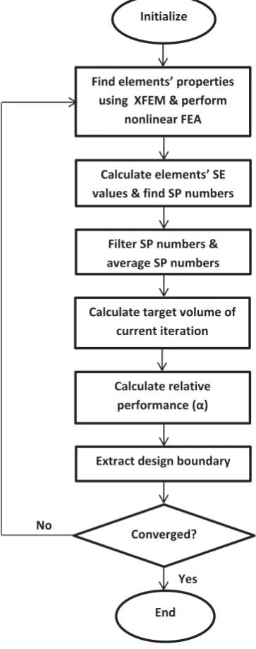
The Iso-XFEM procedure for stiffness design of geometrically nonlinear structures can be summa-rized as the following steps, as also illustrated in Figure6.

• Initialize: define the design space, non-design domain, material properties, a fixed grid FE mesh, loads and boundary conditions, and the optimization parameters.

• Perform nonlinear finite element analysis (FEA): divide the applied load into a suitable number of load increments and find the equilibrium path using the Newton–Raphson approach. Find the properties of the boundary elements using the XFEM scheme.

Figure 6.Flowchart of the extended finite element method using isolines/isosurfaces (Iso-XFEM) for geometrically nonlinear struc-tures. XFEM₌extended finite element method; FEA₌finite element analysis; SE₌strain energy; SP₌structural performance.

• Filter structural performance numbers.

• Average the structural performance numbers with those of the previous iteration.

• Calculate the target volume of the current iteration and find a minimum level of performance to meet the target volume.

• Find the relative performance,α, over the design domain and extract the design boundary. Assign solid material properties to regions havingα >0 and void material properties to the regions havingα <0.

5. Examples

5.1. Test case 1: nonlinear cantilever plate

The cantilever plate shown in Figure7was considered as the first test case of this study. This beam has been used as a test case in previous studies, implementing SIMP (Buhl, Pedersen, and Sigmund2000) and BESO (Huang and Xie2010), allowing comparison of the Iso-XFEM solutions with the other two methods. The cantilever plate was 1 m in length, 0.25 m in width and 0.1 m in thickness, and was subjected to a concentrated load at the middle of the free end. The material used was nylon, which has a Young’s modulus ofE=3 GPa and Poisson’s ratio ofv=0.4. Nonlinear, stiffness-optimized designs of the plate with a volume constraint of 50% of the design domain under two point loads 60 kN and 144 kN were investigated and compared. A mesh of 200×50 quadrilateral elements was used for the FE model of the structure. A relatively low evolution rate ofER=0.005 was used to increase the stability of the nonlinear Iso-XFEM method by performing the material removal within a higher number of evolutionary iterations,i.e.applying less change to the topology at each iter-ation. A filter radius ofrmin=1.2 times the element size was used. The reason for using a small filter radius was to stabilize the evolutionary process without significantly changing the complexity of the solutions.

Figure8shows the evolution histories of the objective function (WC) and volume fraction for both load cases, 60 kN and 144 kN. It can be seen that the evolutionary optimization process of the nonlinear structure subjected to the point load of 60 kN (Figure8(a)) has good stability. However, by increasing the load to 144 kN (Figure8(b)),i.e.increasing the degree of nonlinearity, some insta-bility was observed in the plot of complementary work (iteration 70 afterwards). Figure9shows the solutions obtained from the linear and nonlinear optimization for the two different load val-ues. Note that linear Iso-XFEM solutions for both load cases are the same when the same target volume fraction is used. It can be seen that the linear Iso-XFEM has converged to a symmetrical solution. This is expected as the design is optimized with respect to the equilibrium geometry of the undeformed beam. However, different designs are obtained by implementing the nonlinear topology design, showing that the optimal topologies depend on the magnitude of the applied load. These are now non-symmetrical as the design is optimized for the deformed beam under load, which is not symmetrical. The large deformation of the Iso-XFEM solutions is illustrated in Figure10. Table1

compares the objective values (complementary works) of the linear and nonlinear Iso-XFEM solu-tions with those previously investigated using SIMP (Buhl, Pedersen, and Sigmund2000) and BESO (Huang and Xie2010), implementing the same objective function. It can be seen that the nonlinear designs obtained from both Iso-XFEM designs have lower magnitudes of complementary work than their linear designs, indicating a better performance for the load for which they are designed. Also comparing the Iso-XFEM with BESO and SIMP solutions in terms of their complementary work, it can be seen that the Iso-XFEM solutions have lower magnitudes of complementary work than the BESO and SIMP solutions, showing better performance of the Iso-XFEM solutions owing to their smooth boundary representation. The slightly higher complementary work of the SIMP solutions compared to the BESO solutions was attributed to the effect of intermediate-density elements in SIMP

Figure 8.Evolution histories of the objective function and volume fraction of the nonlinear cantilever subjected to a point load of (a) 60 kN, and (b) 144 kN.

Table 1.Comparison of the complementary works of linear and nonlinear designs for test case 1.

Complementary work Design forF=60 kN Design forF=140 kN

Linear design from Iso-XFEM 2.107 kJ 12.072 kJ

Nonlinear design from Iso-XFEM 2.101 kJ 12.063 kJ

Nonlinear design from BESO (Huang and Xie2010) 2.171 kJ 12.38 kJ

Nonlinear design from SIMP (Buhl, Pedersen, and Sigmund2000) 2.331 kJ 13.29 kJ

Note: Iso-XFEM=topology optimization using isolines/isosurfaces and extended finite element method; BESO=bidirectional evolutionary structural optimization; SIMP₌solid isotropic material with penalization.

solutions, where their strain energy may have been overestimated (Huang and Xie2010). This can-tilever problem has also been studied for compliance minimization (Buhl, Pedersen, and Sigmund

2000; He, Kang, and Wang2014). In this case, a different solution with a tail member was reported. However, as pointed out by Buhl, Pedersen, and Sigmund (2000) and Huang and Xie (2010), the solu-tions achieved from minimizing compliance may not support a load lower than the maximum load for which they are designed.

The test case presented in this section shows that by using nonlinear FE modelling in the Iso-XFEM method, a different solution with a higher performance than the linear design can be achieved. However, it could be argued that the difference in the overall topology of the linear and nonlinear solutions of this test case was insufficient to justify the extra effort of the nonlinear analysis. As will be shown in the next example, in some cases the difference can be extremely large and can make the use of nonlinear modelling essential.

5.2. Test case 2: slender beam

Figure 9.Extended finite element method using isolines/isosurfaces (Iso-XFEM) solutions of the large-displacement cantilever problem: (a) linear design (for both load cases of 60 kN and 144 kN); (b) nonlinear design for a point load of 60 kN; (c) nonlinear design for a point load of 144 kN.

Figure 10.Illustration of the large deformation of the cantilever plate: (a) cantilever subjected to a point load of 60 kN; (b) cantilever subjected to a point load of 144 kN. The deformations are to scale.

structure. In this type of problem, radically different topologies can be obtained using linear and nonlinear modelling in the structural optimization problem. As an example of a structure involv-ing snap-through effects, the topology optimization of a slender beam with the design domain and boundary conditions shown in Figure11was considered. The beam was 8 m long, 1 m deep and 100 cm thick. A load of 400 kN was applied to the centre of the top edge The material properties of the beam were a Young’s modulus ofE=3 GPa and Poisson’s ratio ofv=0.4. Nonlinear and lin-ear stiffness-optimized designs of the beam for a volume constraint of 20% of the design domain for downward and upward loads were investigated. A mesh of 320×40 quadrilateral elements was used for the FE model of the structure in all the experiments, and a volume evolution rate ofER =0.01 and a filter radius ofrmin=1.2 times the element size were used as optimization parameters.

Figure 11.Design domain and boundary conditions of the geometrically nonlinear slender beam of test case 2: (a) beam subjected to downward load; (b) beam subjected to upward load.

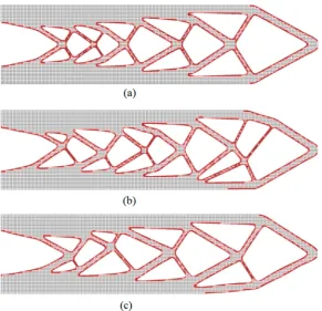
Figure 12.(a) Nonlinear design of the beam subjected to a downward load; (b) nonlinear design of the beam subjected to an upward load; (c) linear design of the beam (for both downward load and upward load cases).

Figure 13.(a) Displacement of solution shown in Figure12(a); (b) displacement of solution shown in Figure12(b); (c) displacement of solution shown in Figure12(c) subjected to downward load; (d) displacement of solution shown in Figure12(c) subjected to upward load. The deformations are to scale.

Table 2.Comparison of the complementary works of nonlinear and linear designs for test case 2.

Complementary work Design for downward load Design for upward load

Nonlinear design from Iso-XFEM 38.700 kJ 36.492 kJ

Linear design from Iso-XFEM 55.548 kJ 36.494 kJ

Note: Iso-XFEM=topology optimization using isolines/isosurfaces and extended finite element method.

is not an issue when linear modelling is used, with nonlinear modelling the thin compressed beams buckle and the whole structure experiences snap-through, as seen in Figure13(c). The snap-through effect was not an issue for the upward loading as the thin struts were not put under compression, hence the similarity of the linear and nonlinear designs for upward loading (Figure13(b) and (d)). Table2

compares the complementary works of the solutions subjected to downward and upward loads. As anticipated, the difference between the complementary works of nonlinear and linear solutions for the upward load case is not significant. However, in the case of the downward load case, the comple-mentary work of the linear design involving buckling and snap-through effects is much higher than for the nonlinear one, showing the importance of implementing a nonlinear topology optimization approach for large-displacement problems such as those involving snap-through effects.

5.3. Further remarks on the efficiency of the proposed method

The test cases studied in this article showed how the Iso-XFEM method can benefit from nonlin-ear modelling, especially when the method is applied to problems with a high degree of geometric nonlinearity. However, it should be noted that the computational cost of optimization significantly increases when nonlinear modelling is used. For example, in test case 1, the time cost of the opti-mization with linear modelling was 3020 s for 100 iterations. Using the same desktop computer for the analysis, the corresponding time cost for optimization of the cantilever under 140 kN load with nonlinear modelling was 15,895 s for 100 iterations. The increased computational cost of nonlinear modelling can become problematic when applying the method to 3D problems with a high num-ber of FEs. However, compared to conventional element-based methods of topology optimization, an advantage of the Iso-XFEM method is that it requires fewer elements to return a high-resolution solution, thus saving on the computational cost of the optimization (Abdi, Wildman, and Ashcroft

2014; Abdi, Ashcroft, and Wildman2014).

The formulation adopted in this article was based on the assumption that the structure undergoes large deformation with small strains. However, if the strains are large or if the material behaviour is nonlinear, different formulations will be required for the nonlinear modelling. The test cases studied in this article (cantilever beam and slender beam) are frequently used benchmark problems within the topology optimization community, allowing the comparison of Iso-XFEM solutions with the solutions from previously developed methods such as SIMP and BESO. Moreover, cantilever and slender beam members exist in many engineering applications, from microscale parts,e.g.atomic force microscope cantilevers and micro-electromechanical system cantilevers/beams, to large struc-tures,e.g.bridges and civil structures. The application of the method to real problems may require the definition of alternative objective functions and the derivation of appropriate sensitivities. Examples are the design of compliant mechanisms, where the objective can be to maximize the output defor-mation, and the design of energy absorption structures, where the objective may be to maximize the total absorbed energy.

6. Summary and conclusions

nonlinear behaviour of continuum structures and a Newton–Raphson iterative method was used to find the equilibrium solution at each load increment. The nonlinear FE code developed for 2D struc-tures was then integrated into the Iso-XFEM method to enable the topology optimization of strucstruc-tures undergoing large deformation. A filter scheme was used in the method to increase the stability of the evolutionary optimization approach applied to nonlinear structures.

The topology optimization results achieved by implementing linear and nonlinear modelling showed that, for the presented test cases, a nonlinear-based optimization returns solutions that are dependent on the magnitude of the load. In addition, the solutions achieved from the optimization using nonlinear modelling have a higher performance than those with linear modelling. Although in the first test case of this study, there is not a significant difference between the solutions achieved from linear and nonlinear modelling, the results from the second test case, which involves snap-through effects, showed the importance of implementing nonlinear modelling in large-displacement prob-lems. As the solutions achieved from the proposed method are represented with clearly defined and smooth boundaries, the time-consuming post-processing stage before manufacturing can be elimi-nated. This makes the method suitable for the stiffness design of digitally manufactured structures,

e.g.3D printed structures, which experience large deformation.

Disclosure statement

No potential conflict of interest was reported by the authors.

Funding

This work was supported by the Engineering and Physical Sciences Research Council [grant number EP/I033335/2].

ORCID

Meisam Abdi http://orcid.org/0000-0003-2320-7509

Ian Ashcroft http://orcid.org/0000-0002-5118-1804

Ricky Wildman http://orcid.org/0000-0003-2329-8471

References

Abdi, M., I. Ashcroft, and R. Wildman.2014. “An X-FEM Based Approach for Topology Optimization of Continuum Structures.” InSimulation and Modeling Methodologies, Technologies and Applications, 277–289. Cham: Springer International Publishing.

Abdi, M., I. Ashcroft, and R. Wildman.2014. “High Resolution Topology Design with Iso-XFEM.” InProceedings of

the 25th Solid Freeform Fabrication Symposium (SFF2014), 1288–1303.https://sffsymposium.engr.utexas.edu/sites/

default/files/2014-101-Abdi.pdf

Abdi, M., R. Wildman, and I. Ashcroft.2014. “Evolutionary Topology Optimization Using the Extended Finite Element Method and Isolines.”Engineering Optimization46 (5): 628–647.

Allaire, G., F. Jouve, and A. M. Toader.2004. “Structural Optimization Using Sensitivity Analysis and a Level-Set Method.”Journal of Computational Physics194 (1): 363–393.

Aremu, A., I. Ashcroft, R. Wildman, R. Hague, C. Tuck, and D. Brackett.2011. “A Hybrid Algorithm for Topology

Opti-mization of Additive Manufactured Structures.” InProceedings of the 22nd Solid Freeform Fabrication Symposium

(SFF2011), 279–289.https://sffsymposium.engr.utexas.edu/Manuscripts/2011/2011-22-Aremu.pdf

Aremu, A., I. Ashcroft, R. Wildman, R. Hague, C. Tuck, and D. Brackett.2013. “The Effects of Bidirectional Evolutionary Structural Optimization Parameters on an Industrial Designed Component for Additive Manufacture.”Proceedings

of the Institution of Mechanical Engineers, Part B: Journal of Engineering Manufacture227 (6): 794–807.

Bathe, K. J.2006.Finite Element Procedures. Englewood Cliffs, NJ: Prentice Hall.

Bendsøe, M. P.1989. “Optimal Shape Design as a Material Distribution Problem.”Structural Optimization1: 193–202. Bendsøe, M. P., and N. Kikuchi.1988. “Generating Optimal Topologies in Structural Design Using a Homogenization

Method.”Computer Methods in Applied Mechanics and Engineering71: 197–224.

Bruns, T. E., and D. A. Tortorelli.1998. “Topology Optimization of Geometrically Nonlinear Structures and Compliant Mechanisms.” InProceedings of the 7th AIAA/USAF/NASA/ISSMO Symposium on Multidisciplinary Analysis and

Bruns, T. E., and D. A. Tortorelli.2003. “An Element Removal and Reintroduction Strategy for the Topology Optimiza-tion of Structures and Compliant Mechanisms.”International Journal for Numerical Methods in Engineering57 (10): 1413–1430.

Buhl, T., C. B. Pedersen, and O. Sigmund.2000. “Stiffness Design of Geometrically Nonlinear Structures Using Topology Optimization.”Structural and Multidisciplinary Optimization19 (2): 93–104.

Fiore, A., G. C. Marano, R. Greco, and E. Mastromarino.2016. “Structural Optimization of Hollow-Section Steel Trusses by Differential Evolution Algorithm.”International Journal of Steel Structures16 (2): 411–423.

Gea, H. C., and J. Luo.2001. “Topology Optimization of Structures with Geometrical Nonlinearities.”Computers &

Structures79 (20): 1977–1985.

Ha, S. H., and S. Cho.2008. “Level Set Based Topological Shape Optimization of Geometrically Nonlinear Structures Using Unstructured Mesh.”Computers & Structures86 (13): 1447–1455.

He, Q., Z. Kang, and Y. Wang.2014. “A Topology Optimization Method for Geometrically Nonlinear Structures with Meshless Analysis and Independent Density Field Interpolation.”Computational Mechanics54 (3): 629–644. Huang, X. H., and Y. Xie.2007. “Bidirectional Evolutionary Topology Optimization for Structures with Geometrical

and Material Nonlinearities.”AIAA Journal45 (1): 308–313.

Huang, X., and Y. M. Xie.2008. “Topology Optimization of Nonlinear Structures Under Displacement Loading.”

Engineering Structures30 (7): 2057–2068.

Huang, X., and M. Xie.2010.Evolutionary Topology Optimization of Continuum Structures: Methods and Applications. Chichester: John Wiley & Sons.

Jakiela, M. J., C. Chapman, J. Duda, A. Adewuya, and K. Saitou.2000. “Continuum Structural Topology Design with Genetic Algorithms.”Computer Methods in Applied Mechanics and Engineering186 (2): 339–356.

Jog, C.1996. “Distributed-Parameter Optimization and Topology Design for Non-linear Thermoelasticity.”Computer

Methods in Applied Mechanics and Engineering132 (1–2): 117–134.

Lahuerta, R. D., E. T. Simões, E. M. Campello, P. M. Pimenta, and E. C. Silva.2013. “Towards the Stabilization of the Low Density Elements in Topology Optimization with Large Deformation.”Computational Mechanics52 (4): 779–797. Li, L., M. Y. Wang, and P. Wei.2012. “XFEM Schemes for Level Set Based Structural Optimization.”Frontiers of

Mechanical Engineering7 (4): 335–356.

Luo, Z., and L. Tong.2008. “A Level Set Method for Shape and Topology Optimization of Large-Displacement Compliant Mechanisms.”International Journal for Numerical Methods in Engineering76 (6): 862–892.

Nana, A., J. C. Cuillière, and V. Francois.2016. “Towards Adaptive Topology Optimization.”Advances in Engineering

Software100: 290–307.

Panesar, A., D. Brackett, I. Ashcroft, R. Wildman, and R. Hague.2017. “Hierarchical Remeshing Strategies with Mesh Mapping for Topology Optimisation.”International Journal for Numerical Methods in Engineering111: 676–700. doi:10.1002/nme.5488.

Pedersen, C. B., T. Buhl, and O. Sigmund.2001. “Topology Synthesis of Large-Displacement Compliant Mechanisms.”

International Journal for Numerical Methods in Engineering50 (12): 2683–2705.

Querin, O. M., G. P. Steven, and Y. M. Xie.1998. “Evolutionary Structural Optimisation (ESO) Using a Bidirectional Algorithm.”Engineering Computations15 (8): 1031–1048.

Sigmund, O.2001. “A 99 Line Topology Optimization Code Written in Matlab.”Structural and Multidisciplinary

Optimization21 (2): 120–127.

Sukumar, N., D. L. Chopp, N. Moës, and T. Belytschko.2001. “Modeling Holes and Inclusions by Level Sets in the Extended Finite-Element Method.”Computer Methods in Applied Mechanics and Engineering190 (46): 6183–6200. van Dijk, N. P., M. Langelaar, and F. van Keulen.2014. “Element Deformation Scaling for Robust Geometrically

Nonlinear Analyses in Topology Optimization.”Structural and Multidisciplinary Optimization50 (4): 537–560. Victoria, M., P. Martí, and O. M. Querin.2009. “Topology Design of Two-Dimensional Continuum Structures Using

Isolines.”Computers & Structures87 (1): 101–109.

Victoria, M., O. M. Querin, and P. Martí.2010. “Topology Design for Multiple Loading Conditions of Continuum Structures Using Isolines and Isosurfaces.”Finite Elements in Analysis and Design46 (3): 229–237.

Wang, Y., Z. Kang, and Q. He.2013. “An Adaptive Refinement Approach for Topology Optimization Based on Separated Density Field Description.”Computers & Structures117: 10–22.

Wang, Y., Z. Kang, and Q. He.2014. “Adaptive Topology Optimization with Independent Error Control for Separated Displacement and Density Fields.”Computers & Structures135: 50–61.

Wang, F., B. S. Lazarov, O. Sigmund, and J. S. Jensen.2014. “Interpolation Scheme for Fictitious Domain Techniques and Topology Optimization of Finite Strain Elastic Problems.”Computer Methods in Applied Mechanics and Engineering 276: 453–472.

Wang, M. Y., X. Wang, and D. Guo.2003. “A Level Set Method for Structural Topology Optimization.”Computer

Methods in Applied Mechanics and Engineering192 (1): 227–246.

Xie, Y. M., and G. P. Steven.1993. “A Simple Evolutionary Procedure for Structural Optimization.”Computers &

Structures49: 885–896.

Yamasaki, S., S. Yamanaka, and K. Fujita.2017. “Three-Dimensional Grayscale-Free Topology Optimization Using a Level-Set Based r-Refinement Method.”International Journal for Numerical Methods in Engineering112: 1402–1438. doi:10.1002/nme.5562.

Yang, X. Y., Y. M. Xie, G. P. Steven, and O. M. Querin.1999. “Bidirectional Evolutionary Method for Stiffness Optimization.”AIAA Journal37 (11): 1483–1488.