BiLog: Spatial Logics for Bigraphs
1Giovanni Conforti
aDamiano Macedonio
bVladimiro Sassone
baUniversity of Dortmund bUniversity of Sussex
Abstract
Bigraphs are emerging as a (meta-)model for concurrent calculi, like CCS, ambients, π -calculus, and Petri nets. They are built orthogonally on two structures: a hierarchical place graph for locations and a link (hyper-)graph for connections. Aiming at describing bigraph-ical structures, we introduce a general framework, BiLog, whose formulae describe arrows in monoidal categories. We then instantiate the framework to bigraphical structures and we obtain a logic that is a natural composition of a place graph logic and a link graph logic. We explore the concepts of separation and sharing in these logics and we prove that they generalise well known spatial logics for trees, graphs and tree contexts. As an application, we show how XML data with links and web services can be modelled by bigraphs and de-scribed by BiLog. The framework can be extended by introducing dynamics in the model and a standard temporal modality in the logic. However, in some cases, temporal modalities can be already expressed in the static framework. To testify this, we show how to encode a minimal spatial logic for CCS in an instance of BiLog.
Key words: Concurrency, Bigraphs, Spatial Logics, Context Logic, Separation, XML
1 Introduction
To describe and reason about structured, distributed, and dynamic resources is one of the main goals of global computing research. Recently, many spatial logics have been studied to fulfill this aim. The term ‘spatial,’ as opposed to ‘temporal,’ refers to the use of modal operators inspecting the structure of the terms in the model, 1 Research partially supported by the projects ‘DisCo: Semantic Foundations of
rather than a temporal behaviour. Spatial logics are usually equipped with a sepa-ration/composition operator that splits a term into two parts, to ‘talk’ about them separately. The notion of separation is interpreted differently in different logics. • In ‘separation’ logics [34], it is used to reason about dynamic update of heap-like
structures, and it is strong as it forces names of resources in separated compo-nents to be disjoint. Consequently, term composition is usually partially defined. • In static spatial logics, for instance for trees [6], graphs [10] and trees with hidden names [11], the separation/composition does not require any constraint on terms, and names are usually shared between separated parts.
• In dynamic spatial logics, too, the separation is intended only for locations in space (e.g. for ambients [13] orπ-calculus [4]).
Context tree logic, introduced in [7], integrates the first approach above with a spatial logic for trees. The result is a logic able to express properties of tree-shaped structures (and contexts) with pointers, and it is used as an assertion language for Hoare-style program specifications in a tree memory model. Essentially, Spatial Logic founds its semantics on model structure.
Bigraphs [25,28] are an emerging model for structures in global computing, that can be instantiated to model several well-known examples, including λ-calculus [31], CCS [32],π-calculus [25], ambients [26] and Petri nets [29]. Bigraphs consist es-sentially of two graphs sharing the same nodes. The first graph, the place graph, is tree structured and expresses a hierarchical relationship on nodes (viz. locality in space and nesting of locations). The second graph, the link graph, is an hyper-graph and expresses a generic “many-to-many” relationship among nodes (e.g. data link, sharing of a channel). The two structures are orthogonal, so links between nodes can cross locality boundaries. Thus, clarify the difference between structural sepa-ration (i.e., sepasepa-ration in the place graph) and name sepasepa-ration (i.e., sepasepa-ration on the link graph).
In this paper we introduce a spatial logic for bigraphs as a natural composition of a place graph logic, for tree contexts, and a link graph logic, for name linkings. The main point is that a resource has a spatial structure as well as a link structure associated to it. Suppose for instance to be describing a tree-shaped distribution of resources in locations. We may use an atomic formula likePC(A) to describe a resource of ‘type’PC (e.g. a personal computer) whose contents satisfy A, and a formula likePCx(A) to describe the same resource at the location x. Note that the lo-cation type is orthogonal to the name. We can then writePC(T)⊗PC(T) to charac-terise terms with two unnamedPCresources whose contents satisfy the tautological formula (i.e., with anything inside). Named locations, as e.g. inPCa(T)⊗PCb(T), can express name separation, i.e., that names a and b are different (because sep-arated by ⊗). Furthermore, link expressions can force name-sharing between re-sources with formulae likePCa(inc ⊗ T)
c
c, which models, e.g. a communication channel. Name c is used as input (in) for the firstPCand as an output (out) for the secondPC. No other name is shared and
c cannot be used elsewhere insidePCs.
A bigraphical structure is, in general, a context with several holes and open links that can be filled by composition. The logic therefore describes contexts for re-sources at no additional cost. We can then express formulae likePCa(T⊗ HD(id1)), that describes a modular computer PC, where id1 represents a ‘plug-able’ hole in the hard discHD. Contextual resources have many important applications. In par-ticular, the contextual nature of bigraphs is useful to characterise their dynamics, but it can also be used as a general mechanism to describe contexts of bigraphical data structures (cf. [19,23]).
As bigraphs are establishing themselves as a truly general (meta)model of global systems, and appear to encompass several existing calculi and models (see for in-stance [25,26,29,32]), our bigraph logic, BiLog, aims at achieving the same gen-erality as a description language: as bigraphs specialise to particular models, we expect BiLog to specialise to powerful logics on these. In this sense, the contribu-tion of this paper is to propose BiLog as a unifying language for the descripcontribu-tion of global resources. We will explore this path in future work, fortified by the embed-ding results for the static spatial logics presented in §5, and the positive preliminary results obtained for semistructured data (cf.§6) and CCS (cf.§7).
The paper is organised as follows: §2 provides a crash course on bigraphs; §3 intro-duces the general framework and model theory of BiLog; §4 shows how to derive some useful connectives, such as a temporal modality and assertions constraining the “type” of terms; §5 instantiates the framework to obtain logics for place, link and bi-graphs; §6 focus on the applications of BiLog to XML data; §7 studies how to deal with dynamic models. An abridged version of this work appears in the con-ference paper [20] and the application to XML was presented in [19]. Here a new embedding result for a dynamic logic based on CCS [5] is added to our main tech-nical result, that is the embedding of the static spatial logics of [6], [10] and [7] by BiLog. In particular, CCS embedding is based on an structural way of expressing the ‘next-step’ modality by composition adjuncts and bigraphical contexts. More-over we show proofs, examples and properties more in detail. Further examples and technical details can be found in [17,27].
2 An informal introduction to Bigraphs
PC R1
R2
1
2
U
PC
1
w z
y x
2
x y
v
[image:4.595.179.413.74.175.2]G
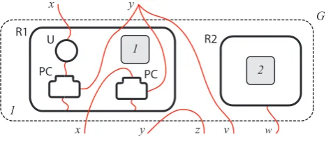
Fig. 1. A bigraph G :h2,{x,y,z,v,w}i → h1,{x,y}i.
ports that may be connected to each other by links, the so-called link graph. Place graphs express locality, that is the physical arrangement of the nodes. Link graphs are hyper-graphs and formalise connections among nodes. The orthogonality of the two structures dictates that nestings impose no constrain upon interconnections. The bigraph G of Fig. 1 represents a system where people and things interact. We imagine two offices with employees logged onPCs. Every entity is represented by a node, shown with bold outlines, and every node is associated with a control (either
PC,U, R1,R2). Controls represent the kinds of nodes, and have fixed arities that determine their number of ports. Control PC marks nodes representing personal computers, and its arity is 3: in clockwise order, the ports represent a keyboard interacting with an employee U, a LAN connection interacting with another PC
and open to the outside network, and the mains plug of the officeR. The employee
Umay communicate with another one via the upper port in the picture. The nesting of nodes (place graph) is shown by the inclusion of nodes into each other; the connections (link graph) are drawn as lines.
At the top level of the nesting structure sit the regions. In Fig. 1 there is one sole region (the dotted box). Inside nodes there may be ‘context’ holes, drawn as shaded boxes, which are uniquely identified by ordinals. The hole marked by 1 represents the possibility for another userUto get into officeR1and sit in front of aPC. The hole marked by 2 represents the possibility to plug a subsystem inside officeR2. Place graphs can be seen as arrows over a symmetric monoidal category whose objects are finite ordinals. We write P : m→ n to indicate a place graph P with m
PC R1 R2 1 2 U PC 1 w z y x 2 x y v G U U PC
x y z v w
1 2
F1 F2
[image:5.595.117.449.75.204.2]PC R1 R2 U PC 1 x y U U PC H
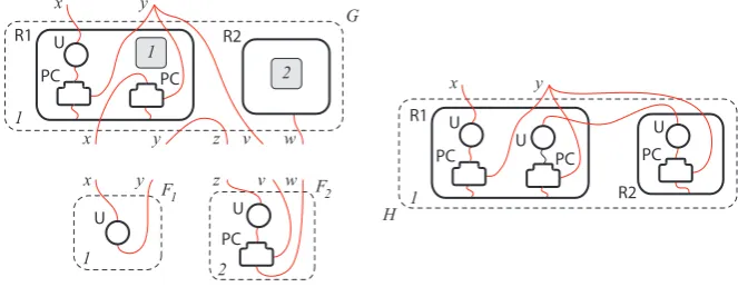
Fig. 2. Bigraphical composition, H ≡G◦(F1⊗ F2).
(drawn on the top). The link graph connects ports to names or to edges (represented in Fig. 1 by a line between nodes), in any finite number. A link to a name is open, i.e., it may be connected to other nodes as an effect of composition. A link to an edge is closed, as it cannot be further connected to ports. Thus, edges are private, or hidden, connections. The composition of link graphs W ◦W0corresponds to linking the inner names of W with the corresponding outer names of W0 and forgetting about their identities. As a consequence, the outer names of W0(resp. inner names of W) are not necessarily inner (resp. outer) names of W ◦ W0. Thus link graphs can perform substitution and renaming, so the outer names in W0 can disappear in the outer names of this means that either names may be renamed or edges may be added to the structure. As in [25], the tensor product of link graphs is defined in the obvious way only if their inner (resp. outer) names are disjoint.
By combining ordinals with names we obtain interfaces, i.e., coupleshm,Xiwhere
m is an ordinal and X is a finite set of names. By combining the notion of place
graph and link graphs on the same nodes we obtain the notion of bigraphs, i.e., arrows G :hm,Xi → hn,Yi.
Figure 2 represents a more complex situation. Its top left-hand side reports the system of Fig. 1, in its bottom left-hand side F1represents a userUready to interact with aPCor with some other users, F2represents a user logged on its laptop, ready to communicate with other users. The system with F1and F2represents the tensor product F = F1 ⊗ F2. The right-hand side of Fig. 2 represents the composition
G ◦F. The idea is to insert F into the context G. The operation is partially defined,
Table 3.1. BiLog terms
G,G0 ::= Ω constructor (for Ω∈Θ)
G◦G0 vertical composition
G⊗G0 horizontal composition
3 BiLog: syntax and semantics
The final aim of the paper is to define a logic able to describe bigraphs and their substructures. Since bigraphs, place graphs, and link graphs are arrows of a (partial) monoidal category, we first introduce a meta-logical framework having monoidal categories as models; then we adapt it to model the orthogonal structures of place and link graphs. Finally, we specialise the logic to model the whole structure of (abstract) bigraphs.
Following the approach of spatial logics, we introduce connectives that reflect the structure of the model. In this case, models are monoidal categories and the logic describes spatially the structure of their arrows.
The meta-logical framework we propose is inspired by the bigraph axiomatisation presented in [30]. The model of the logic is composed by terms of a general lan-guage with horizontal and vertical compositions and a set of unary constructors. Terms are related by a structural congruence that satisfies the axioms of monoidal categories, and possibly more. The corresponding model theory is parameterised on basic constructors and structural congruence. To be as free as possible in choos-ing the level of intensionality, the logic is defined on a transparency predicate. Its role is to identify the terms allowing inspection of their content, transparent terms, and the ones that do not, opaque terms. We inspect the logical equivalence induced by the logic and we observe that it corresponds to the structural congruence when every term is transparent, and it becomes less discriminating with the introduction of opaque terms, cf. §3.2.
3.1 Terms
To evaluate formulae, we consider the terms freely generated from a set of con-structorsΘ, ranged over byΩ, by using the (partial) operators: composition (◦) and tensor (⊗). The order of binding precedence is ◦, ⊗. BiLog terms are defined in Tab. 3.1. When defined, these two operations must satisfy the bifunctoriality
prop-erty of monoidal categories, thus we refer to these terms also as bifunctorial terms.
Terms represent structures built on a (partial) monoid (M,⊗, ) whose elements are dubbed interfaces and denoted by I,J. To model nominal resources, such as heaps
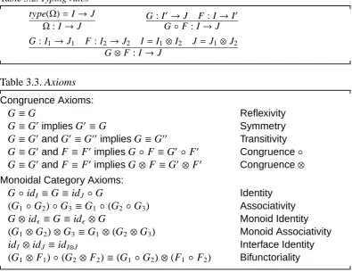
Table 3.2. Typing rules
type(Ω)= I →J Ω: I →J
G : I0→J F : I →I0 G◦F : I →J G : I1 →J1 F : I2→J2 I =I1⊗I2 J= J1 ⊗J2
[image:7.595.92.488.80.385.2]G⊗ F : I→ J
Table 3.3. Axioms
Congruence Axioms:
G≡G Reflexivity
G≡G0impliesG0 ≡G Symmetry
G≡G0andG0 ≡G00 impliesG≡G00 Transitivity
G≡G0and F ≡F0 impliesG◦ F ≡G0 ◦F0 Congruence◦
G≡G0and F ≡F0 impliesG⊗ F ≡G0 ⊗F0 Congruence⊗
Monoidal Category Axioms:
G◦idI ≡G ≡idJ ◦G Identity
(G1 ◦G2)◦G3 ≡G1 ◦(G2 ◦G3) Associativity
G⊗ id ≡G ≡id ⊗G Monoid Identity
(G1 ⊗G2)⊗G3 ≡G1 ⊗(G2 ⊗G3) Monoid Associativity
idI ⊗ idJ ≡ idI⊗J Interface Identity
(G1 ⊗ F1)◦(G2⊗ F2)≡ (G1◦G2)⊗(F1 ◦F2) Bifunctoriality
Intuitively, terms represent typed structures with a source and a target interface (G :
I → J). Structures can be placed one near to the other (horizontal composition) or
one inside the other (vertical composition). EachΩinΘhas a fixed type type(Ω)=
I → J. For each interface I, we assume a distinguished construct idI : I → I. The types of constructors, together with the rules in Tab. 3.2, determine the type of each term. Terms of type → J are called ground.
The term obtained by tensor is well typed when both corresponding tensors on source and target interface are defined, namely they are separated structures. On the other hand, composition is defined only when the two involved terms share a common interface. In the following, we consider only well typed terms.
Terms are defined up to the structural congruence≡ described in Tab. 3.3. It sub-sumes the axioms of the monoidal categories. All axioms are required to hold when-ever both sides are well typed. Throughout the paper, when using=or≡we imply that both sides are defined; and when we need to remark that a bigraphical expres-sion E is well given, we write (E)↓. Later on, the congruence will be refined to model specialised structures, such as place graphs, link graphs or bigraphs.
corresponds to the equality of the corresponding arrows.
Example 1 An intuitive example of bifunctorial terms is provided by located
re-sources. Every location is represented by a cell; every cell can contain a resource. Horizontal composition represents the merging of cells, and vertical composition combines the resources included in the cells. This model will provide a semantics to the logical operators we are defining, and will show that BiLog, although inspired by bigraphs, is not only connected to the bigraphical framework (cf. Ex. 2).
The set of resources is a monoidal structure (M, λ,·) freely generated by a set Λ of resource generators. The resource monoid may possibly be partial. In this case, the monoid of interfaces is the commutative monoid of ordinals (N,0,+), freely generated by{1}. We define the constructor λ : 1 → 1 for the neutral elementλ and a constructor a : 1 → 1 for each element a ∈ Λ. Every element repre-sents a cell, the constructor a reprerepre-sents a cell containing the resource generator
a. Table 3.4 outlines the two composition operators. The vertical composition ◦ between two cells a1 and a2 corresponds to combine – when possible – the two generators contained in the cells, thus producing the cell a1·a2 containing the resource a1·a2. This operation produces a cell m for every resource m ∈ M. The horizontal composition⊗consists of aligning two cells, thus producing lists of cells.
The terms generated by these settings are resources vectors Their inner and outer faces correspond to their size. The horizontal composition⊗ is in general the jux-taposition of vectors. Given the vectors m1 ... mn : n → n, of size n, and
m0
1 ... m 0 n0 : n
0 →
n0, of size n0, the composition⊗is formally defined as
m1 ... mn ⊗ m01 ... m
0 n0
def
= m1 ... mn m01 ... m
0 n0 .
The resulting vector is typed by (n+n0)→(n+n0), and has size n+n0.
The vertical composition ◦ is defined only between vectors with equal size, and corresponds to combine the resources cell by cell, as follows:
m1 ... mn ◦ m01 ... m0n
def
= m1·m01 ... mn·m0n .
The two operations satisfy the bifunctiorial property, which represents here the possibility to chose either to concatenate the vectors first and then to combine the resources, or vice versa. For cells, the bifunctorial property says
m1 ⊗ m2
◦ m3 ⊗ m4
=
m1 ◦ m3
⊗ m2 ◦ m4
.
The two terms above correspond to m1·m3 m2·m4 . The bifunctorial provides two possible normal forms: (i) the horizontal outermost a1 ◦. . .◦ an
⊗ . . . ⊗ am1 ◦. . .◦ amnm
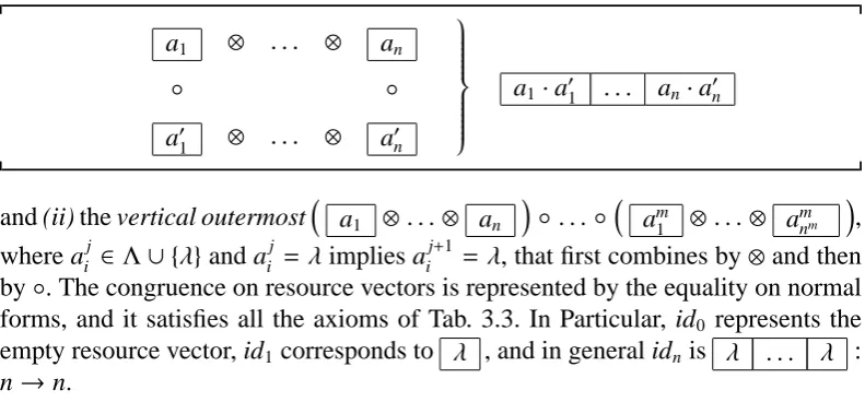
Table 3.4. Cell Compositions
a1 ⊗ . . . ⊗ an
◦ ◦
a0
1 ⊗ . . . ⊗ a 0 n
a1·a01 . . . an·a0n
and (ii) the vertical outermost a1 ⊗. . . ⊗ an
◦. . . ◦ am1 ⊗. . . ⊗ amnm
, where aij ∈Λ∪ {λ}and aij = λimplies aij+1 = λ, that first combines by⊗and then by◦. The congruence on resource vectors is represented by the equality on normal forms, and it satisfies all the axioms of Tab. 3.3. In Particular, id0 represents the empty resource vector, id1corresponds to λ , and in general idnis λ . . . λ :
n→n.
The properties of these particular terms depend strictly on the choice of the under-lying resource monoid, which can be either non-commutative (whenever ing sequences of resources, or ordered trees), or commutative (whenever consider-ing multisets of resources, or unordered trees), or partial (whenever dealconsider-ing with heaps). This example is rather limited, in the sense that inner and outer faces are forced to be equals, an there are only two kinds of constructors. The full general-ity will be reached with bigraphs. The aim of this model is to hint that BiLog can characterise models not directly based on bigraphs, as Ex. 2 will show.
3.2 Transparency
transparent or opaque, depending on the current policy, and the visibility in the logic, or in the query language, will be influenced by this.
When the model is dynamic, the reacting contexts, namely those with a possible temporal evolution, are specified with an activeness predicate. We may be tempted to identify transparency and activeness. Although these concepts collapse in some case, they are orthogonal in general. There may be transparent terms that are active, such as a public ‘browse-able’ directory; opaque terms that are active, such as an agent that hides its contents; passive transparent terms, such as a portable code; and passive opaque terms, such as controls encoding synchronisation.
More generally the transparency predicate prevents logical identification of terms. As an example, consider an XML document. We may want to restrict our attention to a particular set of nodes; we could, e.g., ignore data values when interested in the structure. In other situations, we may want a different logic focused on values, but not on node attributes.
Transparency is essentially a way to restrict the observational power of the struc-tural logic Notice that in general such a restriction of the observational power in the static logic does not imply a restriction of observational power in the dynamic counterpart. In fact, a next step modality may induce a ‘new’ intensionalisation of the controls by observing how the model evolves, as shown in [5] and [36].
3.3 Formulae
BiLog internalises the constructors of bifunctorial terms in the style of the ambi-ent logic [13]. Constructors appear in the logic as constant formulae, while tensor product and composition are expressed by connectives. Thus the logic presents two binary spatial operators. This contrasts with other spatial logics, with a single one: Spatial and Ambient Logics [4,13], with parallel composition A | B,
Separa-tion Logic [34], with separating conjuncSepara-tion A ∗ B, and Context Tree Logic [7],
with application K(P). Both the operators inherit the monoidal structure and non-commutativity properties from the model.
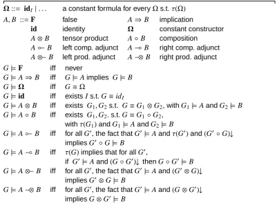
iden-Table 3.5. BiLog(M,⊗, ,Θ,≡, τ)
Ω::= idI |. . . a constant formula for everyΩs.t.τ(Ω) A,B ::=F false A⇒B implication
id identity Ω constant constructor A⊗ B tensor product A◦ B composition
AB left comp. adjunct A(B right comp. adjunct A⊗−B left prod. adjunct A−⊗B right prod. adjunct G|=F iff never
G|= A⇒B iff G|= Aimplies G|= B G|=Ω iff G≡Ω
G|=id iff existsIs.t.G≡idI
G|= A⊗ B iff exists G1,G2s.t. G≡G1⊗G2, withG1|=AandG2 |=B G|= A◦B iff exists G1,G2.s.t.G≡G1◦G2,
withτ(G1)andG1|= AandG2|=B
G|= AB iff for allG0,the fact thatG0 |=Aandτ(G0)and(G0◦G)↓ impliesG0 ◦G|=B
G|= A(B iff τ(G)implies that for allG0,
if G0 |=Aand(G◦G0)↓ thenG◦G0|= B G|= A⊗−B iff for allG0,the fact thatG0 |=Aand(G0 ⊗G)↓
impliesG0 ⊗G|= B
G|= A−⊗B iff for allG0,the fact thatG0 |=Aand(G⊗G0)↓
impliesG⊗G0|= B
tity idI for each interface I. The satisfaction of logical constants is simply the con-gruence to the corresponding constructor. The horizontal decomposition formula
A ⊗ B is satisfied by a term that can be decomposed as the tensor product of two
terms satisfying A and B respectively. The degree of separation enforced by⊗ be-tween terms plays a fundamental role in the various instances of the logic, notably link graph and place graph. The vertical decomposition formula A ◦ B is satisfied
by terms that can be the composition of terms satisfying A and B. We shall see that in some cases both connectives correspond to well known spatial ones. We define the left and right adjuncts for composition and tensor to express extensional proper-ties. The left adjunct A B expresses the property of a term to satisfy B whenever
inserted in a context satisfying A. Similarly, the right adjunct A( B expresses the
property of a context to satisfy B whenever filled with a term satisfying A. A similar description holds for⊗−and−⊗, the adjoints of⊗. Clearly these adjoints collapse whenever the tensor is commutative in the model.
Example 2 Consider the resource vectors defined in Ex. 1. When a BiLog formula
is interpreted in that context, it represents a class of resource vectors. For sake of simplicity, we assume that all this terms are transparent. Thus, when instantiated on these terms, BiLog provides a formula a for each constructor a . The semantics of a represents the class of all the terms whose normal form is the constructor
[image:11.595.87.489.85.382.2]re-spectively. For instance the formula a ⊗T is satisfied by all the resource vectors
having a as first cell. On the other hand, the formula a ◦ T implicitly says
that a resource vector is composed by a single cell containing a resource whose generators include a. In addition, if the resource monoid is not commutative, the previous formula says that the first element in the composition is actually a. The formula T ⊗ A ⊗ T characterises resources vectors with a subvector satisfying A.
In particular T ⊗ (A ◦ id1) ⊗ T means that one of the cells in the vector satisfied
A. Finally, if we use T ⊗ (T ◦ a ◦ T) ⊗ T says that the resource a appears
somewhere in the resource vector. More generally the formula id1 ◦ T means that the resource vector has size 1, then it is a simple sequence.
The formula Cell def
= id1 ◦(¬id1∧(¬(¬id1 ◦ ¬id1)) states that a resource vector is not empty and it is not composed by two not empty vectors, then it is a single cell. The Cell formula is useful to define two operators that correspond to the Kleene stars for the bigraphical combinators. Let a ⊗∗ def
= ¬T⊗Cell∧ ¬ a ⊗ T.
This formula is satisfied by resource vectors that are not composed by cells different from a . Thus a ⊗∗ characterises resource vectors of the kind a ⊗. . . ⊗ a ,
namely elements of the Kleene star generated by a and the composition⊗. This idea can be extended to a formula A:
A⊗∗ def
= ¬(T⊗(Cell∧ ¬A)⊗T) ; A◦∗ def
= ¬(T⊗(Cell∧ ¬A)⊗T).
A vector of resources satisfies A⊗∗if it is composed only by cells satisfying A.
3.4 Properties
Here we show some basic results about BiLog. In particular, we observe that, in presence of trivial transparency, the induced logical equivalence coincides with the structural congruence of the terms. Such a property is fundamental to describe, query and reason about bigraphical data structures, as e.g. XML (cf. §6). In other terms, BiLog is intensional in the sense of [36], namely it can observe internal structures, as opposed to the extensional logics used to observe the behaviour of dynamic system. Inspired by [24], it would be possible to study a fragment of BiLog without the intensional operators⊗,◦, and constants.
The lemma below states that the relation|=respects the congruence.
Lemma 1 (Congruence preservation) For every couple of terms G and G0, if G |=
A and G ≡G0 then G0 |= A.
Proof. Induction on the structure of the formula, by recalling that the congruence
Case F. Nothing to prove.
CaseΩ. By hypothesis G|= Ωand G≡G0. By definition G ≡Ωand by transitivity
G0 ≡Ω, thus G0 |=Ω.
Case id. By hypothesis G |= id and G ≡ G0. Hence there exists an I such that
G0 ≡G≡id
I and so G0 |=id.
Case A⇒ B. By hypothesis G |= A ⇒ B and G ≡ G0. This means that if G |= A then G|= B. By induction if G0 |= A then G|= A. Thus if G0 |= A then G |= B and
again by induction G0 |= B.
Case A⊗ B. By hypothesis G|= A⊗ B and G ≡G0. Thus there exist G
1, G2 such that G0 ≡G≡G1⊗G2and G1 |= A and G2|= B. Hence G0 |= A⊗ B.
Case A◦B. By hypothesis G |= A◦ B and G ≡ G0. Thus there exist G
1, G2 such that G0 ≡G≡G
1◦G2andτ(G1) and G1|=A and G2 |= B. Hence G0 |= A◦B.
Case A B. By hypothesis G|= A B and G≡G0. Thus for every G00 such that
G00 |= A and τ(G00) and (G00 ◦G)↓ it holds G00 ◦ G |= B. Now G ≡ G0 implies
G00 ◦G ≡ G00 ◦ G0; moreover the congruence preserves typing, so (G00 ◦G0)↓. By induction G00 ◦G0 |= B, then conclude G0|=A B.
Case A( B. Ifτ(G0) is not verified, then G0 |= A
( B trivially holds. Suppose
τ(G0) to be verified. As G ≡G0 and transparency preserves congruence,τ(G) is verified as well. By hypothesis for each G00 satisfying A such that (G ◦G00)↓ it holds G ◦ G00 |= B, and by induction G0 ◦ G00 |= B, as G ≡ G0 and (G ◦ G00)↓ implies (G0 ◦G00)↓ and G◦G00 ≡G0 ◦G00. This proves G0 |= A
( B.
Case A⊗−B (and symmetrically A−⊗ B). By hypothesis G |= A ⊗− B and G ≡
G0. Thus for each G00 such that G00 |= A and (G00 ⊗ G)↓ then G00 ⊗G |= B. Now
G ≡ G0 implies G00 ⊗ G ≡G00 ⊗G0, again the congruence must preserve typing so (G00 ⊗ G0)↓. Thus by induction G00 ⊗ G0 |= B. The generality of G00 implies
G0 |= A⊗−B. 2
BiLog induces a logical equivalence =L on terms in the usual sense. We say that
G1 =LG2 if for every formula A, G1 |= A implies G2 |= A and vice versa. It is easy to prove that the logical equivalence corresponds to the congruence in the model if the transparency predicate is true for every term.
Theorem 1 (Logical equivalence and congruence) When the transparency pred-icate is always true, then G=LG0if and only if G ≡G0 for every term G, G0.
Proof. The forward direction is proved by defining the characteristic formula for
terms, as every term can be expressed as a formula. In fact, the transparency pred-icate is total, hence every constant term corresponds to a constant formula. The converse is a direct consequence of Lemma 1. 2
Table 4.1. Derived Operators
T,∧, ∨, ⇔,⇐,¬ Classical operators AI def
= A◦idI Constraining the source to beI A→J def
= idJ ◦A Constraining the target to beJ AI→J def
= (AI)→J Constraining the type to beI→ J A◦I B def
= A◦idI ◦B Composition with interfaceI
AJ Bdef= A→J B Contexts withJ as target guarantee A(I B def= AI (B Composing with terms havingI as source A B def
= ¬(¬A⊗ ¬B) Dual of tensor product A•B def
= ¬(¬A◦ ¬B) Dual of composition
AB def= ¬(¬A¬B) Dual of composition left adjunct AB def= ¬(¬A(¬B) Dual of composition right adjunct A∃⊗ def
= T⊗A⊗T Some horizontal term satisfiesA A∀⊗ def
= F A F Every horizontal term satisfiesA A∃◦ def
= T◦A◦T Some vertical term satisfiesA A∀◦ def
= F•A•F Every vertical term satisfiesA ◊A def
= (T◦A) Somewhere modality (on ground terms)
◊A def
= ¬ ◊¬A Anywhere modality (on ground terms)
That means we can find an equivalence relation between trees that is ‘tuned’ byτ: the moreτcovers, the less the equivalence distinguishes. This relation will be better understood when we instantiate the logic to particular terms. A possible definition of transparency will be provided in §5.6.
4 BiLog: derived operators
Table 4.1 outlines several operators that can be derived in BiLog. The classical operators and those constraining the interfaces are self-explanatory. The ‘dual’ op-erators are worth explaining. The formula A B is satisfied by terms G such that for
every possible decomposition G≡G1 ⊗G2either G1 |= A or G2 |= B. For instance,
A A describes terms where A is true in, at least, one part of each⊗-decomposition. The formula F (T→I ⇒ A) F describes those terms where every component with outerface I satisfies A. Similarly, the composition A•B expresses structural
prop-erties universally quantified on every◦-decomposition. Both these connectives are useful to specify security properties or types.
The adjunct dual A B describes terms that can be inserted into a particular
con-text satisfying A to obtain a term satisfying B, it is a sort of existential quantification on contexts. For instance (Ω1∨Ω2) A describes the union between the class of two-region bigraphs (with no names in the outerface) whose merging satisfies A, and terms that can be inserted either in Ω1 or Ω2 resulting in a term satisfying A. Similarly the dual adjunct A B describes contextual terms G such that there
The formulae A∃⊗, A∀⊗, A∃◦,and A∀◦correspond to quantifications on the horizon-tal/vertical structure of terms. For instance Ω∀◦ describes terms that are a finite (possibly empty) composition of simple terms Ω. Next section discusses spatial modalities ◊and◊.
Following lemma states a first property involving the derived connectives, by prov-ing that the interfaces for transparent terms can be observed.
Lemma 2 (Type observation) For every term G, it holds: G |= AI→J if and only if
G : I → J and G |= A andτ(G).
Proof. For the forward direction, assume that G |= AI→J, then G ≡ idJ ◦ G0 ◦ idI with G0 |= A and τ(G0). Now, idJ ◦ G0 ◦ idI : I → J. By Lemma 1: G : I →
J and G |= A and τ(G). The converse is a direct consequence of the semantics
definition. 2
Thanks to the derived operators involving interfaces, the equality between inter-faces, I = J, is derivable by⊗and⊗−, as
T⊗ (id∧(idI ⊗−idJ)). (1)
Whenever a bigraph satisfies such a formula, the interfaces I and J are equal. To gather the basic idea, assume the bigraph G satisfies (1). This means that G≡G1⊗
G2with G1 |= T and G2 |= id∧(idI ⊗− idJ). By definition, the latter is equivalent to G2 ≡ and G2 |= idI ⊗− idJ. Then G ≡ G1 and |= idI ⊗− idJ, by Lemma 1. Hence ⊗ idI |= idJ, that entails idI ≡ idJ. Clearly, the last equality holds only if I = J. By reversing the reasoning, it is easy to see that whenever I = J, every
bigraph satisfies (1).
4.1 Somewhere modality
The idea of sublocation,vdefined in [14], can be extended to the bigraphical terms. A sublocation corresponds to a subterm and it is formally defined on ground terms as follows. The definition of sublocation makes sense only for ground terms, as the structure of ‘open’ terms (i.e., with holes) is not known a priori. Formally it is defined as follows.
Definition 1 (Sublocation) Given two terms G : → J and G0 : → J0, term G0 is defined to be a sublocation for G, and write G0 vG, inductively by:
• G0 vG, if G0 ≡G;
• G0 vG, if G≡G1⊗G2, with G0 vG1or G0vG2; • G0 vG, if G≡G
This relation, introduce a “somewhere” modality in the logic. Intuitively, a term sat-isfies “somewhere”A whenever one of its sublocations satsat-isfies A. Rephrasing the semantics given in [14], a term ground term G satisfies the formula “somewhere”A if and only if there exists G0 v G such that G0 |= A. Quite surprisingly, such a
modality is expressible in the logic. In fact, in case of ground terms, the previous requirement is the semantics of the derived connective ◊, defined in Tab. 4.1.
Proposition 1 For every ground term G:
G |= ◊A if and only if there exists G0 vG such that G0 |= A.
Proof. First prove a supporting property characterising the relation between a term
and its sublocations.
Property 1 For every ground term G and G0, it holds: G0 v G if and only if there
exists a term C such thatτ(C) and G ≡C◦G0.
The direction from right to left is a simple application of Definition 1. The direction from left to right is proved by induction on Definition 1. For the basic step, the implication clearly holds if G0 vG in case G0 ≡G. The inductive step distinguishes two cases.
If G0 vG is due to the fact that G ≡ G
1 ⊗G2, with G0 vG1 or G0 v G2. Without loss of generality, assume G0 vG
1. The induction says that there exists C such that τ(C) and G1 ≡C ◦G0. Hence, G≡ (C ◦G0)⊗G2. Now the typing is: C : IC → JC;
G0 : → I
C; G2 : → J2; and G : ⊗ → JC ⊗ J2. So G≡(C ◦G0)⊗(G2 ◦id). As the interface is the neutral element for the tensor product between interfaces, compose C ⊗ G2 : IC ⊗ → JC ⊗ J2, and G0 ⊗ id : ⊗ → IC ⊗ . Hence the term (C ⊗ G2) ◦ (G0 ⊗ id) is defined. Note thatτ(C ⊗ G2) is true,as τ(G2) is verified since G2 : → J2 andτ(C) is true by induction. Hence, by bifunctoriality property, conclude G ≡(C ⊗G2)◦G0, withτ(C ⊗G2), as aimed.
On the other hand, if G0 v G is due to the fact that G ≡ G
1 ◦ G2, withτ(G1) and
G0 v G2. The induction says that there exists C such that τ(C) and G2 ≡ C ◦ G0. Hence, G ≡G1 ◦(C ◦G0). Conclude G≡(G1 ◦C)◦G0, withτ(G1 ◦C).
Suppose now that G |= ◊A, this means that G |= (T ◦ A). According to Tab. 4.5,
this means that there exist C and G0 such that G0 |= A and τ(C), and G ≡ C ◦ G0. Finally, by Property 1, this means G0 vG and G0 |= A.
2
The everywhere modality (◊) is dual to ◊. A term satisfies the formula◊ A if each
4.2 Logical properties deriving form categorical axioms
For every axiom of the model, the logic proves a corresponding property. In partic-ular, the bifunctoriality property is expressed by formulae
(AI ◦B→I)⊗(A0J ◦B 0
→J)⇔(AI ⊗ A0J)◦(B→I ⊗ B0→J) valid when (I⊗ J)↓.
In general, given two formulae A,B we say that A yields B, and we write A ` B,
if for every term G it is the case that G |= A implies G |= B. Moreover, we write Aa` B to say both A` B and B` A.
Assume that I and J are two interfaces such that their tensor product I ⊗ J is
defined. Then, the bifuctoriality property in the logic is expressed by (AI ◦B→I)⊗(A0J ◦B
0
→J)a`(AI ⊗A0J)◦(B→I ⊗ B0→J). (2)
Proposition 2 Whenever (I ⊗ J)↓, the equation (2) holds in the logic.
Proof. Prove separately the two way of the satisfaction. First prove (AI ◦ B→I) ⊗ (A0J ◦ B0→J) ` (AI ⊗ A0J) ◦ (B→I ⊗ B0→J). Assume that G |= (AI ◦ B→I) ⊗ (A0J ◦
B0
→J). This means that there exist G
0 : I0 → I00, G00 : J0 → J00 such that I0 ⊗ J0 and
I00 ⊗ J00 are defined, and G ≡G0 ⊗ G00, with G0 |= AI ◦ B→I and G00 |= A0J ◦ B 0 →J. Now, G0 |= AI ◦ B→I means that there exist G1 and G2 such that (i) G0 ≡G1 ◦G2,
(ii) G1 : I → J0, with τ(G1) and G1 |= A, and (iii) G2 : I0 → I, with G2 |= B. Similarly, G00 |= A0J ◦ B0→J means (i) G00 ≡ G01 ◦ G02 and (ii) G01 : J → J00, with τ(G0
1) and G 0 1 |= A
0
, and (iii) G02 : I00 → J, with G2 |= B0. In particular, conclude
G ≡ (G1 ◦ G2) ⊗ (G01 ◦ G02). As I ⊗ J is defined, (G1 ⊗ G01) ◦ (G2 ⊗ G02) is an admissible composition. The bifunctoriality property implies G ≡ (G1 ⊗ G01) ◦ (G2 ⊗ G02). Moreoverτ(G1 ⊗ G01), as τ(G1) and τ(G01). Hence conclude that G |= (AI ⊗ A0J)◦(B→I ⊗ B0→J), as required.
For the converse, prove (AI ⊗ A0J) ◦ (B→I ⊗ B0→J) ` (AI ◦ B→I) ⊗ (A 0 J ◦ B
0 →J). Assume that G |= (AI ⊗ A0J) ◦ (B→I ⊗ B0→J). By following the same lines as before, deduce that G ≡ (G1 ⊗ G01) ◦ (G2 ⊗ G02), where (i) τ(G1 ⊗ G01), (ii)
G1 : I → J0such that G1|= A, (iii) G01 : J → J00such that G01|= A0, (iv) G2 : I0 → I such that G2 |= B, and (v) G02 : I
00 →
J such that G2 |= B0. Also in this case, the tensor product of the required interfaces can be performed. Hence compose (G1 ◦ G2) ⊗ (G10 ◦ G02). Again, the bifunctoriality property implies G ≡ (G1 ◦
G2) ⊗ (G01 ◦ G 0
2). Finally, by observing thatτ(G1 ⊗ G01) implies τ(G1) andτ(G01), deduce G1 ◦ G2 |= (AI ◦ B→I) and (G01 ◦ G02) |= (A0J ◦ B0→J). Then conclude
Table 5.1. Additional Axioms for Place Graphs Structural Congruence
Symmetric Category Axioms:
γm,0 ≡idm Symmetry Id
γm,n ◦γn,m≡idm⊗n Symmetry Composition γm0,n0 ◦(G⊗F)≡(F⊗G)◦γm,n Symmetry Monoid Place Axioms:
join◦(1⊗id1)≡id1 Unit
join◦(join⊗id1)≡join◦(id1 ⊗join) Associativity join◦γ1,1 ≡join Commutativity
5 BiLog: instances and encodings
In this section BiLog is instantiated to describe place graphs, link graphs and bi-graphs. A spatial logic for bigraphs is a natural composition of a place graph logic, for tree contexts, and a link graph logic, for name linkings. Each instance admits an embedding of a well known spatial logic.
5.1 Place Graph Logic
Place graphs are essentially ordered lists of regions hosting unordered labelled trees with holes, namely contexts for trees. Tree labels correspond to controlsK : 1→ 1 belonging to a fixed signatureK. The monoid of interfaces is the monoid (ω,+,0) of finite ordinals m,n. Ordinals represent the number of holes and regions of place
graphs. Place graph terms are generated from the set
Θ = {1 : 0→ 1,idn : n→n,join : 2→1, γm,n : m+n→n+m} ∪ K The only structured terms are the controls K, representing regions containing a single node with a hole inside. All the other constructors are placings and represent trees m → n with no nodes: the place identity idn is neutral for composition; the constructor 1 represents a barren region; join is a mapping of two regions into one; γm,n is a permutation that interchanges the first m regions with the following n. The structural congruence ≡ for place graph terms is refined, in Tab. 5.1, by the usual axioms for symmetry of γm,n and by the place axioms that essentially turn the operation join ◦ ( ⊗ ) in a commutative monoid with 1 as neutral element. In particular, the places generated by composition and tensor product fromγm,nare
permutations. A place graph is prime if it has type I → 1, namely it has a single region.
Example 3 The term
G def
is a place graph of type 2→2, on a signature containing service, name, description, and push. It represents an ordered pair of trees. The first tree is labelled service and has name and description as (unordered) children, both children are actually con-texts with a single hole. The second tree is ground as it has a single node without children. The term G is congruent to (service⊗ push)◦(join⊗ 1)◦(description⊗
name).Such a contextual pair of trees can be interpreted as semi-structured partial data (e.g. an XML message, a web service descriptor) that can be filled by com-position. The order among holes is a major issue in the composition, for instance, (K1 ⊗ K2) ◦(K3 ⊗1) is different from (K1 ⊗ K2)◦ (1⊗ K3), as nodeK3plugs into
K1in the first case, and insideK2in the second one.
Fixed the transparency predicate τ on each control in K, the Place Graph Logic PGL(K, τ) is BiLog(ω,+,0,≡,K ∪ {1,join, γm,n}, τ). We assume the transparency predicateτto hold for join andγm,n. Theorem 1 can be extended to PGL, thus such a logic can describe place graphs precisely. The logic resembles a propositional spatial tree logic, in the style of [6]. The main differences are that PGL models contexts of trees and that the tensor product is not commutative, unlike the parallel composition in [6], and it enables the modelling of the order among regions. The logic can express a commutative separation by using join and the tensor product, namely the parallel composition operator A|Bdef
=join◦(A→1 ⊗ B→1).At the term level, this separation, which is purely structural, corresponds to join ◦ (P1 ⊗ P2), that is a total operation on all prime place graphs. More precisely, the semantics says that P |= A | B means that there exist P1 : I1 → 1 and P2 : I2 → 1 such that:
P≡ join◦(P1 ⊗P2) and P1 |= A and P2 |= B.
5.2 Encoding STL
Not surprisingly, prime ground place graphs are isomorphic to the unordered trees modelling the static fragment of ambient logic. Here we show that, when the trans-parency predicate is always verified, BiLog restricted to prime ground place graphs is equivalent to the propositional Spatial Tree Logic of [6] (STL in the following). The logic STL expresses properties of unordered labelled trees T constructed from the empty tree 0, the labelled node containing a tree a[T ], and the parallel composi-tion of trees T1|T2, as detailed in Tab. 5.2. Labels a are elements of a denumerable set Λ. STL is a static fragment of the ambient logic [13] and it is characterised by the usual classical propositional connectives, the spatial connectives 0, a[A],
A|B, and their adjuncts A@a, A.B. The language of the logic and its semantics is
outlined in Tab. 5.3.
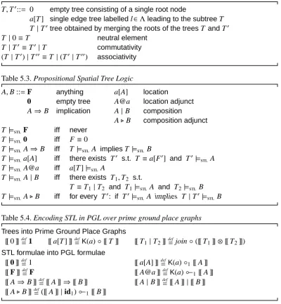
Table 5.2. Information tree Terms (overΛ) and congruence T,T0::= 0 empty tree consisting of a single root node
a[T ] single edge tree labelledl∈Λleading to the subtreeT T |T0tree obtained by merging the roots of the treesT andT0 T |0≡T neutral element
T |T0 ≡T0|T commutativity
[image:20.595.90.491.84.518.2](T |T0)|T00 ≡T |(T0|T00) associativity
Table 5.3. Propositional Spatial Tree Logic
A,B ::=F anything a[A] location
0 empty tree A@a location adjunct A⇒B implication A|B composition
A.B composition adjunct T |=F iff never
T |=0 iff F ≡0
T |=A⇒B iff T |=A impliesT |=B
T |=a[A] iff there exists T0 s.t. T ≡a[F0] and T0|= A T |=A@a iff a[T ]|=A
T |=A|B iff there exists T1,T2 s.t.
T ≡T1|T2 and T1|=A and T2 |= B
T |=A.B iff for every T0: if T0|=A implies T |T0|=B
Table 5.4. Encoding STL in PGL over prime ground place graphs
Trees into Prime Ground Place Graphs
[[ 0 ]]def
=1 [[ a[T ] ]]def
=K(a)◦[[ T ]] [[ T1|T2]]def=join◦([[ T1]]⊗[[ T2]]) STL formulae into PGL formulae
[[ 0 ]]def
=1 [[ a[A] ]]def
=K(a)◦1 [[ A ]]
[[ F ]]def
=F [[ A@a ]]def
= K(a)1 [[ A ]]
[[ A⇒B ]]def
= [[ A ]]⇒[[ B ]] [[ A|B ]]def
=[[ A ]]|[[ B ]] [[ A.B ]]def
=([[ A ]]|id1)1[[ B ]]
The monoidal properties of parallel composition are guaranteed by the symmetry and unit axioms of join. The equations are self-explanatory once we remark that: (i) the parallel composition of STL is the structural commutative separation of PGL;
(ii) tree labels can be represented by the corresponding controls of the place graph; (iii) location and composition adjuncts of STL are encoded by the left composition
adjunct, as they add logically expressible contexts to the tree. This encoding is actually a bijection tree to prime ground place graphs. In fact, there is an inverse
encoding ([ ]) for prime ground place graphs in trees defined on the normal forms
of [30].
The theorem of discrete normal form in [30] implies that every ground place graph
g : 0→1 can be expressed as
where every Mjis a molecular prime ground place graph of the form M =K(a)◦g, with ar(K(a)) = 0. As an auxiliary notation, joinn is inductively defined as join0 def
= 1, and joinn+1 def
= join◦(id1 ⊗joinn). The bifunctoriality property implies
joinn◦(M0 ⊗. . . ⊗ Mn−1)≡
≡join◦(M0 ⊗(join◦(M1 ⊗ (join◦(. . . ⊗(join◦(Mn−2 ⊗ Mn−1))))))). The work in [30] says that the normal form in (3) is unique, up to permutations. For every prime ground place graph, the inverse encoding ([ ]) considers its discrete normal form and it is inductively defined as follows
([ join0]) def
= 0
([K(a)◦q ]) def
= a[ ([ q ]) ]
([ joins◦(M0 ⊗. . . ⊗ Ms−1) ]) =def ([ M0])|. . .|([ Ms−1])
The encodings [[ ]] and ([ ]) are one the inverse of the other, hence they give a bijec-tion from trees to prime ground place graphs, which is fundamental in the proof of the following theorem.
Theorem 2 (Encoding STL) For each tree T and formula A of STL:
T |=A if and only if [[ T ]]|= [[ A ]].
Proof. The theorem is proved by structural induction on STL formulae. The
trans-parency predicate is not considered here, as it holds on every control. The ba-sic step deals with the constants F and 0. Case F follows by definition. For the case 0, [[ T ]] |= [[ 0 ]] means [[ T ]] |= 1, that by definition is [[ T ]] ≡ 1 and so
T ≡([ [[ T ]] ])≡ ([ 1 ])def
= 0, namely T |=0.
The inductive steps deal with connectives and modalities.
Case A⇒ B. Assuming [[ T ]]|= [[ A⇒ B ]] means [[ T ]]|= [[ A ]]⇒[[ B ]]; by defi-nition this says that [[ T ]]|= [[ A ]] implies [[ T ]]|= [[ B ]]. By induction hypothesis, this is equivalent to say that T |= A implies T |= B, namely T |=A⇒ B. Case a[A]. Assuming [[ T ]]|= [[ a[A] ]] means [[ T ]]|=K(a)◦1 ([[ A ]]). This amount
to say that there exist G : 1 → 1 and g : 0 → 1 such that [[ T ]] ≡ G ◦ g and G |= K(a) and g |= [[ A ]], that is [[ T ]] ≡ K(a) ◦ g with g |= [[ A ]]. Since the encoding is bijective, this is equivalent to T ≡ ([K(a) ◦ g ]) def
= a[([ g ])] with g|= [[ A ]]. Since g : 0 → 1, the induction hypothesis says that ([ g ]) |= A. Hence
it is the case that T |= a[A].
[[ a[T ] ]]|=[[ A ]]. By induction hypothesis, this is a[T ]|= A. Hence T |= A@a
by definition.
Case A|B. Assuming that [[ T ]] |= [[ A | B ]] means [[ T ]] |= [[ A ]] | [[ B ]]. This is equivalent to say that [[ T ]] |= join ◦ ([[ A ]]→1 ⊗[[ B ]]→1), namely there exist
g1,g2 : 0 →1 such that [[ T ]] ≡ join ◦(g1 ⊗ g2) and g1 |= [[ A ]] and g2 |= [[ B ]]. As the encoding is bijective this means that T ≡ ([ g1])|([ g2]), and the induction hypothesis says that ([ g1])|= A and ([ g2])|= B. By definition this is T |= A|B. Case A.B. Assuming that [[ T ]]|=[[ A.B ]] means [[ T ]]|=join([[ A ]]⊗ id1))1 [[ B ]], namely for every G : 1 → 1 such that G |= join([[ A ]]⊗ id1) it holds
G ◦[[ T ]] |= [[ B ]]. Now, G : 1 → 1 and G |= join([[ A ]]⊗ id1) means that there exists g : 0 → 1 such that g|= [[ A ]] and G≡ join(g⊗ id1). Hence it is the case that for every g : 0→1 such that g|= [[ A ]] it holds join(g⊗id1)◦[[ T ]]|=[[ B ]], that is join(g⊗[[ T ]]) |= [[ B ]] by bifunctoriality property. Since the encoding is a bijection, this is equivalent to say that for every tree T0such that [[ T0]]|=[[ A ]] it holds join([[ T0]]⊗ [[ T ]]) |= [[ B ]], that is [[ T0 | T ]] |= [[ B ]]. By induction hypothesis, for every T0 such that T0 |= A it holds T0 | T |= B, that is the
semantics of T |= A.B. 2
Differently from STL, PGL can also describe structures with several holes and re-gions. In §6 we show how PGL describes contexts of tree-shaped semistructured data. Consider, for instance, a function taking two trees and returning the tree ob-tained by merging their roots. Such a function is represented by the term join, which solely satisfies the formula join. Similarly, the function that takes a tree and encap-sulates it inside a node labelled byK, is represented by the termKand captured by the formulaK. Moreover, the formula join◦(K⊗ (T◦id1)) expresses all contexts of form 2 →1 that place their first argument inside aKnode and their second one as a sibling of such node.
5.3 Link Graph Logic (LGL).
Fixed a denumerable set of namesΛ, we consider the monoid (Pfin(Λ),],∅), where Pfin( ) is the finite powerset operator and]is the subset disjoint union. Link graphs are the structures arising from such a monoid. They can describe nominal resources, common in many areas: object identifiers, location names in memory structures, channel names, and ID attributes in XML documents. The fact that names cannot be implicitly shared does not mean that we can refer to them or link them explicitly (e.g. object references, location pointers, fusion in fusion calculi, and IDREF in XML files). Link graphs describe connections between resources performed by means of names, that are references.
Wiring terms are a structured way to map a set of inner names X into a set of outer names Y. They are generated by the constructors: /a : {a} → ∅ and a/
X :
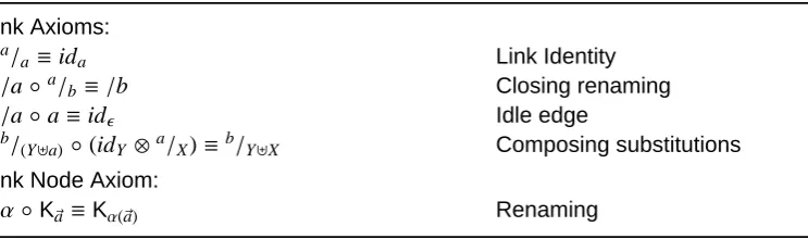
Table 5.5. Additional Axioms for Link Graph Structural Congruence
Link Axioms: a/
a≡ida Link Identity /a◦a/b≡/b Closing renaming /a◦a≡id Idle edge
b/
(Y]a) ◦(idY ⊗a/X)≡b/Y]X Composing substitutions Link Node Axiom:
α◦K~a ≡Kα(~a) Renaming
a/
X associates all the names in the set X to the name a. We denote wirings by ω, substitutions by σ, τ, and bijective substitutions, dubbed renamings, by α, β. Substitution can be specialised in: a def
= a/
∅ and a ← b def= a/{b} and a ⇔ b def= a/
{a,b}. The constructor a represents the introduction of name a, the term a ← b corresponds to rename b to a, and a⇔b links, or fuses, a and b to name a.
Given a signatureK of controlsKwith arity function ar(K) we generate link graphs from wirings and the constructor K~a : ∅ → ~a with~a = a1, . . . ,ak, K ∈ K, and
k= ar(K). The controlK~arepresents a resource of kindKwith named ports~a. Any ports may be connected to other node ports via wiring compositions.
In this case, the structural congruence ≡ is refined as outlined in Tab. 5.5 with obvious axioms for links, modelling α-conversion and extrusion of closed names. We assume the transparency predicateτtrue on wiring constructors.
Fixed the transparency predicate τ for each control inK, the Link Graph Logic LGL(K, τ) is BiLog(Pfin(Λ),],∅,≡,K ∪ {/a,a/X}, τ). Theorem 1 extends to LGL: the logic describes the link graphs precisely. The logic expresses structural spatial-ity for resources and strong spatialspatial-ity (separation) for names, and it can therefore be viewed as a generalisation of Separation Logic for contexts and multi-ports lo-cations. On the other side, the logic can describe resources with local (hidden or private) names between resources, and in this sense the logic is a generalisation of Spatial Graph Logic [10]: it is sufficient to consider the edges as resources.
Moreover, if we consider identity as a constructor, it is possible to define
a← bdef
=(a⇔b)◦(a⊗idb).
In LGL the formula A⊗ B describes a decomposition into two separate link graphs,
sharing neither resources, nor names, nor connections, that satisfy A and B respec-tively. Since it is defined only on link graphs with disjoint inner/outer sets of names, the tensor product is a kind a spatial/separation operator, in the sense that it
sepa-rates the model into two distinct parts that cannot share names.
resources, we need to make the sharing explicit, and the sole way to do that is through the link operation. We therefore need a way to first separate the names occurring in two wirings as to apply the tensor, and then link them back together. As a shorthand, if W : X → Y and W0 : X0 → Y0 with Y ⊂ X0, we write [W0]W for (W0 ⊗ id
X0\Y) ◦ W and if~a = a1, . . . ,an and~b = b1, . . . ,bn, we write~a ← ~b for a1 ← b1 ⊗ . . . ⊗ an ← bn, similarly for~a ⇔ ~b. From the tensor product it is possible to derive a product with sharing on~a. Given G : X → Y and G0 : X0 →Y0
with X∩X0 = ∅, we choose a list~b (with the same length as~a) of fresh names. The composition with sharing~a is
G ⊗~a G0 def
=[~a⇔~b]([~b←~a]G ⊗G0).
In this case, the tensor product is well defined since all the common names~a in W are renamed to fresh names, while the sharing is re-established afterwards by
linking the~a names with the~b names.
By extending this sharing to all names we define the parallel composition G|G0as a total operation. However, such an operator does not behave ‘well’ with respect to the composition, as shown in [30]. In addition a direct inclusion of a correspond-ing connective in the logic would impact the satisfaction relation by expandcorrespond-ing the finite horizontal decompositions to the boundless possible name-sharing decom-positions. (This may be the main reason why logics describing models with name closure and parallel composition are undecidable [18].) This is due to the fact that the set of names shared by a parallel composition is not known in advance, and therefore parallel composition can only be defined by using an existential quantifi-cation over the entire set of shared names.
Names can be internalised and effectively made private to a bigraph by the closure operator/a. The effect of composition with/a is to add a new edge with no public
name, and therefore to make a disappear from the outerface, and be completely hidden to the outside. Separation is still expressed by the tensor connective, which not only separates places, but also makes sure that no edge – whether visible or hidden – crosses the separating line.
As a matter of fact, without name quantification it is not possible to build formulae that explore a link, since the latter has the effect of hiding names. For this task, we employ the name variables x1, ...,xnand the fresh name quantification N . in the style of Nominal Logic [35]. The semantics is defined as
G|= N x1. . .xn.A iff there exist a1. . .an <fn(G)∪fn(A)
such that G |= A{x1. . .xn ←a1. . .an},
where A{x1. . .xn ←a1. . .an}is the usual variable substitution.