Probabilistic based characterisation of the mechanical properties of CFRP laminates

Submitted to Construction and Building Materials

PROBABILISTIC-BASED CHARACTERISATION OF THE MECHANICAL

1

PROPERTIES OF CFRP LAMINATES

2

S. Gomes1, D. Dias-da-Costa*,2, L.A.C. Neves3, S.A. Hadigheh2, P. Fernandes4, E. Júlio5 3

*_{corresponding author (Email: [email protected])}

4

1_{ISISE, Department of Civil Engineering, University of Coimbra, Rua Luís Reis Santos, 3030–788}

5

Coimbra, Portugal. 6

2_{School of Civil Engineering, The University of Sydney, Sydney, NSW 2006, Australia.}

7

3_{Centre for Risk and Reliability Engineering, University of Nottingham, Faculty of Engineering,}

8

University Park, United Kingdom. 9

4_{Civil Engineering Department, Instituto Politécnico de Leiria, Portugal.}

10

5_{CEris-ICIST, DECivil, Instituto Superior Técnico, Universidade de Lisboa, Av. Rovisco Pais,}

11

1049-001 Lisboa, Portugal 12

Abstract

13

Fibre reinforced polymer (FRP) composites have been increasingly used worldwide in the 14

strengthening of civil engineering structures. As FRP becomes more common in structural 15

strengthening, the development of probability-based limit state design codes will require accurate 16

models for the prediction of the mechanical properties of the FRPs. Existing models, however, are 17

based on small sample sizes and ignore the importance of the tail region for analyses and design. 18

Addressing these limitations, this paper presents a probabilistic-based characterisation of the 19

mechanical properties of carbon FRP (CFRP) laminates using a large batch of tension tests. The 20

analysed specimens were pre-cured laminates of carbon fibres embedded in epoxy matrices, which 21

is the most commonly used laminate for the strengthening concrete beams and slabs. Based on the 22

existing data, probabilistic models and correlations were established for the Young's modulus, 23

ultimate strain and tensile strength. Analyses demonstrate the suitability of the Weibull distribution 24

for the estimation of CFRP properties. Results also show that the statistical characterisation of the 25

mechanical properties should be performed with a focus on the tail region. The proposed 26

distributions constitute a set of validated probabilistic models that can be used for performing 27

reliability analyses of structures strengthened with CFRP laminates. 28

29

Keywords: CFRP laminates; strengthening of structures; Mechanical properties; Probabilistic

30

models. 31

*Revised Manuscript

2

1. Introduction

32

During the last decades, externally bonded reinforcement (EBR) of fibre-reinforced polymers 33

(FRP) has become a common technique to strengthen and upgrade civil engineering structures. FRP 34

is usually used in the form of wet lay-up sheets or pre-fabricated laminates due to their simplicity 35

and lower capital cost. The former system is based on the direct application of fibre sheets saturated 36

with resin, whereas the second uses pre-fabricated cured strips. There are also automated techniques 37

using vacuum (e.g. resin infusion techniques) or vacuum and heat (e.g. heated vacuum bag only) for 38

impregnation of fibres [1-3]. The characteristics of the FRP, namely its lightweight, high durability 39

in aggressive environments, ease of installation and cost effectiveness, are quite competitive for 40

strengthening purposes and constitute a good alternative to more traditional methods and materials, 41

such as EBR using steel plates or concrete jacketing [1]. There are several examples where FRPs 42

were used to increase the flexural, shear or axial capacity of structural members, such as beams, 43

slabs, columns, or joints [4-8]. 44

The growing interest in FRP composites resulted in the development of several design guidelines 45

(e.g. CEB-FIB [9], TR-55 [10], CNR [11] and ACI 440.2R-08 [12]). These, however, are not 46

presently at a level of development comparable to those used in structural concrete and steel design. 47

Considering the uncertainties present in FRP applications, new guidelines are required to develop 48

probability-based limit state design codes and to support the acceptance of FRP materials in civil 49

engineering [13, 14]. Despite previous reliability studies (e.g. Ellingwood [13], Plevris, 50

Triantafillou [15], Okeil, El-Tawil [16], Monti and Santini [17], Atadero, Lee [18], Atadero and 51

Karbhari [19], Okeil, Belarbi [20], and Ali, Bigaud [21]) having addressed some of these 52

uncertainties, the statistical information is still limited in the development of more accurate 53

probabilistic models. 54

A variety of factors affect the properties of FRP after manufacturing which create a degree of 55

3

Weibull and Gamma distributions to analyse the probabilistic properties of field-manufactured wet 57

lay-up carbon and glass composites. Six sets, composed by one, three or four subsets resulting in 58

903 samples, were considered to assess the tensile strength, the Young's modulus and the laminate 59

thickness. Despite the large number of samples used, the need to divide them in smaller subsets of 60

different properties and manufacturing processes led to a significant reduction in the sample size 61

available for the statistical analysis. From this study, the Weibull distribution was proposed to 62

model the tensile strength, whereas the Young's modulus and the laminate thickness were modelled 63

using a log-normal distribution. Zureick, Bennett [24] performed statistical analysis on over 600 64

samples of pultruded composite materials fabricated from E-glass fibres and polyester or vinylester 65

matrices. However, due to the differences in the properties of the specimens, each subset contained 66

no more than 30 samples. Zureick, Bennett [24] investigated the longitudinal tensile and 67

compressive strengths, the longitudinal tensile and compressive modulus, the shear strength and 68

modulus. The Weibull distribution was proposed to model the strength and stiffness properties. 69

Further studies on the probabilistic properties of composites can be found in Jeong and Shenoi [25] 70

or Lekou and Philippidis [26]. 71

2. Research Significance

72

The main limitations in previous studies are mainly related with the small size of the samples that 73

makes it difficult to accurately characterise probabilistic distributions. Previous models focused on 74

the entire sample distribution and ignored the importance of the tail region for probabilistic 75

analysis. It is also difficult to obtain suitable probability distribution functions without sufficient 76

number of samples and to output accurate estimates for the tail region. As such, discrepancy 77

between existing models and experimental data could reach several orders of magnitude [27]. To 78

address these limitations, the main aim of this work is to validate and propose probabilistic models 79

4

strain and tensile strength) and to highlight the importance of the tail of the sample distribution. All 81

statistical analyses are performed on a large and homogeneous batch of samples. 82

3. Experimental Tests

83

The data used in the present study concerns pultruded laminates produced from the same 84

manufacturer. The CFRP had a density of 1.4g/cm3 and a fibre content above 68% in volume, with 85

a tensile design stress of 1000 MPa and 1300 MPa, respectively for 0.6% and 0.8% elongation. As 86

part of the quality process of the manufacturer, the mechanical properties of the CFRP were 87

consistently assessed in the fibre direction. In total, a large set of 1368 coupon samples were 88

obtained for this process, collected from specimens with various cross sections (60-168 mm2) – see 89

appendix A for complete sample characterisation. 90

The coupon configuration for tensile testing was based on the EN ISO 527-5 [28] standard 91

(Table 1), with all the tensile tests being carried out according to same standard on a Zwick Z100 92

universal testing machine (Figure 1a). As part of the experimental procedure, a pre-load of 0.1 kN 93

was applied to avoid any misalignment within the system. Then, each coupon sample was loaded at 94

a constant displacement rate of 2 mm/min until failure. Both loading and CFRP strain were directly 95

measured using a load cell and a strain gauge, respectively (Figure 1b). 96

Table 1. Details of the tensile samples based on EN ISO 527-5 [28]. 97

Detail Values (mm)

FRP length 250

FRP width 15 (±0.5)

FRP thickness 1.0 (±0.2) Tab extension > 50

Tab thickness 0.5-2

Grip extension ≥ 7

Gauge length 50 (±1)

Bevel angle 90

5

99

(a) (b)

100

Figure 1. Experimental test set-up: (a) testing machine (courtesy of S&P Clever Reinforcement 101

Ibérica); (b) instrumentation. 102

It should be denoted that the pre-load was considered in the analyses described in the following 103

sections. Furthermore, the data for statistical analysis was carefully selected to exclude invalid 104

results arising from: (i) tab region failure; (ii) broken fibres in contact with the strain gauge; 105

(iii) slippage of specimens from the jaws; and (iv) failure of specimens at or close to the jaws. The 106

stress versus strain curves were plotted, and the tensile strength, modulus of elasticity, and ultimate 107

strain of the FRP were calculated. Figure 2 illustrates typical raw stress-strain diagrams for coupon 108

samples tested where the linear elastic behaviour can be observed nearly up to failure. 109

110

Figure 2. Raw stress-strain diagrams for five tested coupon samples. 111

jaws

CFRP specimen

strain gauges

tabs

jaws

CFRP specimen

strain gauges

tabs

0 0.5 1.0 1.5 2.0

0 1000 2000 3000

Strain (%)

St

re

ss

(M

P

6

4. Statistical Models

112

Three statistical distributions were considered to model the CFRP properties: (i) normal; (ii) log-113

normal; and (iii) Weibull. The probability density function (PDF) and the cumulative distribution 114

function (CDF) for each distribution were obtained from the following relationships. 115

- Normal distribution

116

2

1 2

1

PDF: ( | , ) , 0, ,

2

x

f x e x , (1)

117

2

1 2

1

CDF: ( | , )

2

t x

F x e dt, (2)

118

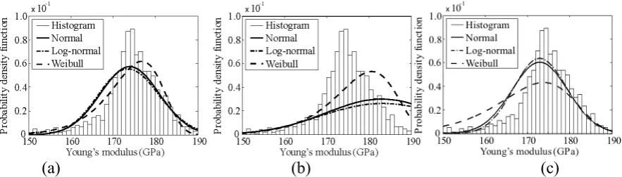
where is the mean and is the standard deviation, and t is a real variable.

119

- Log-normal distribution

120

2 2

ln

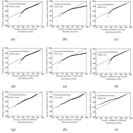
2 ₀

1

, 0,

PDF: ( | , ) ,

2

x

f e

x x

x , (3)

121

2

1 ln 2 0

1 1

CDF: ( | , ) .

2

t x

F x e dt

t (4)

122

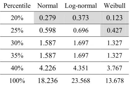
- Weibull distribution

123

Since previous studies [29] showed that the statistical characterisation of the CFRP does not 124

improve using a three-parameter Weibull distribution, a two-parameter approach was adopted here. 125

This is defined by the following expressions: 126

1

PDF: ( | , ) , , 0,0

x x

f x e x , (5)

127

CDF: ( | , ) 1 ,

x

F x e (6)

128

7

The best-fit distributions were found following the censored maximum likelihood estimation 130

(MLE) [30]. This method allows estimating parameters of a statistical distribution for a sample, 131

considering the following: 132

1 2

1

ˆ ˆ ˆ ˆ

( | , , , )_n n _X( | ),_i

i

L x x x f x (7)

133

in which L(.) is the likelihood that the parameters 1, , ,2 n properly describe the sample

134

1 2 ˆ ˆ ˆ, , ,ˆ_n

x x x x , and fX is the joint PDF of a sample. The maximum likelihood estimators are

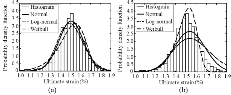
135

computed from the set of parameters that maximise the likelihood function by considering all 136

possible cases of . 137

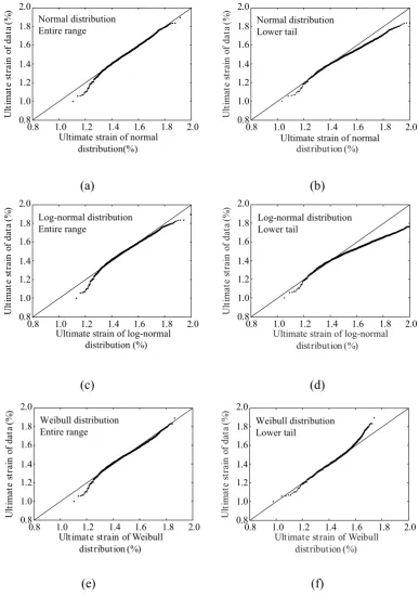
Since the tail region is critical for structural reliability analysis and prediction, especial attention 138

is given to this region in the statistical analysis of the tensile tests. The adopted technique considers 139

explicitly the values of the lower tail that are smaller than a predefined bound, whereas the 140

remaining values are used implicitly [31]. The censored MLE can be defined as follows: 141

1 2

L L L , (8)

142

with 143

1

1 ( | )

j

i i

L f x , (9)

144

2 ( | )n j

G

L P X x , (10)

145

( _G| ) 1 ( _G| )

P X x F x , (11)

146

where 1L is the likelihood associated with the j observations of values equal or lower than the 147

bound value x_G. 2L is the likelihood associated with the observations of values higher than the 148

bound value x_G. F x( G| ) is the CDF of xG given the PDF , n is the total number of

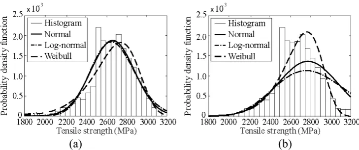
8

observations and n j is the total number of observations exceeding the bound value x_G. The best 150

fit can be computed iteratively through the optimisation problem of maximising L. 151

For each property, the distributions families were adjusted for the entire sample and the lower 152

percentiles of: 20th, 25th, 30th, 35th and 40th. The 20th percentile is considered to be a reasonable 153

choice for reliability studies in this research, since it includes the region of interest without 154

decreasing the sample size to statistically meaningless values. 155

The goodness of fit for all distributions was examined using the Anderson-Darling test for the: 156

(i) entire samples; and (ii) samples with right-censored data. The Anderson-Darling test was 157

adopted since it provides adequate comparison tools for tail regions [32]. The statistic for the right-158

censored data and entire data can be obtained respectively by [33]: 159

2

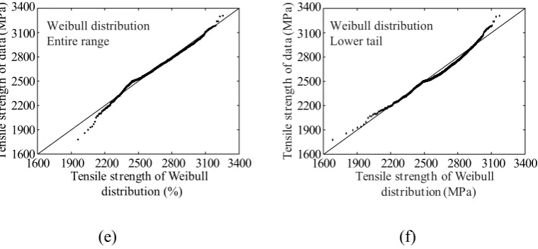
( ) ( 1 )

1

1 r _{(2 1) ln ln(1 )) ,}

i n i

i

A i Z Z n

n (12)

160

2 2 2 2

, ( ) ( ) ( ) ( ) ( ) ( )

1 1

1 1

(2 1) ln ln{1 } 2 ln{1 } ( ) ln{1 } ln ,

r r

r n i i i r r r

i i

A i Z Z Z r n Z r Z n

n n

161

(13) 162

where r is the uncensored observation, n is the total number of observations and Z denotes the 163

CDF of the probability distribution. The statistic values ( 2

A ) were then compared with the critical 164

values (CV) presented by Stephens and D'Agostino [33]. The null hypothesis (H0) of the data 165

following the distribution tests was not rejected if the statistic value was lower than the critical 166

value. The critical values for different percentiles are given in Table 2. To minimise Type I errors, 167

which occur when H0 was wrongly rejected, or Type II errors, in which H0 was wrongly accepted,

168

the significance level ( ) was set at 10%. 169

Table 2. Critical values for different percentiles. 170

Percentile 20% 25% 30% 35% 40% 100%

9

4.1. Young's modulus

171

The Young's modulus is one of the significant parameters related with the structural safety of the 172

FRP for rehabilitation of structures, particularly in situations where failure is expected to occur at 173

tensile stresses significantly lower than the ultimate strength of the FRP. This type of failure usually 174

occurs when debonding of the CFRP or concrete crushing are the dominant failure mechanisms [9]. 175

The best fit for each PDF for the Young's modulus is illustrated in Figure 3. As it can be seen in 176

Figure 3a, when the distributions were fitted to the entire sample, significant differences existed in 177

the range of the lower and upper values. Considering the importance of the tail regions in safety 178

assessment, clear improvements were achieved by applying the approach described above firstly to 179

the lower 20th percentile region – see Figure 3b. Both normal and log-normal distributions provided 180

similar results, whereas the Weibull distribution showed the closest fit to the data. For more clarity, 181

the Q-Q curves were plotted for three distributions in Figure 4. The Weibull distribution was able to 182

approximate the experimental data with high precision in both 20th percentile lower tail and entire 183

range regions (Figure 4e and Figure 4f). 184

185

(a) (b) (c)

186

Figure 3. PDF for the Young's modulus of: (a) the entire data fit, (b) the 20th percentile lower tail 187

fit; and (c) the 20th percentile upper tail fit. 188

10 190

(a) (b) (c)

191 192

193

(d) (e) (f)

194

195

(g) (h) (i)

196

Figure 4. Q-Q plot of the Young's modulus based on: normal distribution adjusted to (a) the 197

entire range, and (b) the 20th lower and (c) 20th upper percentile; log-normal distribution adjusted to 198

(d) the entire range, and (e) the 20th lower and (f) 20th upper percentile; and Weibull distribution 199

adjusted to (g) the entire range, and (h) the 20th lower and (i) 20th upper percentile. 200

The statistic values for the Anderson-Darling goodness of fit test are presented in Table 3. In this 201

table, the shaded cells refer to tests where the distributions were not rejected. The results showed 202

that the Weibull was the only distribution where the null hypothesis was not rejected for the highest 203

percentile (in this case the 25th). Additionally, this distribution presented the smallest statistical 204

130 140 150 160 170 180 190 200

100 120 140 160 200 180 Y ou ng ’ s m od ul us of da ta (G P a) distribution (GPa)

Young’s modulus of normal 130 140 150 160 170 180 190 200

100 120 140 160 180 200 Y ou ng ’ s m od ul us of da ta (G P a) distribution (GPa) Young’s modulus of normal Normal distribution

Entire range Normal distributionLower tail

130 140 150 160 170 180 190 200

100 120 140 160 200 180 Y ou ng ’ s m od ul us of da ta (G P a) distribution (GPa)

Young’s modulus of normal 130 140 150 160 170 180 190 200

100 120 140 160 180 200 Y ou ng ’ s m od ul us of da ta (G P a) distribution (GPa) Young’s modulus of normal Normal distribution

Entire range Normal distributionLower tail

Y ou ng ’ s m od ul us of da ta (G P a) distribution (GPa) Young’s modulus of normal

Y ou ng ’ s m od ul us of da ta (G P a)

Young’s modulus of log-normal distribution (GPa)

(a) (b)

130 140 150 160 170 180 190 200

100 120 140 160 200 180

130 140 150 160 170 180 190 200 100 120 140 160 180 200 Y ou ng ’ s m od ul us of da ta (G P a)

Young’s modulus of Weibull distribution (GPa)

130 140 150 160 170 180 190 200

100 120 140 160 200 180 (c) Normal distribution Upper tail Weibull distribution Upper tail Weibull distribution Upper tail

130 140 150 160 170 180 190 200

100 120 140 160 200 180 Y ou ng ’ s m od ul us of da ta (G P a)

Young’s modulus of log-normal distribution (GPa)

130 140 150 160 170 180 190 200 100 120 140 160 180 200 Y ou ng ’ s m od ul us of da ta (G P a)

Young’s modulus of log-normal distribution (GPa) Log-normal distribution

Entire range

Log-normal distribution Lower tail

130 140 150 160 170 180 190 200

100 120 140 160 200 180 Y ou ng ’ s m od ul us of da ta (G P a)

Young’s modulus of log-normal distribution (GPa)

130 140 150 160 170 180 190 200 100 120 140 160 180 200 Y ou ng ’ s m od ul us of da ta (G P a)

Young’s modulus of log-normal distribution (GPa) Log-normal distribution Entire range Log-normal distribution Lower tail Y ou ng ’ s m od ul us of da ta (G P a) distribution (GPa) Young’s modulus of normal

Y ou ng ’ s m od ul us of da ta (G P a)

Young’s modulus of log-normal distribution (GPa)

(a) (b)

130 140 150 160 170 180 190 200

100 120 140 160 200 180

130 140 150 160 170 180 190 200 100 120 140 160 180 200 Y ou ng ’ s m od ul us of da ta (G P a)

Young’s modulus of Weibull distribution (GPa)

130 140 150 160 170 180 190 200

100 120 140 160 200 180 (c) Weibull distribution Upper tail Log-normal distribution Upper tail Weibull distribution Upper tail

130 140 150 160 170 180 190 200 100 120 140 160 180 200 Y ou ng ’ s m od ul us of da ta (G P a) distribution (GPa)

Young’s modulus of Weibull 130 140 150 160 170 180 190 200

100 120 140 160 180 200 Y ou ng ’ s m od ul us of da ta (G P a) distribution (GPa) Young’s modulus of Weibull Weibull distribution

Entire range

Weibull distribution Lower tail

130 140 150 160 170 180 190 200 100 120 140 160 180 200 Y ou ng ’ s m od ul us of da ta (G P a) distribution (GPa)

Young’s modulus of Weibull 130 140 150 160 170 180 190 200

100 120 140 160 180 200 Y ou ng ’ s m od ul us of da ta (G P a) distribution (GPa) Young’s modulus of Weibull Weibull distribution Entire range Weibull distribution Lower tail Y ou ng ’ s m od ul us of da ta (G P a) distribution (GPa) Young’s modulus of normal

Y ou ng ’ s m od ul us of da ta (G P a)

Young’s modulus of log-normal distribution (GPa)

(a) (b)

130 140 150 160 170 180 190 200 100 120 140 160 200 180

130 140 150 160 170 180 190 200 100 120 140 160 180 200 Y ou ng ’ s m od ul us of da ta (G P a)

Young’s modulus of Weibull distribution (GPa)

11

values, meaning that the average squared distance between the data and the fitted distribution was 205

also the lowest. 206

Table 3. Statistical values for the Anderson-Darling goodness of fit test for each percentile and 207

distribution. 208

Percentile Normal Log-normal Weibull

20% 0.279 0.373 0.123

25% 0.598 0.696 0.427

30% 1.587 1.697 1.327

35% 1.587 1.697 1.327

40% 4.226 4.351 3.767

100% 18.236 23.568 13.678

209

Based on the statistical analysis of the experimental data, the following shape and scale 210

parameters were proposed to model the Young’s modulus based on the Weibull distribution 211

adjusted to the 20th percentile: 212

~ W(26.2,180.9) GPa. f

E (14)

213

Depending on the design situation, the upper percentile of the Young’s modulus might also be 214

required. For example, in situations of debonding failure, an higher value for this material 215

parameter can provide more conservative estimates on the capacity of the structural member. For 216

this reason, the study described in this section was similarly applied to obtain the best fit 217

distribution for the 20th upper percentile. Results are shown in Figs. 3 and 4, whereas the Weibull 218

distribution adjusted to the upper tail region was given by the following equation: 219

~ W(20.4,174.4) GPa. f

E (15)

220

Using the distributions shown in Eqs. (14) and (15), the characteristic values for the Young's 221

modulus were determined as 161.5 GPa and 184.0GPa, respectively corresponding to the 5th and 222

12

value provided by the manufacturer (165 GPa). Results also showed that the coefficient of variation 224

was reduced, i.e., 0.04. 225

4.2. Ultimate strain

226

The ultimate strain of the FRP is another important parameter in structural safety since the 227

material typically exhibits elastic behaviour until failure. The same procedure described above was 228

followed to analyse this material parameter from the tensile tests. Conversely to what was observed 229

for the Young’s modulus, the statistical analysis showed that (Figure 5a) none of the selected 230

distributions could fit well the lower tail when using the entire sample. Figure 5b shows the ultimate 231

strain probability density functions adjusted to the lower tail, where the Weibull distribution was the 232

one that provided the best results. The same trend could be seen in the corresponding Q-Q plots 233

illustrated in Figure 6. 234

235

(a) (b)

236

Figure 5. PDF for the ultimate strain of the entire data fit (a) and 20th percentile lower tail fit (b). 237

The Anderson-Darling goodness of fit test presented in Table 4 shows that the Weibull was the 238

only distribution not rejected for the highest percentile (in this case the 40th), whereas the null 239

hypothesis was rejected for all the distributions adjusted to the entire sample. Based on these 240

results, the Weibull distribution adjusted to the 20th percentile was proposed to model the ultimate 241

strain with a coefficient of variation of 0.06, and the following parameters: 242

~ W(17.1,1.5) %.

fu (16)

13 244

(a) (b)

245

246

(c) (d)

247

248

(e) (f)

249

Figure 6. Q-Q plot of the ultimate strain based on: normal distribution adjusted to (a) the entire 250

range and (b) the lower tail; log-normal distribution adjusted to (c) the entire range and (d) the 20th 251

lower percentile; and Weibull distribution adjusted to (e) the entire range and (f) the 20th lower 252

percentile. 253

254

1.0

0.8 1.2 1.4 1.6 1.8 2.0

1.0 0.8 1.2 1.4 1.6 1.8 2.0 distribution(%) U lt im at e st ra in of da ta (% )

Ultimate strain of normal 0.8 1.0 1.2 1.4 1.6 1.8 2.0

1.0 0.8 1.2 1.4 1.6 1.8 2.0 distribution (%) U lt im at e st ra in of da ta (% )

Ultimate strain of normal Normal distribution

Entire range Normal distributionLower tail

1.0

0.8 1.2 1.4 1.6 1.8 2.0

1.0 0.8 1.2 1.4 1.6 1.8 2.0 distribution(%) U lt im at e st ra in of da ta (% )

Ultimate strain of normal 0.8 1.0 1.2 1.4 1.6 1.8 2.0

1.0 0.8 1.2 1.4 1.6 1.8 2.0 distribution (%) U lt im at e st ra in of da ta (% )

Ultimate strain of normal Normal distribution

Entire range Normal distributionLower tail

1.0

0.8 1.2 1.4 1.6 1.8 2.0

1.0 0.8 1.2 1.4 1.6 1.8 2.0

Ultimate strain of log-normal

U lt im at e st ra in of da ta (% ) distribution (%) 1.0

0.8 1.2 1.4 1.6 1.8 2.0

1.0 0.8 1.2 1.4 1.6 1.8 2.0 distribution (%) U lt im at e st ra in of da ta (% )

Ultimate strain of log-normal

Log-normal distribution Entire range

Log-normal distribution Lower tail

1.0

0.8 1.2 1.4 1.6 1.8 2.0

1.0 0.8 1.2 1.4 1.6 1.8 2.0

Ultimate strain of log-normal

U lt im at e st ra in of da ta (% ) distribution (%) 1.0

0.8 1.2 1.4 1.6 1.8 2.0

1.0 0.8 1.2 1.4 1.6 1.8 2.0 distribution (%) U lt im at e st ra in of da ta (% )

Ultimate strain of log-normal

Log-normal distribution Entire range

Log-normal distribution Lower tail

1.0

0.8 1.2 1.4 1.6 1.8 2.0

1.0 0.8 1.2 1.4 1.6 1.8 2.0 distribution (%) Ultimate strain of Weibull

U lt im at e st ra in of da ta (% ) 1.0

0.8 1.2 1.4 1.6 1.8 2.0

1.0 0.8 1.2 1.4 1.6 1.8 2.0 distribution (%) Ultimate strain of Weibull

U lt im at e st ra in of da ta (% ) Weibull distribution

Entire range Weibull distributionLower tail

1.0

0.8 1.2 1.4 1.6 1.8 2.0

1.0 0.8 1.2 1.4 1.6 1.8 2.0 distribution (%) Ultimate strain of Weibull

U lt im at e st ra in of da ta (% ) 1.0

0.8 1.2 1.4 1.6 1.8 2.0

1.0 0.8 1.2 1.4 1.6 1.8 2.0 distribution (%) Ultimate strain of Weibull

U lt im at e st ra in of da ta (% ) Weibull distribution

14

Table 4. Statistical values for the Anderson-Darling goodness of fit test for each percentile and 255

distribution. 256

Percentile Normal Log-normal Weibull

20% 0.206 0.351 0.050

25% 0.237 0.393 0.057

30% 0.433 0.656 0.101

35% 0.771 1.148 0.126

40% 1.371 2.056 0.136

100% 2.5453 5.485 8.9873

4.3. Tensile strength

257

The tensile strength of the FRP is important in situations where failure occurs within the 258

laminate. This can be particularly critical for prestressed FRP laminates, since the prestress loading 259

often represents a high percentage of the tensile strength [34, 35]. Preliminary results of the 260

distributions adjusted to the entire sample showed that all selected distributions were unable to 261

provide a good fit in the lower tail, as illustrated in Figure 7a. An improvement could be obtained 262

when the procedure based on fitting the CDF to the lower tail is followed – see Figure 7b. The 263

Weibull distribution performed better in both cases. 264

265

(a) (b)

266

Figure 7. PDF for the tensile strength of (a) the entire data fit (b) and the 20th percentile lower tail 267

fit. 268

The Q-Q plots showed the similarity between normal and log-normal distributions – see 269

15

fit obtained with the Weibull distribution in this region can be noticed by comparing Figure 8e and 271

f. Despite these observations, the goodness of fit results for the lowest tail fit (Table 5) did not reject 272

any of the distributions for the 20th and 25th percentiles. However, since the Weibull presented a 273

better result than the other models overall, it was adopted here as the distribution model for the 274

tensile strength with the following parameters: 275

~ W(15.9, 2777.0) MPa. f

f (17)

276

The 5th characteristic value using the proposed distribution was 2304.2 MPa, which was only 277

0.3% higher than the experimental value (2299.0 MPa). The coefficient of variation was also very 278

small, i.e. 0.08. The selected distribution is in agreement with the works from Atadero [23] and 279

Zureick, Bennett [24] for prediction of the tensile strength based on the entire data fit. 280

281

(a) (b)

282

283

(c) (d)

284

1600 1900 2200 2500 2800 3100 3400 1600 1900 2200 2800 3100 2500 3400 distribution (MPa) Tensile strength of Normal

T en si le st re ng th of da ta (M P a)

1600 1900 2200 2500 2800 3100 3400 1600 1900 2200 2800 3100 2500 3400 distribution (MPa) Tensile strength of Normal

T en si le st re ng th of da ta (M P a) Normal distribution

Entire range Normal distribution_{Lower tail}

1600 1900 2200 2500 2800 3100 3400 1600 1900 2200 2800 3100 2500 3400 distribution (MPa) Tensile strength of Normal

T en si le st re ng th of da ta (M P a)

1600 1900 2200 2500 2800 3100 3400 1600 1900 2200 2800 3100 2500 3400 distribution (MPa) Tensile strength of Normal

T en si le st re ng th of da ta (M P a) Normal distribution

Entire range Normal distribution_{Lower tail}

1600 1900 2200 2500 2800 3100 3400 1600 1900 2200 2800 3100 2500 3400

Tensile strength of Log-normal

T en si le st re ng th of da ta (M P a) distribution (MPa)

1600 1900 2200 2500 2800 3100 3400 1600 1900 2200 2800 3100 2500 3400 T en si le st re ng th of da ta (M P a)

Tensile strength of Log-normal distribution (MPa) Log-normal distribution

Entire range

Log-normal distribution Lower tail

1600 1900 2200 2500 2800 3100 3400 1600 1900 2200 2800 3100 2500 3400

Tensile strength of Log-normal

T en si le st re ng th of da ta (M P a) distribution (MPa)

1600 1900 2200 2500 2800 3100 3400 1600 1900 2200 2800 3100 2500 3400 T en si le st re ng th of da ta (M P a)

Tensile strength of Log-normal distribution (MPa) Log-normal distribution

Entire range

16 285

(e) (f)

286

Figure 8. Q-Q plot of the tensile strength based on: normal distribution adjusted to (a) the entire 287

range and (b) the lower tail; log-normal distribution adjusted to (c) the entire range and (d) the 20th 288

lower percentile; and Weibull distribution adjusted to (e) the entire range and (f) the 20th lower 289

percentile. 290

Table 5. Statistical values for the Anderson-Darling goodness of fit test for each percentile and 291

distribution. 292

Percentile Normal Log-normal Weibull

20% 0.050 0.068 0.064

25% 0.342 0.366 0.333

30% 0.894 0.941 0.817

35% 2.518 2.658 2.154

40% 4.160 4.429 3.404

100% 5.453 5.485 9.897

5. Correlation Analysis

293

This section presents a correlation analysis on the mechanical properties discussed in the 294

previous section. Within the linear elastic range, strain, stress and Young’s modulus are naturally

295

related with each other by the Hooke’s law. When approaching ultimate values – i.e. the material 296

strength – the standard relation may no longer hold and more suitable relationships may need to be 297

recommended for reliability analysis. The following pairs were considered: (i) tensile strength and 298

1600 1900 2200 2500 2800 3100 3400 1600

1900 2200 2800 3100

2500 3400

Tensile strength of Weibull

T

en

si

le

st

re

ng

th

of

da

ta

(M

P

a)

distribution (%)

1600 1900 2200 2500 2800 3100 3400 1600

1900 2200 2800 3100

2500 3400

T

en

si

le

st

re

ng

th

of

da

ta

(M

P

a)

distribution (MPa) Tensile strength of Weibull Weibull distribution

Entire range

Weibull distribution Lower tail

1600 1900 2200 2500 2800 3100 3400 1600

1900 2200 2800 3100

2500 3400

Tensile strength of Weibull

T

en

si

le

st

re

ng

th

of

da

ta

(M

P

a)

distribution (%)

1600 1900 2200 2500 2800 3100 3400 1600

1900 2200 2800 3100

2500 3400

T

en

si

le

st

re

ng

th

of

da

ta

(M

P

a)

distribution (MPa) Tensile strength of Weibull Weibull distribution

Entire range

17

ultimate strain, (ii) tensile strength and Young's modulus, and (iii) Young's modulus and ultimate 299

strain. 300

A linear regression analysis was firstly performed between tensile strength and ultimate strain 301

without constraints. Results showed high correlation between these two properties (R2 = 0.75) as

302

illustrated in Figure 9a. Additionally, the residual standard deviation related with the uncertainty of 303

the proposed model was 0.062%, which means that a probabilistic model could indeed describe the 304

correlation between the two mechanical parameters. The corresponding model was defined as 305

follows: 306

0.17 0.0005014 0.0618 (%),

fu ff Z (18)

307

where f_f is the tensile strength in MPa, _fu is the ultimate strain and Z ~ (0,1)N . 308

Based on the results above, a second correlation analysis was performed by constraining the 309

linear relation to the origin. The results and observations were quite similar, as shown in Figure 9b. 310

The latter model had a standard deviation of 0.063% and was defined by the following expression: 311

0.0005646 0.0633 (%)

fu ff Z . (19)

312

The last expression can be recommended in practice to relate the two expressions, since it provides 313

good results and is relatively simple. It should be mentioned that such result shows that the ultimate 314

strain and tensile strength are highly correlated variables. However, since both are not deterministic, 315

the numerical value in the equation should not be directly compared with the inverse ratio of the 316

Young’s modulus – although both are similar given the linear nature of the correlation found. 317

It should be highlighted that from this study, the tensile strength and Young's modulus were 318

found to have a small correlation – see representation in Figure 10a. Similar observation was also 319

found between the Young's modulus and ultimate strain (Figure 10b). This suggests that the 320

18 322

(a) (b)

323

Figure 9. Scatter diagram of tensile strength versus ultimate strain of (a) the regression without 324

constraints and (b) the regression across the origin. 325

326

(a) (b)

327

Figure 10. Scatter diagram of (a) tensile strength versus Young's modulus ( f_f , Ef ) and (b) 328

Young's modulus versus ultimate strain (E_f , _fu). 329

6. Conclusions

330

This manuscript presented a statistical analysis on mechanical properties of prefabricated CFRP 331

laminates obtained from a large set of tests. Results showed that the Weibull distribution can be 332

adopted to model the Young's modulus, the ultimate strain and the tensile strength of CFRP 333

19

carried out giving particular attention to the tail region. In fact, although an overall good fit of any 335

selected distribution can be achieved in most cases, the approximation obtained in the tail region is 336

not acceptable. 337

A low variability in the mechanical properties was also observed in this study, which is most 338

significant in terms of structural safety. The lowest coefficient of variation is found for the Young's 339

modulus, with the characteristic values from experimental data and proposed distributions being 340

also very similar. 341

The correlation analysis between mechanical properties demonstrated that a probabilistic model 342

relating the tensile strength and ultimate strain can be proposed. However, despite the strain, stress 343

and Young’s modulus being related by the Hooke’s law in the linear elastic region, no probabilistic 344

model could be proposed between tensile strength or ultimate strain and Young's modulus. In fact, 345

these pairs of variables can be considered as independent. 346

As a final note, it should be mentioned that the distributions given in this paper can be used for 347

carrying out reliability analyses aimed at proposing partial safety factors for the future revision of 348

design codes. 349

Acknowledgements

350

The authors acknowledge the experimental tests data provided by S&P Clever Reinforcement 351

Ibérica. Sara Gomes would like to acknowledge the research grant from the Portuguese Science and 352

Technology Foundation (SFRH/BD/76345/2011) and D. Dias-da-Costa would like to acknowledge 353

the support from the Australian Research Council through its Discovery Early Career Researcher 354

Award (DE 150101703) and from the Faculty of Engineering and Information Technologies, The 355

20

Appendix A: sample distribution

357

Table A-1 provides the sample size and geometrical data for the 1368 coupon samples studied in 358

this paper. 359

Table A-1. Details of coupon samples. 360

Cross-section

(mm2_{) (mm}Area 2₎ Sample size _(#)

50 1.2 60 85

50 1.4 70 422

60 1.4 8.4 54

80 1.2 96 110

80 1.4 112 122

90 1.4 126 41

100 1.2 120 144

100 1.4 140 192

120 1.2 144 43

120 1.4 168 155

References

361

[1] Leeming MB, Hollaway LC. Strengthening of reinforced concrete structures: Woodhead Publishing 362

Limited; 1999. 363

[2] Hadigheh SA, Gravina RJ, Setunge S. Influence of the processing techniques on the bond characteristics 364

in externally bonded joints- Experimental and analytical investigations. Composites for Construction. 365

2016;20:1-13. 366

[3] Hadigheh SA, Gravina RJ. Generalization of the interface law for different FRP processing techniques in 367

FRP-to-concrete bonded interfaces. Composites Part B: Engineering. 2016;91:399-407. 368

[4] Karbhari VM. Materials considerations in FRP rehabilitation of concrete structures. Journal of Materials 369

in Civil Engineering. 2001;13:90-7. 370

[5] Mirmiran A, Shahawy M, Samaan M, Echary HE, Mastrapa JC, Pico O. Effect of column parameters on 371

FRP-confined concrete. Journal of Composites for Construction. 1998;2:175-85. 372

[6] Khalifa A, Gold WJ, Nanni A, Abdel Aziz MI. Contribution of externally bonded FRP to shear capacity 373

of RC flexural members. Journal of Composites for Construction. 1998;2:195-202. 374

[7] Hadigheh SA, Gravina RJ, Setunge S. Prediction of the bond-slip law in externally laminated concrete 375

substrates by an analytical based nonlinear approach. Materials and Design. 2015;66:217-26. 376

[8] Smith ST, Zhang H, Wang Z. Influence of FRP anchors on the strength and ductility of FRP-strengthened 377

RC slabs. Constr Build Mater. 2013;49:998-1012. 378

[9] CEB-FIB. FIB-Bulletin 14- Externally bonded FRP reinforcement for RC structures. Geneva, 379

Switzerland: Fédération International du Béton (FIB); 2001. p. 130. 380

[10] TR-55. Design guidance for strenghening concrete structures using fibre composite materials. 381

SOCIETY, C.(ed.); 2000. 382

[11] CNR. Guide for the design and construction of externally bonded FRP systems for strengthening 383

existing structures. National Research Council, Advisory Committee on Technical Recommendations for 384

Constructuion2001. 385

[12] ACI 440.2R-08. Guide for the design and construction of externally bonded FRP system for 386

21

[13] Ellingwood BR. Toward load and resistance factor design for fiber-reinforced polymer composite 388

structures. Journal of Structural Engineering. 2003;129:449-58. 389

[14] Wang N, Ellingwood BR, Zureick AH. Reliability-based evaluation of flexural members strengthened 390

with externally bonded fiber-reinforced polymer composites. Journal of Structural Engineering. 391

2010;136:1151-60. 392

[15] Plevris N, Triantafillou TC, Veneziano D. Reliability of RC members strengthened with CFRP 393

laminates. Journal of Structural Engineering. 1995;121:1037-44. 394

[16] Okeil AM, El-Tawil S, Shahawy M. Flexural reliability of reinforced concrete bridge girders 395

strengthened with carbon fiber-reinforced polymer laminates. Journal of Bridge Engineering. 2002;7:290-9. 396

[17] Monti G, Santini S. Reliability-based calibration of partial safety coefficients for fiber-reinforced 397

plastic. Journal of Composites for Construction. 2002;6:162-7. 398

[18] Atadero R, Lee L, Karbhari VM. Consideration of material variability in reliability analysis of FRP 399

strengthened bridge decks. Composite Structures. 2005;70:430-43. 400

[19] Atadero RA, Karbhari VM. Calibration of resistance factors for reliability based design of externally-401

bonded FRP composites. Composites Part B: Engineering. 2008;39:665-79. 402

[20] Okeil AM, Belarbi A, Kuchma DA. Reliability assessment of FRP-strengthened concrete bridge girders 403

in shear. Journal of Composites for Construction. 2013;17:91-100. 404

[21] Ali O, Bigaud D, Ferrier E. Comparative durability analysis of CFRP-strengthened RC highway 405

bridges. Constr Build Mater. 2012;30:629-42. 406

[22] Atadero RA, Karbhari VM. Sources of uncertainty and design values for field-manufactured FRP. 407

Composite Structures. 2009;89:83-93. 408

[23] Atadero RA. Development of load and resistance factor design for FRP strengthening of reinforced 409

concrete structures: PhD Thesis, University of California; 2006. 410

[24] Zureick AH, Bennett RM, Ellingwood BR. Statistical characterization of fiber-reinforced polymer 411

composite material properties for structural design. Journal of Structural Engineering. 2006;132:1320-7. 412

[25] Jeong HK, Shenoi RA. Probabilistic strength analysis of rectangular FRP plates using Monte Carlo 413

simulation. Computers & Structures. 2000;76:219-35. 414

[26] Lekou DJ, Philippidis TP. Mechanical property variability in FRP laminates and its effect on failure 415

prediction. Composites Part B: Engineering. 2008;39:1247-56. 416

[27] Ellingwood BR. Acceptable risk bases for design of structures. Progress in Structural Engineering and 417

Materials. 2001;3:170-9. 418

[28] EN ISO 527-5. Plastics- Determination of tensile properties, Part 5: Test conditions for unidirectional 419

fibre-reinforced plastic composites. European Committee for Standardization; 2009. 420

[29] Alqam M, Bennett RM, Zureick AH. Three-parameter vs. two-parameter Weibull distribution for 421

pultruded composite material properties. Composite Structures. 2002;58:497-503. 422

[30] Lindley DV. Introduction to probability and statistics. Cambridge University Press1965. 423

[31] Havbro Faber M, Köhler J, Dalsgaard Sorensen J. Probabilistic modeling of graded timber material 424

properties. Structural Safety. 2004;26:295-309. 425

[32] Lawless JF. Statistical models and methods for lifetime data: Wiley; 1982. 426

[33] Stephens M, D'Agostino R. Goodness-of-fit techniques: Marcel Dekker; 1986. 427

[34] Quantrill RJ, Hollaway LC. The flexural rehabilitation of reinforced concrete beams by the use of 428

prestressed advanced composite plates. Composites Science and Technology. 1998;58:1259-75. 429

[35] Triantafillou TC, Deskovic N, Deuring M. Strengthening of concrete structures With prestressed fiber 430

reinforced plastic sheets. Structural Journal. 1992;89:235-44. 431