J. Phys. A: Math. Theor.40(2007) 65–74 doi:10.1088/1751-8113/40/1/004
Topological events on wave dislocation lines: birth and
death of loops, and reconnection
M V Berry1and M R Dennis2
1H H Wills Physics Laboratory, Tyndall Avenue, Bristol BS8 1TL, UK
2School of Mathematics, University of Southampton, Highfield, Southampton SO17 1BJ, UK
Received 6 October 2006 Published 6 December 2006
Online atstacks.iop.org/JPhysA/40/65
Abstract
In three-dimensional space, a wave dislocation, that is, a quantized (optical) vortex or phase singularity, is a line zero of a complex scalar wavefunction. As a ‘time’ parameter varies, the topology of the vortex can change by encounter with a line of vanishing vorticity (curl of the current associated with the wavefunction). An isolated critical point of the field intensity, sliding along the zero-vorticity line like a bead on a wire, meets the vortex as it encounters the line, and so participates in the singular event. Local expansion and gauge and coordinate transformations show that the vortex topology can change generically by the appearance or disappearance of a loop, or by the reconnection of branches of a pair of hyperbolas.
PACS numbers: 02.40.Xx, 03.65.Vf, 03.75.Lm, 42.25.Fx, 67.40.Vs
1. Introduction
Lines of phase singularity are important morphological elements of complex scalar fields. When the field represents a wave (for example a linearly polarized optical field), phase singularities are also known as wave dislocations, wave (or optical) vortices, and nodal lines. They have been studied extensively, both theoretically and experimentally [1–4]. In quantum waves, they are also referred to as quantized vortex lines, and have important physical consequences [5,6]. Unlike their counterparts in fluid mechanics, the location of these wave vortices is determined purely by the vanishing of the complex wavefunction, so that wave vortices are places where the phase is undefined. In three-dimensional space, the vortex lines display a variety of geometries, and can be curved, linked or knotted [7–10], in ways at most only weakly constrained by equations (linear or not) that the waves satisfy.
Here we will investigate phase singularity lines in three-dimensional space, whose geometry depends on a parameter that we will call ‘time’. Our aim is to establish the generic (that is, structurally stable) events in which phase singularities in space can meet and change their topology, or spontaneously appear and disappear. Some of our conclusions have appeared
in previous studies of controlled creation and reconnection events in optical vortices [11,12], associated with knots, links and braids [8,13], and the development of diffraction catastrophes [14] and other three-dimensional situations where a parameter varies [15,16]. Reconnections have also been studied for vortices in superfluids [17], in the Schr¨odinger equation (both linear [18] and nonlinear [19]), and in cosmic strings [20]. However, the subject deserves a closer look, because general statements and formulas, as well as a connection we uncover between phase and intensity singularities, have been lacking.
The fact that vortices are lines follows from a familiar codimension argument: as nodal lines in the complex wavefield, they occur on the lines of intersection of the zero contour surfaces of the real and imaginary parts of the field (i.e. the vortices have codimension 2). The events we study here, in which the vortices change topology, have codimension 4—two to be at a node (zero surfaces intersect), and two more so that the tangent planes to the zero surfaces are parallel, so the surfaces touch. The details will be described in section3.
Here we will be studying topological changes of vortex lines in three dimensions. Interactions between vortex points in the plane are much simpler: generically, points can appear or annihilate in pairs of opposite strength, these events occurring in the presence of phase saddles [21]. If the plane being considered is an observation screen {x, y}in three-dimensional space {x, y, z}(for example in paraxial optics), interactions of points on the screen aszvaries can give the illusion of a three-dimensional interaction, when all that is really happening is a tangency between the screen and a smoothly curved vortex line in space [22].
2. Participating singularities
Let the wavesψthat we will consider, expressed in terms of their modulus, phase, and real and imaginary parts, be written as
ψ(r, t )=ρ(r, t )exp{iχ (r, t )} =ξ(r, t )+ iη(r, t ) (r= {x, y, z}). (1) The vortices, which have codimension 2 and so are lines in space, satisfy
vortex lines: ψ=0 ⇒ ξ =η=0. (2)
They are quantized: in a loop around the vortex line, the phase changes by 2π (quantized vortices of higher strength have a higher codimension, and are not considered here). Associated with the phase are two vectors. First is the currentj, whose streamlines (orthogonal to the wavefrontsχ=constant) wind around the vortices [23,24]:
j=Imψ∗∇ψ=ρ2∇χ . (3) Second is the vorticity
Ω=1
2∇ ×j= 1
2Im(∇ψ∗× ∇ψ )= ∇ξ× ∇η. (4) This vector exists everywhere, and in particular on a vortex line, whose tangent atris parallel toΩ(r) (because vortices are intersections of the surfacesξ =0,η=0).
Loci of vanishingΩ(irrotational lines) play an important role in the life of a vortex line, because ifΩ=0 on a vortex line, its tangent direction is undefined. The loci are
Ω=0,i.e.∇ξ and∇ηparallel(or antiparallel). (5) Thus whereΩ=0 the complex vector∇ψis a real vector (in the common direction of∇ξ
and∇η) multiplied by a phase factor. The loci are lines, notwithstanding the three conditions corresponding to each component ofΩ, because these are not independent: from (4),Ω=
a codimension 2 requirement. Usually theΩ =0 lines and the vortices are distinct, but, as is intuitively plausible and will be shown in the next section, encounter is possible as time varies. We will show that at such events (codimension 4 in total), the topology of the vortex line changes, in one of two possible ways.
First we note a connection, important in what follows, between singularities of phase and the intensity
I = |ψ|2=ρ2. (6)
Consider the loci of vanishing∇I. These fall into two classes. First are the vortices: lines (codimension 2) whereρvanishes, across whichρ2has a smooth minimum. In addition, there are points (codimension 3) whereIdoes not vanish:
intensity critical points :
isolated points where∇I =0, i.e. ξ∇ξ +η∇η=0 andI =0. (7)
At intensity critical points,∇ξ and∇ηmust be parallel or antiparallel, so these points lie on theΩ=0 lines. Over time, the intensity critical points move along theΩ=0 lines like beads sliding on a wire, and theΩ =0 lines themselves can move. In the next section, we will show that as a vortex meets anΩ=0 line at a topology-changing event, an isolated intensity critical point participates in the encounter by arriving at the same instant.
It is not hard to confirm that vortex lines and isolated intensity critical points are invariant under arbitrary gauge transformations (multiplication by a smooth, possibly coordinate- and time-dependent phase factor, that is, a rotation in theξ,ηplane), and arbitrary smooth linear or nonlinear coordinate transformations. TheΩ=0 lines, on the other hand, generally deform under a gauge transformation, though they are pinned at the isolated intensity critical points. (If a constant is added toψ, the vortices and intensity critical points move, but theΩ=0 lines do not; this property was used [8] to tune reconnections in knotting vortices.)
3. Neighbourhood of the topology-changing events
Consider anΩ=0 line passing through the origin at some instant, so that∇ξ and∇ηare parallel. If a vortex line passes though the origin at the same time,ψmust have the local form
ψ=a·r+12r·A·r+· · · (8)
whereais a vector whose real and imaginary parts are parallel (i.e. ais a real vector times a phase factor, soa∗×a=0), andAis a complex 3×3 symmetric matrix. At small non-zero times, the vortex and theΩ =0 line will typically no longer coincide, and neither will pass through the origin. However, by choosing a moving coordinate frame theΩ=0 line can be made to continue to pass through the origin. Butψwill no longer vanish atr=0.
At first it seems as though a complex ‘time’ parameter,τ say, is required to unfold the singularity, that is
ψ=τ +a·r+21r·A·r+· · ·. (9)
This would correspond to the two real parameters Reτ and Imτ. Nevertheless, we now show that the events we are considering have real codimension 4: space (r) plus just one real time parameter. Referring to figure1, we consider values ofψ at points on theΩ =0 line, in the complexξ,ηplane. When theΩ=0 line intersects a dislocation line at the coordinate origin, its image in theψplane crosses O. For times close to this intersection, there will be a point P closest to O, where it is obvious thatI = |ψ|2=ξ2+η2is stationary with respect to displacements along theΩ=0 line, that is
O S
P
complex plane
=0
Figure 1.Complexψplane for a time near a topology-changing event. The origin O corresponds to the dislocation, the thick curve is the image of theΩ=0 line (5), on which lie the point P corresponding to an isolated intensity critical point (7), and the cusp point S (irrelevant to the topology-changing event) corresponding to a place where theΩ=0 line is perpendicular to the common direction of∇ξand∇η.
wheredis the direction of theΩ=0 line, andeandcare defined by
∇η=c∇ξ =c|∇ξ|e. (11)
The condition (10) corresponding to P can be satisfied either by∇I = 0 (i.e. ξ + cη=0) or byd·e=0. We ignore points S whered·e=0, because when∇ξ and∇ηare perpendicular to the direction of theΩ=0 line neitherξnorηis changing, and S corresponds to a special (cusp) point, unrelated to O, requiring two parameters to encounter O (we will return to thed·e =0 points later). On the other hand, one parameter suffices to make the image curve encounter O, so at the corresponding P, where the curve is smooth, we must have
ξ + cη=0. This implies the vanishing of all components of∇I, not just the component along theΩ=0 line. Thus we have justified the assertion that an isolated critical point must participate in the topology-changing event.
It is convenient to chooseτ real in a gauge whereais imaginary, and orient coordinate axes such thatapoints in thezdirection. Thus without loss of generality (9) can be replaced by
ψ=t+ iaz+ 12r·A·r+· · ·, (12)
wheretandaare real and againAis a complex 3×3 symmetric matrix.
The vortex lines at timetare conveniently determined by separating the components ofr
perpendicular and parallel toa, so
t+ 12R·(ReA⊥)·R+zReb·R+ 12z2ReA33=0
(13)
az+12R·(ImA⊥)·R+zImb·R+ 12z2ImA33 =0, where
r= {R, z}, R= {x, y}, A⊥=
A11 A12
A12 A22
, b= {A13, A23}. (14)
From the second equation in (13), representing theη=0 surface, the vortices lie on the fixed surface with height
z= −R·(ImA⊥)·R
2a +· · ·, (15)
where . . . represents terms cubic and higher inR. The first equation in (13), representing the
ξ =0 surface, gives the projection of the vortices onto the planez=0:
0 1 -1 -1 -1 0 1 0 1 0 1 0 1
(a)
x y z i ii iii 0 0.5 -0.5 0 0.5 -0.3 0 0.3 -0.5 0 0 5
(b)
[image:5.595.158.466.93.253.2]x y z i i ii ii iii iii iv iv
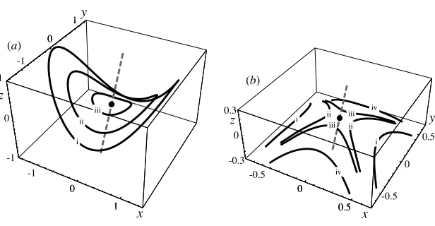
Figure 2.Topology-changing events. (a) Vortex loop shrinking and vanishing, for (A11=1−i, A22=2 + i,A12=A13=0,A23= −1,A33arbitrary) and times i: t= −1; ii: t= −0.5; iii: t= −0.1; dashes denote theΩ=0 line, and the black dot is the isolated intensity critical point. (b) As (a), for (A11=1 + i,A22= −1 + i,A12=A13=0,A23=0.5,A33arbitrary) and times i: t= −0.1; ii:t= −0.01; iii:t=+0.01; iv:t=+0.1.
In the gauge corresponding to (12), the vortex geometry is determined by the gaussian curvature of theξ =0 surface, that is by det ReA⊥. If det ReA⊥ >0, (16) represents an elliptical vortex loop shrinking to a point and vanishing ast→0 from below/above, if the eigenvalues of ReA⊥are both positive/negative. If det ReA⊥ <0, (16) represents a pair of hyperbolas whose branches reconnect att=0, when they degenerate into a cross. These are the two stable possibilities for vortex topology change, illustrated in figure2.
Equation (14) shows that in general the vortex is not planar, but flattens near the singularity. Using polar coordinatesR= {R, φ}, we can combine (15) and (16) into
az
t =
ImA11cos2φ+ 2 ImA12sinφcosφ+ ImA22sin2φ ReA11cos2φ+ 2 ReA12sinφcosφ+ ReA22sin2φ
=tan argR·A⊥·R, (17)
showing that each point on the vortex approaches theRplane at a constant speed, which in the hyperbolic case is infinitely fast at the asymptotes.
From
∇ξ =ReA·r, ∇η=aez+ ImA·r, (18)
it follows that the local form of theΩ=0 line, where∇ξ and∇ηare parallel, is determined by
(aez+ ImA·r)×ReA·r=0. (19)
In the appendix we give the general solution of this equation, and show that near the origin the form of theΩ=0 line, parameterized byz, is
R(z)=z
(ReA)−1 ·ez
⊥
ez·(ReA)−1 ·ez = −z
ReA13 ReA11
, ReA23
ReA22
, (20)
The single intensity critical point determined by (7) is fixed at the origin r=0. This follows directly from (12), which shows that whent=0 the intensity|ψ|2 has a quadratic critical point atr=0; as previously argued, at the instantt =0 of the singular event, the vortex collides with the critical point, which becomes degenerate (locally cubic).
The general picture we have derived is of a vortex loop shrinking onto an isolated intensity critical point on anΩ =0 line, or two vortex lines crossing at an isolated intensity critical point on anΩ=0 line. Particular waves displaying both types of behaviour have been found before. The wave [1]
ψ=12k2R2+ ikz+ i(A−iB)(kz−ωt )exp{i(kz−ωt )} (21)
is an exact solution of the dispersionless equation for waves with speedω/k. After gauging away the irrelevant phase factor, and using dimensionless variables, it can be written as
ξ = −B(t−z)+ 12R2, η=z(A+ 1)−At. (22)
This does not have the form (12) but can easily be transformed into it. The wave represents the vortex loop
R2= − 2Bt
A+ 1, z=
At
A+ 1, (23)
corresponding to the boundary of an expanding hole in a punctured wavefront, or the healing of a circular tear in a wavefront, or the birth or disppearance of a disk of wavefront, depending on the values ofAandB. TheΩ=0 line is thezaxis, along which the isolated critical point moves according to
z=B
2+A (A+ 1)
A2+(A+ 1)2 t. (24)
Note that the loop and the isolated critical points move alongzat different speeds, but coincide at the singular eventt=0,r=0.
As an example of the hyperbolic case, we previously [8] gave
ψ=t+ iz−1
2(x
2+y2)+ xy
sin 2γ. (25)
This is an exact solution of both the Helmholtz and paraxial time-independent wave equations, in the form (12) withA11=A22= −A12= −1, withtplaying the role of the ‘time’ parameter unfolding the singularity. In this case ImA=0, so according to (15) the hyperbolic vortices are flat.
4. Analogies with polarization singularities
We are concerned here with complex scalar waves, but our analysis exhibits several analogies with polarization optics, which involves complex vector waves of the form
E(r, t )=P(r, t )+ iQ(r, t ). (26)
The polarization singularities of the fieldE are the L and C lines [25], on which the light is respectively linearly and circularly polarized. They are defined [26] by
L line : ImE∗×E=2P×Q=0; C line : E·E=0. (27) In the first analogy, we define fromψthe vector field
At a dislocationψ=0, the anisotropy ellipse [23,27] is the same as the polarization ellipse [25,26,28] ofE1, with principal axes interchanged. From (4) and (5), the analogy is
L line ofE1 ⇔ Ω=0 line ofψ. (29)
In planes transverse to theΩ =0 line, Ω exhibits the characteristic singularities of a gradient vector field: circulations (when the vortices are locally loops) and saddles (when the vortices are locally hyperbolas), depending on the local L line index [25, 29]. (In general non-gradient polarization fields E, source, sink and spiral singularities can also occur.) UnlikeΩ=0 lines, which, as we have noted, deform under gauge transformations
ψ(r) → exp{iχ (r)}ψ(r), L lines are invariant under the different gauge transformations
E(r) → exp{iχ (r)}E(r) appropriate for general complex vector fields. The S points discussed in the previous section, whered·e = 0 (so theΩ =0 line is perpendicular to
∇ξ and∇η), are points where the index of the L line switches sign [25]. There is a general formula [26] for the direction of an L line; this can be applied to the fieldE1generated by (12), and gives an alternative derivation of the local form (20) of theΩ=0 line.
In the second analogy, we start fromEand define the scalar field
ψ1=E·E, (30)
whence (25) shows that [26]
C line ofE ⇔ vortex line ofψ1. (31)
It follows that the topology-changing events of these C lines occur when they encounter L lines of the associated vector field
E2 = ∇(E·E)=2(E·∇)E+ 2E×(∇ ×E). (32) Reconnections of optical C lines have recently been observed [30], and interpreted in terms ofψ1.
5. Concluding remarks
The argument of section2can be translated into the language of singularity theory, by regarding the wavefunction as a mapψfrom R3(i.e.r= {x, y, z}) to R2or C, with a parameter (t) inducing bifurcations. TheΩ =0 line is the singular setψ, where the rankDψ is unity. Close to
almost any intensity critical point onψ, there is a local transformation [31] to the normal
form
ξ =t+x2±y2, η=z, (33)
corresponding to a fold singularity; theΩ=0 line is thezaxis, and the +(−) sign corresponds to the loop (hyperbola reconnection) topology-changing events. The exceptions are points whereψis tangent to ker(Dψ); these are the points whered·e=0, at which, assuming no
further degeneracy, the normal form, replacing (33), can be chosen as
ξ =t+x3+y2+xz, η=u+z, (34)
involving an additional parameteru: the image of theΩ=0 line in theψplane has a cusp (S) point atξ =t,η=u. These normal forms do not capture all the three-dimensional geometry close to the topology-changing event, in particular the bending out of the plane embodied in equation (15).
for statistics related to the topological events, analytical evaluation of the resulting multiple integrals has eluded us. Even the simpler associated problem of determining the spatial density of isolated critical points of intensity seems hard. It is important to understand the statistics of these events, because they organise the global topology of vortex lines in space (as in the analogous case of real wavefunctions in the plane, where avoided crossings of nodal lines influence the distribution of nodal domains [32]).
Acknowledgment
We thank Dr David Chillingworth for discussions about singularity theory. Our researches are supported by the Royal Society.
Appendix. Solution of (17) for theΩ= 0 line
Parallelism of∇ξ and∇ηimplies that (19) can be written
aez+ ImA·r=λReA·r, (A1)
whereλis a real parameter. The solution,
r(λ)=a(λReA−ImA)−1·ez, (A2)
is theΩ=0 line, parameterised byλ. Points near the origin correspond to largeλ, so we can alternatively parameterise the line usingz, using the identification
z=aez·(λReA−ImA)−1·ez≈ a
λez·(ReA)
−1·e
z, (A3)
whence (20) follows on replacingλbyzin the transverse(R)components of (A2).
Although the form of theΩ =0 line near the origin is sufficient for our study of the vortex interactions, it is interesting to explore (A2) in its generality. It is convenient to rewrite (A2) as
r(λ)=a(ReA)−1/2(λ1−B)−1(ReA)−1/2·ez, (A4)
where
B=(ReA)−1/2ImA(ReA)−1/2. (A5)
We can write the 3×3 matrixBin terms of its eigenvaluesλnand eigenvectorsun, that is (in dyadic form)
B=
3
n=1
λnunun. (A6)
Thus (A2) becomes
r(λ)=a
3
n=1
un·(ReA)−1/2·ez λ−λn
(ReA)−1/2·un. (A7)
first case, theΩ=0 line consists of three separate segments, while in the second case there is just one segment.
Fromr(λ) it is easy to calculate the image curve{ξ(r(λ)),η(r(λ))}in theψplane. This possesses intensity critical points P closest to the origin O (figure1), and cusp points S where the direction
d(λ)∝ dr(λ)
dλ =a
3
n=1
un·(ReA)−1/2·ez (λn−λ)2
(ReA)−1/2·un (A8)
is perpendicular to the common direction of∇ξ and∇η, namely (cf (A1))
e(λ)∝ReA·r(λ). (A9)
References
[1] Nye J F and Berry M V 1974 Dislocations in wave trainsProc. R. Soc. Lond.A336165–90
[2] Nye J F 1999Natural Focusing and Fine Structure of Light: Caustics and Wave Dislocations(Bristol: Institute of Physics Publishing)
[3] Vasnetsov M and Staliunas K 1999Optical Vortices(Commack, New York: Nova Science Publishers) [4] Berry M V, Dennis M R and Soskin M S 2004 The plurality of optical singularities (Editorial introduction to
special issue)J. Opt. A: Pure Appl. Opt.6S155–156
[5] Feynman R P 1955 Application of Quantum Mechanics to Liquid HeliumProgress in Low Temperature Physics vol 1 ed C J Gorter (Amsterdam: North-Holland) pp 17–53
[6] Pismen L M 1999Vortices in Nonlinear Fields(Oxford: Oxford University Press)
[7] Berry M V and Dennis M R 2001 Knotted and linked phase singularities in monochromatic wavesProc. R. Soc. Lond.A4572251–63
[8] Berry M V and Dennis M R 2001 Knotting and unknotting of phase singularities in Helmholtz waves, paraxial waves and waves in 2+1 spacetimeJ. Phys. A: Math. Gen.348877–88
[9] Leach J, Dennis M R, Courtial J and Padgett M J 2004 Knotted threads of darknessNature432165 [10] Samuels D C, Barenghi C F and Ricca R L 1998 Quantized vortex knotsJ. Low Temp. Phys.110509–14 [11] Dennis M R 2001 Topological Singularities in Wave FieldsPhD ThesisUniversity of Bristol
[12] Nye J F 2004 Local solutions for the interaction of wave dislocationsJ. Opt. A: Pure Appl. Opt.6S251–4 [13] Dennis M R 2003 Braided nodal lines in wave superpositionsNew J. Phys.5134
[14] Nye J F 2006 Evolution of the hyperbolic umbilic diffraction pattern from Airy ringsJ. Opt. A: Pure Appl. Opt.8304–14
[15] Molina-Terriza G, Recolons J, Torres J P and Torner L 2001 Observation of the dynamical inversion of the topological charge of an optical vortexPhys. Rev. Lett.87023902
[16] O’Holleran K, Padgett M J and Dennis M R 2006 Topology of optical vortex lines formed by the interference of three, four and five plane wavesOpt. Exp.143039–44
[17] Koplik J and Levine K 1993 Vortex reconnection in liquid heliumPhys. Rev. Lett.711375–8
[18] Bialynicki-Birula I, Bialynicka-Birula Z and Sliwa C 2000 Motion of vortex lines in quantum mechanicsPhys. Rev.A61032110
[19] Nazarenko S and West R 2003 Analytical solution of nonlinear Schr¨odinger vortex reconnectionJ. Low Temp. Phys.1321–10
[20] Vilenkin A and Shellard E P S 2000Cosmic Strings and Other Topological Defects(Cambridge: Cambridge University Press)
[21] Nye J F, Hajnal J V and Hannay J H 1988 Phase saddles and dislocations in two-dimensional waves such as the tidesProc. R. Soc.A4177–20
[22] Berry M V 1998 Much ado about nothing: optical dislocation lines (phase singularities, zeros, vortices. . .) Singular Optics (SPIE Proc. vol 3487)ed M S Soskin (Bellingham, WA: SPIE Optical Engineering Press) pp 1–5
[23] Berry M V and Dennis M R 2000 Phase singularities in isotropic random wavesProc. R. Soc. Lond.A456
2059–79
[24] Berry M V 2005 Phase vortex spiralsJ. Phys. A: Math. Gen.L745–51
[25] Nye J F and Hajnal J V 1987 The wave structure of monochromatic electromagnetic radiationProc. R. Soc.A
[26] Berry M V and Dennis M R 2001 Polarization singularities in isotropic random vector wavesProc. R. Soc.A
457141–55
[27] Dennis M R 2004 Local phase structure of wave dislocation lines: twist and twirlJ. Opt. A: Pure Appl. Opt.6S202–8
[28] Gibbs J W 1928Elements of vector analysis (Collected Works, Volume II Part 2)(London: Longmans Green) [29] Berry M V 2004 Index formulae for singular lines of polarizationJ. Opt. A: Pure Appl. Opt.6675–8 [30] Flossmann F, Schwarz U T, Maier M and Dennis M R 2005 Polarization singularities from unfolding an optical
vortex through a birefringent crystalPhys. Rev. Lett.95253901
[31] Gibson C G 1979Singular Points of Smooth Mappings(Boston, MA: Pitman)