This is a repository copy of Nonparametric circular quantile regression.
White Rose Research Online URL for this paper:
http://eprints.whiterose.ac.uk/94262/
Version: Accepted Version
Article:
Di Marzio, M, Panzera, A and Taylor, CC (2016) Nonparametric circular quantile
regression. Journal of Statistical Planning and Inference, 170. pp. 1-14. ISSN 0378-3758
https://doi.org/10.1016/j.jspi.2015.08.004
© 2015. This manuscript version is made available under the CC-BY-NC-ND 4.0 license
http://creativecommons.org/licenses/by-nc-nd/4.0/
[email protected] https://eprints.whiterose.ac.uk/ Reuse
Unless indicated otherwise, fulltext items are protected by copyright with all rights reserved. The copyright exception in section 29 of the Copyright, Designs and Patents Act 1988 allows the making of a single copy solely for the purpose of non-commercial research or private study within the limits of fair dealing. The publisher or other rights-holder may allow further reproduction and re-use of this version - refer to the White Rose Research Online record for this item. Where records identify the publisher as the copyright holder, users can verify any specific terms of use on the publisher’s website.
Takedown
If you consider content in White Rose Research Online to be in breach of UK law, please notify us by
Nonparametric circular quantile regression
Marco Di Marzioa, Agnese Panzerab, Charles C. Taylorc,1
aDMQTE, Universit`a di Chieti-Pescara, Viale Pindaro 42, 65127 Pescara, Italy. bDiSIA, Universit`a di Firenze, Viale Morgagni 59, 50134 Firenze, Italy.
cDepartement of Statistics, University of Leeds, Leeds LS2 9JT, UK.
Abstract
We discuss nonparametric estimation of conditional quantiles of a circular distribution when the conditioning variable is either linear or circular. Two different approaches are pursued: inversion of a conditional distribution function estimator, and minimization of a smoothed check function. Local constant and local linear versions of both estimators are discussed.
Simulation experiments and a real data case study are used to illustrate the usefulness of the methods.
Key words: Check Function, Circular Quantile, Circular Distribution Function, Predictive Interval, Wind Turbine 2000 MSC: 62G07 - MSC 62G08
1. Introduction
Quantile regression focuses on estimating either the conditional median or other quantiles of the response vari-able. When compared with ordinary least squares regression, we can say that quantile estimates are: a) more robust when the distributions of the covariates and/or error terms are heavy tailed; b) more easily interpretable if the con-ditional distributions are asymmetric. However, quantile regression is typically used to gain insights on the whole underlying conditional distribution through the estimation of various percentiles. Similarly, predictive intervals are often determined by estimating pairs of extreme conditional quantiles.
Methods used for quantile regression range from fully parametric — in the simplest case, we have a normal distributed response, along with linear quantile curves — to fully nonparametric, where local smoothing of observed quantiles is carried out, see, for example, Jones and Hall (1990). Usually, either the quantile curves or response distribution is estimated nonparametrically. Jones and Noufaily (2013) provide a critical account of the literature.
In practice, as it happens for the majority of circular statistics indices, a set of quantiles can be estimated for each possible choice of the origin. In some situations there may be external information, or data could be confined to a small arc of the circle (reproducing an euclidean-like scenario), but more generally (as in our example) we could choose the origin according to a minimum width criterion. That is, for any specified quantile, the origin is chosen so as to minimise the width corresponding to the estimated interval. In any case, we observe that a change of the origin simply generates a linear shift on the cumulative distribution function (CDF) values, i.e. in the quantile order. Such an equivariance form links estimates based on same data but with different origin.
Also, the definition, and then the estimation, of the circular CDF is not an obvious extension of the standard theory. It is perhaps for these reasons that quantile regression seems unexplored in the circular setting, even from a parametric perspective. The CDF of a random angleΘhaving density f is defined as F(θ) :=Rθ
−π f (u)du,θ∈[−π, π); this implies
that F(−π)=0 and F(π)=1. When f is seen as a periodic function havingRas its support, then
lim
a→±∞F(a)=±∞,
Email addresses:[email protected](Marco Di Marzio),[email protected](Agnese Panzera),
[email protected](Charles C. Taylor)
1Corresponding author
and for a quantile of order c∈R, say qc, and an integer k, we have
F(qc+k2π)=F(qc)+k.
Clearly, this real-valued representation is pretty unfamiliar and practically un-necessary because all of the infor-mation is contained by its restriction over the interval of angles [−π, π). Although this circle representation introduces an apparent discontinuity at the origin (F is not periodic), it implies a CDF assigning probabilities, and quantiles order ranging in [0,1].
In this paper, we propose estimators for circular conditional quantiles. Other than the usual pros of the nonpara-metric approach, notice that, because circular quantities are defined on a circle, boundary problems do not arise when the predictor is circular. Surely, we could still conceive circular populations with densities that are either discontin-uous or whose support is a subset of the circle, but after a little thought we would conclude that such data are well represented also on the line, and conveniently studied using euclidean methods. For example, we could estimate the CDF using the methods proposed by Berg and Politis (2009). In general, consider that if the baseline of euclidean theory is a linear quantile function, a straight line is inadequate to interpolate quantiles whereas periodic functions are the natural tool.
Specifically, we investigate two strategies for the above task: a) inversion of double-kernel estimators of the conditional distribution function; b) minimization of a smoothed circular check function. We consider local constant and local linear versions for both estimators, and derive their asymptotic properties.
Section 2 deals with local constant and local linear versions of double-kernel estimator of a conditional circular distribution function, for both circular and linear conditioning cases. In Section 3 we define conditional quantile estimators as inverses of conditional distribution function estimators, while, in Section 4, we follow the approach of minimising a smoothed check function. In Section 5 we include a small simulation study to investigate and compare the finite sample performance of our estimators. Finally, in Section 6 we illustrate some of the methods using an application to aspects of wind turbine installation, by considering data on wind speed and direction at a particular location.
2. Conditional circular distribution function estimator
Let (U,Θ) be aU×[−π, π)-valued random vector, where U is a random variable taking values over a generic
domain, andΘis a random angle. Let f (θ|u) denote the conditional density ofΘgiven U=u, atθ∈[−π, π). We address the problem of nonparametrically estimating F(θ|u)=Rθ
−π f (t|u)dt, for u∈U, in the cases whereUis the
unit circle orU =[0,1], and F is absolutely continuous. Notice that settingUequal to the interval [0,1], which is
common practice in nonparametric modeling, does not lead to any loss of generality.
In order to construct our estimator we start from the kernel estimator of f (θ|u), which can be conceived as the ratio between the kernel estimator of the joint density and the kernel estimator of the marginal one. In particular, letting (U1,Θ1),· · ·,(Un,Θn) be independent copies of (U,Θ), forα∈[−π, π), we write
ˆ
fλ,κ(α|u)=
ˆ fλ,κ(u, α)
ˆ fλ(u)
=
Pn
i=1Qλ(u−Ui)Kκ(α−Θi)
Pn
i=1Qλ(u−Ui)
with Kκbeing a circular kernel with concentration parameterκ∈(0,+∞), i.e. a non-negative function defined on the
unit circle, admitting an uniformly convergent Fourier series representation Kκ(θ) =(2π)−1{1+P∞j=1γj(κ)cos( jθ)},
whereγj(κ) is a strictly monotonic function ofκ. Moreover, whenUis the unit circle ([0,1], resp.), Qλis a circular
kernel (euclidean kernel supported on [−1,1], resp.) with (scaled by a, resp.) smoothing factorλ∈(0,+∞). Then, a smooth estimator for F(θ|u) can be defined as
ˆ
Fλ,κ(θ|u)=
Z θ
−π
ˆ
fλ,κ(α|u)=
Pn
i=1Qλ(u−Ui){Wκ(θ−Θi)−Wκ(−π−Θi)}
Pn
i=1Qλ(u−Ui)
, (1)
where Wκ(a)=
Ra
−πKκ(t)dt, for a∈R.
Remark 1. Notice that estimates produced by (1) are bona fide circular CDFs values. Consider, in fact, that they are
a) ˆFλ,κ(−π|u)=0, Fˆλ,κ(π|u)=1,
b) lima→±∞Fˆλ,κ(a|u)=±∞,
c) ˆFλ,κ(qc+k2π|u)=Fˆλ,κ(qc|u)+k, c∈R.
Also, estimator (1) is equivariant in the sense that, when we rotate the origin, its values remain shifted by a constant term. This property describes, obviously, also how circular quantiles estimates, defined as the inverse of (1), change when the origin is rotated.
A general class of double-kernel local polynomial estimators for F(θ | u), which includes estimator (1), can be derived as follows. Let
m(θ,w)=E
"Z θ
−π
ˆ
f (u|w)du
#
=E[Wκ(θ−Θi)−Wκ(−π−Θi)|U=w],
we know that, under the usual mild conditions,Rθ
−π f (uˆ |w)du is consistent for F(θ|w),thus for a big enoughκwe
can write m(θ,w)∼F(θ|w). Now consider the following pth order series expansion of F(θ|w) for w around u∈U,
F(θ|w)=F(θ|u)+
p
X
j=1 F(0,j)(θ
|u)Ψj(w
−u)
j! +o(Ψ
p+1(w −u)),
whereΨ(u)=sin(u) (u, respectively) whenUis the unit circle ([0,1], resp.), and, for (i,j)∈N×N,
F(i,j)(θ|u)= ∂
i+j
∂ai∂bjF(a|b)|θ,u,
Then, a pth degree local polynomial estimator of F(θ|u) can be defined as the solution forβ0of
argmin
β0,···,βp
n
X
i=1
Wκ(θ−Θi)−Wκ(−π, π)− p
X
j=0
βjΨj(u−Ui)
2
Qλ(u−Ui).
Clearly, when p=0, the solution forβ0is given by estimator (1), whereas when p=1, such a solution defines a local linear estimator of F(θ|u), i.e.
ˆ
Fλ,κ(θ|u)=
Pn
i=1Lλ(u−Ui){Wκ(θ−Θi)−Wκ(−π−Θi)}
Pn
i=1Lλ(u−Ui)
, (2)
where
Lλ(u−Ui)=Qλ(u−Ui)
Xn
j=1
Qλ(u−Uj)Ψ2(u−Uj)−Ψ(u−Ui) n
X
j=1
Qλ(u−Uj)Ψ(u−Uj)
.
It is possible, although rarely in practice, that a local linear estimate of F(θ|u) is non-monotone, yielding non-bona-fide estimates. Importantly, when p=1 the solution forβ1of the above minimization problem is an estimator of the conditional density. Although conditional density estimation in the circular-circular or linear-circular setting seems a promising research field, we will not pursue it further in the present paper.
Remark 2. Interestingly, observe that the structure of the estimators remains the same in the case of a
multidimen-sional conditioning variable: it simply suffices to replace the one-dimensional kernels by multidimensional ones.
In what follows, we denote as g the density of U, and assume Kκto be a von Mises density with zero mean direction
and concentration parameter 0< κ <∞, i.e. Kκ(θ)={2πI0(κ)}−1exp(κcos(θ)), withI0(·) being the modified Bessel function of the first kind and order 0.
2.1. Conditioning on a circular variable
Here we consider the case in whichUis the unit circle, and denote the conditioning variable byΦ. Also, after
definingηj(Kκ) =
Rπ
−πKκ(θ) sin
j(θ)dθ, we say that K
κ is a sth sin-order circular kernel if and only if η0(Kκ) = 1, ηj(Kκ)=0 for each 0< j<s, andηs(Kκ),0.
In particular, we assume that Qλis a second sin-order circular kernel, whose Fourier coefficients, sayγj(λ), for
even j>0, satisfy
lim
λ→∞{1−γj(λ)}/{1−γ2(λ)}= j
2/4. (3)
This latter condition assures that, for even j>2,ηj(Qλ)=o(η2(Qλ)), as clarified in the following
Remark 3. For a circular kernel Kκ, and even j>0
ηj(Kκ)=
1 2j−1
j−1 j/2
!
+
j/2
X
s=1
(−1)j+s j j/2+s
!
γ2s(κ)
.
If Kκ has second sin-order, then ηj(Kκ) = o(η2(Kκ)), for each even j > 2, if and only if γ2s(Kκ) = 1 for each
1<s< j/2. Now, the fact that limκ→∞γj(κ)=1 leads to condition (3).
Typical examples of densities which are second sin-order circular kernels and satisfy above condition are: von Mises, wrapped normal and wrapped Cauchy.
Now, letting R(Qλ)=
Rπ −πQ
2
λ(θ)dθ, for both local constant and local linear estimators of F(θ|φ), we get
Theorem 1. Given the [−π, π)×[−π, π)-valued random sample (Φ1,Θ1),· · ·,(Φn,Θn), if
i) the density g ofΦis strictly positive, F(θ|φ) and g(φ) are twice continuously differentiable in some neighbor-hoods ofθ∈[−π, π) andφ∈[−π, π), respectively;
ii) κis such that limn→∞κ−1=0;
iii) λincreases with n, and limn→∞η2(Qλ)=0 and limn→∞n−1R(Qλ)=0;
then, for estimator (1) we have
E[ ˆFλ,κ(θ|φ)]−F(θ|φ) =
η2(Qλ)
2
F(0,2)(θ|φ)+2g ′(φ)
g(φ)F (0,1)(θ
|φ)
+1 2κ{F
(2,0)
(θ|φ)−F(2,0)(−π|φ)}+o(η2(Qλ)+κ−1),
while, for estimator (2) we have
E[ ˆFλ,κ(θ|φ)]−F(θ|φ)= η2(Qλ)
2 F
(0,2)
(θ|φ)+ 1 2κ{F
(2,0)
(θ|φ)−F(2,0)(−π|φ)}+o(η2(Qλ)+κ−1),
and, in both cases,
Var[ ˆFλ,κ(θ|φ)]= R(Qλ) ng(φ)
F(θ|φ)[1−F(θ|φ)]− √1
πκ[F (1,0)(θ
|φ)+F(1,0)(−π|φ)]
+o R(Qλ) n√κ
!
Proof. See appendix for Proof
Because the asymptotic variances are the same, a simple index showing the relative efficiency of the local constant and local linear methods could be:
EFF(φ)=
F(0,2)(θ |φ) F(0,2)(θ|φ)+2g′(φ)
g(φ) F(0,1)(θ|φ)
, (4)
and we see that the quantity g′(φ)/g(φ) is zero if the design density g is uniform, whereas it is proportional to sin(φ) if g is von Mises or Wrapped Cauchy. In all of these cases, the behavior of local linear and local constant tend to be nearly similar in the tails and identical at the critical points or flat portions of the design density.
2.2. Conditioning on a linear variable
We now assumeU= [0,1], and indicate the conditioning variable as X. Moreover, we set Qλ(·)=λ
−1Q(λ−1 ·),
λ >0, with Q being a second order euclidean kernel supported on [−1,1]. Then, lettingµj(Q)=
R1 −1x
jQ(x)dx, j
∈N, and R(Q)= R1
−1Q
2(x)dx, for estimator (1), we get
Theorem 2. Given the [0,1]×[−π, π)-valued random sample (X1,Θ1),· · ·,(Xn,Θn), if assumptions i) and iii) of
Theorem 1 hold withλ <x<1−λin place ofφ, and
i) λis such that limn→∞λ=0 and limn→∞nλ=∞;
then, for estimator (1) we have
E[ ˆFλ,κ(θ|x)]−F(θ|x)= λ2µ
2(Q) 2
F(0,2)(θ|x)+2g ′(x)
g(x)F (0,1)(θ
|x)
+ 1
2κ{F (2,0)(θ
|x)−F(2,0)(−π|x)}+o(λ2+κ−1),
while, for estimator (2) we have
E[ ˆFλ,κ(θ|x)]−F(θ|x)= λ2µ
2(Q)
2 F
(0,2)
(θ|x)+ 1 2κ
F(2,0)(θ
|x)−F(2,0)(−π|x) +o(λ2+κ−1),
and, in both cases,
Var[ ˆFλ,κ(θ|x)]= R(Q) nλg(x)
F(θ|x)[1−F(θ|x)]− √1 πκ[F
(1,0)(θ
|x)+F(1,0)(−π|x)]
+o 1
nλ√κ
!
Proof. See appendix for Proof
Comparing the efficiency of local constant and local linear fits, we observe that here the situation could be quite different from the circular conditioning case in the tails of the design density. In fact, it can easily be seen that if g belongs to the exponential family, then the corresponding index (4) can be made arbitrarily small for sufficiently big x. For example, observe that g′(x)/g(x)=−x for the standard normal density. When the tails are not exponentially bounded the situation improves for the local constant method. For example, in the standard Cauchy case we have g′(x)/g(x)=−2x/(1+x2), such that lim
|x|→∞EFF(x)=1 making the behaviors identical.
The above theorem does not address the estimation at the boundary region, defined as{x ≤ λ} ∪ {x ≥ 1−λ}. Although the boundary region is asymptotically vanishing, it is known that the estimation is less accurate there. We do not present specific results on this because the usual theory applies with modifications exclusively due to the structure of the circular cumulative distribution estimator.
3. Double-kernel estimator of circular quantiles
Denote as qα(u) theαth quantile of the conditional distribution ofΘgiven U =u, i.e. F−1(α|u),α∈ (0,1). As
the inverse of F, the definition of a quantile for circular distributions is awkward due to the need of an arbitrary choice of where to “cut”, the circle. Sensible choices includeθ0 =arg min f (θ) orθ0 =π+arg max f (θ), but in general the density f will be unknown. Avoiding this issue requires the estimation of a family of quantiles corresponding to each possibleθ0and interest may then lie in estimating an interval which maximizes some quantity of interest.
We address the problem of nonparametrically estimating qα(u) for the case when U is either circular or linear.
A kernel estimator for the circular quantile qα(u),α∈(0,1), can be defined as
ˆqα,λ,κ(u)=Fˆλ,κ−1(α|u) (5)
Clearly the local constant (local linear, respectively) version of ˆFλ,κin Equation (5) ((2), resp.) gives a local constant
(local linear, resp.) version of the estimator ˆqα,λ,κ(u). However recall that, very occasionally, local linear gives
non-monotonic estimates of F, and this would give non-unique quantile estimates that may not increase with their order. As a consequence, confidence intervals would no longer be nested; this latter property assures that a confidence interval contains any other one defined in the same way but with smaller coverage. However, this problem is practically
solved by selecting the quantile solution which is the maximum solution of (5) ifα >0.5 and the minimum solution ifα <0.5.
Due to the angular nature of estimator (5), its performance can be assessed by the following accuracy measure
L[ ˆqα,λ,κ(u)]=E[2{1−cos( ˆqα,λ,κ(u)−qα(u))}], (6)
which can be regarded as the circular counterpart of the mean squared error of a linear estimator, as clarified in the following
Remark 4. Let p1and p2respectively denote the cartesian coordinates of anglesθ1andθ2, i.e. pi=(cos(θi),sin(θi)),
for i∈ {1,2}. Then, using the fact that||p1||=||p2||=1, one has||p1−p2||2=2(1−cos(θ1−θ2)).
Specifically, letting
ξ(Qλ)=
η2(Qλ) if Uis the circle,
λ2µ
2(Q) if U=[0,1],
and
ν(Qλ)=
R(Qλ) if Uis the circle,
λ−1R(Q) if
U=[0,1],
for the local constant version of our estimator, in both linear and circular conditioning cases we get
Theorem 3. Given theU×[−π, π)-valued random sample (U1,Θ1),· · ·,(Un,Θn), consider estimator (5) with ˆFλ,κ
being defined in (1). If f (qα(u)|u),0, assumptions i) and iii) of Theorem 1 hold, and assumption ii) of Theorem 1 or assumption i) of Theorem 2 is satisfied whenUis the circle andU=[0,1] respectively, then
L[ ˆqα,λ,κ(u)]=
ξ(Qλ){F(0,2)(qα(u)|u)+2g
′(u)
g(u)F
(0,1)(q
α(u)|u)}
2 f (qα(u)|u)
+F
(2,0)(q
α(u)|u)−F(2,0)(−π|u)
2κf (qα(u)|u)
2
+ν(Qλ){α(1−α)−(πκ) −1/2[ f (q
α(u)|u)+f (−π|u)]}
ng(u) f2(q
α(u)|u)
+oξ2(Qλ)+κ−2+n−1(πκ)−1/2ν(Qλ)
Proof. See appendix for Proof
When local linear weights are employed in Equation (5), we obtain
Theorem 4. Given theU×[−π, π)-valued random sample (U1,Θ1),· · ·,(Un,Θn), consider estimator (5) with ˆFλ,κ
being defined in (2). Under the assumptions of Theorem 3, then
L[ ˆqα,λ,κ(u)]=
(ξ(Q
λ)F(0,2)(qα(u)|u)
2 f (qα(u)|u)
+F
(2,0)(q
α(u)|u)−F(2,0)(−π|u)
2κf (qα(u)|u)
)2
+ν(Qλ){α(1−α)−(πκ) −1/2[ f (q
α(u)|u)+f (−π|u)]}
ng(u) f2(q
α(u)|u)
+oξ2(Qλ)+κ−2+n−1(πκ)−1/2ν(Qλ)
Proof. See appendix for Proof
As for links to previous work, Di Marzio et al. (2012) defined an estimator of a (unconditional) circular quantile as the inverse of a kernel estimator of a circular distribution function. Here, the definition of a circular distribution function implies the choice of a (finite) lower limit of integration, which yields a kernel estimator with an ‘extra term’ which depends on it. Clearly, accuracy (and optimal smoothing) for both circular distribution and circular quantile estimators depend on this integration limit.
Concerning the optimal smoothing we treat separately the cases where U is circular or linear. In particular, in the first case we have that, since for a circular kernel the smoothing parameter is not a scale factor, the optimal smoothing theory requires a specific form for Qλ. Here, we assume that Qλis a von Mises kernel with mean direction
0, and concentration parameterλ > 0. Hence, recalling that for this kernel, whenλincreasesη2(Qλ) ≈ λ−1, and
R(Qλ)≈ {λ/(4π)}1/2, when we chooseλ≪κ, we have that the leading term ofL[ ˆqα,λ,κ(φ)] essentially depends only
onλ, whose optimal value turns out to be
λ0=
(2B2(q
α(φ)|φ)g(φ)nπ1/2
α(1−α)
)2/5
, (7)
where, for u∈U, B(qα(u)|u)=F
(0,2)(q
α(u)|u)+2
g′(u)
g(u)F
(0,1)(q
α(u)|u) in the local constant case, and B(qα(u)|u)=
F(0,2)(qα(u)|u) in the local linear one.
Conversely, whenU=[0,1], choosingλ≫κ
−1/2leads to the following optimal value of the (interior) bandwidth
λ0=
α(1−α)R(Q)
µ2
2(Q)B2(qα(x)|x)g(x)n
1/5 ,
which corresponds to the optimal bandwidth of local double-kernel estimators of euclidean conditional quantiles when the bandwidth in the dependent variable direction is assumed to be smaller than that in the direction of the conditioning one.
Notice also that, as n increases, while the smoothing parameter in theΘ-direction goes to infinity, the smoothing parameter in the U-direction goes to zero when U is linear and to infinity when U is a circular random variable. This is the reason why we writeλ≫κ−1/2andλ
≪κto indicate that in both cases there is asymptotically lower smoothing degree on the side ofκ.
The idea behind the above approach to optimal smoothing is that it is well known (see, for example, Yu and Jones (1998)) that the value ofκhas not a very big impact in the quantile estimate (see also results in Figure 3) because it concerns smoothing only at the level of distribution function, whereas the choice ofλis the crucial one. Therefore, we can rely on a few degrees of freedom in setting the value ofκ, in order to get an optimal (and simple) setting ofλ. In particular, the choice of less smoothing within the CDF function estimate is theoretically argued by Li and Racine (2008) in a very similar context.
4. Circular check function minimization
Theα-th quantile,α∈(0,1), of the distribution ofΘgiven U=u can be also defined as the solution forβ∈(−π, π) of the following minimization problem
argmin
β
E[ρα(Θ−β)|U=u] (8)
with
ρα(Θ−β)=α(Θ−β)1{0<Θ−β<π−β}−(1−α)(Θ−β)1{−π−β<Θ−β<0}, (9)
where 1{A}is the indicator function of event A.
Notice that the loss in Equation (8) is the expected value of the check function for a circular quantile. This check function depends on the finite lower (upper) limit of integration of a circular CDF throughout the event A in 1A.
Hence, a kernel estimator for qα(u), u∈U, can be defined as
ˆqα,λ(u)=argmin β
1 n
n
X
i=1
Qλ(Ui−u)ρα(Θi−β), (10)
where, forUbeing the circle ([0,1], respectively) Qλstands for a circular (euclidean, resp.) kernel with smoothing
factorλ >0. The accuracy measure (6) for the above estimator is derived in the following
Theorem 5. Given theU×[−π, π)-valued random sample (U1,Θ1),· · ·,(Un,Θn), consider estimator (10). If f (qα(u)|
u),0, assumptions i) and iii) of Theorem 1 hold, and assumption ii) of Theorem 1 or assumption i) of Theorem 2 is satisfied whenUis the circle andU=[0,1] respectively, then
L[ ˆqα,λ(u)]= ξ2(Qλ)
4
(
F(0,2)(qα(u)|u) f (qα(u)|u)
+2F (0,1)(q
α(u)|u)g′(u)
f (qα(u)|u)g(u)
)2
+ α(1−α)ν(Qλ) ng(u) f2(q
α(u)|u)
+o(η(Qλ)+n−1ν(Qλ)) (11)
Proof. See appendix for Proof
Now, considering the following series expansion of qα(U) for U around u,
qα(U)≃qα(u)+ Ψ(U−u)q′α(u),
a local linear version of estimator (10) can be obtained as the solution forβof the following minimization problem
argmin (β,ω)
1 n
n
X
i=1
Qλ(Ui−u)ρα(Θi−β−Ψ(Ui−u)ω) (12)
Now, for the resulting estimator, we get
Theorem 6. Given theU×[−π, π)-valued random sample (U1,Θ1),· · ·,(Un,Θn), let ˜qα,λ(u), u∈U, be the solution for
βof the minimization problem (12). If the assumptions of Theorem 5 hold, and qα(·) has continuous second derivative at u∈U, then
L[ ˜qα,λ(u)]= ξ2(Q
λ)
4 {q ′′
α(u)}
2+ ν(Qλ)α(1−α) ng(u) f2(q
α(u)|u)
+o(η(Qλ)+n−1ν(Qλ))
Proof. See appendix for Proof
Notice that the asymptotic versions of loss (6) for local constant and local linear fits differ only in the bias part. Here, as it happens in the standard setting, the asymptotic biases differ even when the design density is uniform. They are the same when, for example, q′
α(u)=0, or when both g(u) and f (qα(u)|u) are uniform onU, this can be seen
using the formulation of F(0,2)(q
α(u)|u)/f (qα(u)|u).
As a consequence of Theorems 5 and 6, whenUis the circle and Qλis a von Mises kernel, the value ofλwhich
minimises the leading term of Equation (11) is essentially the same as the value in Equation (7) obtained for the corresponding local constant and local linear versions of inverse-cumulative distribution estimator withλ≪κ. The same result, with due modifications, holds for the caseU = [0,1]. This is because under the said conditions the
respective losses are asymptotically equivalent.
5. Simulations
In this section, we explore and compare the performance of our estimators through simulations. Specifically, in Section 5.1 we compare the double-kernel estimator with the estimator based on the circular check function, and then in Section 5.2 we compare the local linear estimator with the local constant in the case that the explanatory variable may have finite support. In both cases we suppose that the explanatory variable is circular.
5.1. Double-kernel and check function estimators
We compare the double-kernel estimator given by (5) and the estimator based on the circular check function, given by (10) in the case thatUis the unit circle, and f (θ|u) is a von Mises density with concentrationκ =10 and
conditional mean
atan2 [sin (u−1),1+0.8 cos (u−1)] (13)
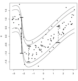
where atan2[y,x] is the angle between the x-axis and the vector from the origin to (x,y). We will estimate quantiles of orders 0.01,0.05,0.95,0.99 in correspondence of these three values of the conditioning variable: −2.2,−1.5,1.5. These latter values are chosen to consider a variety of slopes. A single example is given in Figure 1 for sample size n =100, which shows the estimates at the given design points together with the theoretical quantiles, which are of constant width.
We note that the estimator (5) depends on a pair of smoothing parameters (say (κ, λ1)), whereas (10) depends only on one (sayλ2) which would suggest that the double-kernel estimator will provide more flexibility, at the expense of potential difficulty in using cross-validation to select appropriate values.
As a second simulation experiment, for each n ∈ {50,100,500}we simulated 100 samples. In each case we obtained quantile estimates, corresponding to the same orders and conditioning variable values as the first experiment,
using (5) for a grid of values of (κ, λ1) and (10) for a grid of values ofλ2. The results from the simulations were combined by using a sample version of the accuracy measure (6).
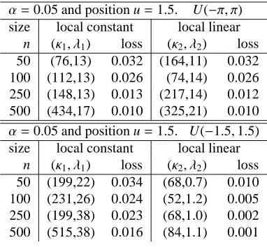
Three sets of results are shown. In the first set we fix n=100 and u=1.5 and considerα∈ {0.01,0.05,0.95,0.99}, In the second set, we take n=100 andα=.05 and consider u∈ {−2.2,−1.5,1.5}. In the third set, we takeα=0.05 and u = 1.5 and consider n ∈ {50,100,250,500}. In each set we report: the values of (κ, λ1) which maximize the accuracy for estimator (5), together with the corresponding loss, and the value ofλ2 which maximizes the accuracy for (10), with its corresponding loss. The results are presented in Table 1.
−3 −2 −1 0 1 2 3
−1.5
−1.0
−0.5
0.0
0.5
1.0
1.5
quantile estimation for simulated data: example
u
θ
−
−
−
−
−
[image:10.612.157.426.183.465.2]−
Figure 1: Theoretical quantiles (lines) forα∈ {0.01,0.05,0.95,0.99}for the von Mises model with conditional mean given by (13) andκ=10.
n=100 points are generated from this model, in which u is uniform on the circle. As an illustration, the check quantile estimates (10) are shown forα{0.01,0.99}(continuous) andα{0.05,0.95}(dashed) at locations u∈ {−2.2,−1.5,1.5}. In this illustration we have chosenλ=100.
Firstly we note that, as expected, estimator (5) is a little better than (10) in all settings. However, the improvement comes at a computational price. The first set of results shows a similar performance for each of the quantile estimates. In the second set, we can see that estimating quantiles at u=−2.2 is more difficult than either of the other locations. At this position there is a steep gradient over a small interval, and so little information is available. Correspondingly, much larger values ofλ1andλ2are selected at this position. Finally, the dependence on sample size is also much as expected; there is improving accuracy with n and a general increase in concentration parameters.
5.2. Local constant and local linear estimators
We use similar settings as in the third block of Table 1 in that we consider u=1.5 andα=0.05 for various values of n, and continuing to use the same conditional mean function (eq:simmean). Here, we also consider the same local constant estimator (5) but now we compare this to the corresponding local linear estimator, based on (2), in the case that the explanatory variable is uniform on the circle (as before), and in the case when it is uniform on (−1.5,1.5) so that we are estimating the quantile at the boundary of the sample space. The results are shown in Table 2.
position u=1.5 and sample size n=100 quantile estimator (5) estimator (10)
α (κ, λ1) loss λ2 loss
0.01 (33,31) 0.028 16 0.049
0.05 (48,20) 0.025 10 0.032
0.95 (116,11) 0.022 10 0.026
0.99 (11,18) 0.022 7 0.027
quantileα=0.05 and sample size n=100 position estimator (5) estimator (10)
u (κ, λ1) loss λ2 loss
−2.2 (43,300) 0.082 194 0.094
−1.5 (29,17) 0.025 6 0.037
1.5 (57,17) 0.030 11 0.037
quantileα=0.05 and position u=1.5 size estimator (5) estimator (10)
n (κ, λ1) loss λ2 loss
50 (34,13) 0.030 9 0.039
100 (175,10) 0.026 9 0.030
250 (210,13) 0.011 12 0.011
[image:11.612.200.394.98.348.2]500 (246,19) 0.009 13 0.011
Table 1: Results of three simulation sets from model (13), for various settings of sample size n, location u and quantilesα(see Figure 1 for an example). In each setting, we report the optimal pair (κ, λ1) orλ2for estimators (5) & (10), respectively with corresponding minimized loss (6).
Results were obtained from 100 samples in each setting.
α=0.05 and position u=1.5. U(−π, π)
size local constant local linear
n (κ1, λ1) loss (κ2, λ2) loss
50 (76,13) 0.032 (164,11) 0.032
100 (112,13) 0.026 (74,14) 0.026
250 (148,13) 0.013 (217,14) 0.012
500 (434,17) 0.010 (325,21) 0.010
α=0.05 and position u=1.5. U(−1.5,1.5)
size local constant local linear
n (κ1, λ1) loss (κ2, λ2) loss
50 (199,22) 0.034 (68,0.7) 0.010
100 (231,26) 0.024 (52,1.2) 0.005
250 (199,38) 0.023 (68,1.0) 0.002
500 (515,38) 0.016 (84,1.1) 0.001
Table 2: Results of two simulation sets from model (13), for various settings of sample size n. In each row, we report the optimal pair (κ, λ) for the estimator (5) based on (1) and (2), respectively with corresponding minimized loss (6). Results were obtained from 100 samples in each setting. In the top block the explanatory variable is uniform on the circle (and a repeat of the last block of Table 1) and in the second block, U is uniform on (−1.5,1.5).
[image:11.612.202.393.414.591.2]We can see that the performance is quite similar between the local constant and the local linear in the case that the quantile is estimated at an interior point. However, in the case that the explanatory variable has limited support and the quantile is estimated at a boundary, then the local linear estimator performs much better, and the improvement increases with sample size. This is as expected.
We note that in all double-kernel experiments, the choice ofλwas much more important than the choice ofκ.
6. Application
We illustrate the estimation of a conditional circular distribution function using some data on wind speed and wind directions. The data, which is taken from an observation station close to the Florida coastline and was collected by the National Data Buoy Center of the NOAC, is intended to illustrate the potential uses of the methodology.
The first part of our analysis concerns finding an “optimal” direction corresponding to wind speeds near to a specified value. Then we consider conditional quantile estimation, and assess its coverage. Note that any concern about where to “cut” the circle is not an issue in the questions we address here.
6.1. Estimation of optimal direction
A wind rose is often used to display information about the direction of particular wind speeds, and Figure 2 shows some sample rose diagrams revealing the distribution of wind directions corresponding to wind speeds 9 m/s and 12 m/s. We initially note that our method is not hampered by an arbitrary, equi-spaced partition of the circle as rose diagrams are.
wind directions for speed 9
90
270
180 0
wind directions for speed 12
90
270
[image:12.612.104.502.325.529.2]180 0
Figure 2: Rose diagrams for wind directions corresponding to the observed wind speeds (m/s) in the range (8,10) (left) and (11,13) (right).
This type of data is highly relevant to the analysis of proposed wind turbine installations. The energy (and revenue) generated by a wind turbine is crucially dependent on the wind speed; different turbines may have different (energy– wind speed) response rates. Locations with little wind will often be uneconomic, and locations with very high wind speeds will cause different problems. By considering the wind speed and wind direction distributions, the anticipated energy may be calculated. Our dataset consists of wind speed and wind directions at a specific location so in this illustration U, which represents the wind speed, is linear, andθ∈[−π, π) is the direction.
We will suppose that the energy output for a proposed turbine is highest for wind speeds close to some w m/s and we are interested to know the direction of the turbine which will “optimize” the energy. If we suppose that the turbine
will function within an angle ofπ/4 radians of the wind, then we need to find a directionθ=θ(w) to maximize
F(θ(w)+π/4|u=w)−F(θ(w)−π/4|u=w).
We can estimate this using Equation (1), in which the weights L can be based on either a local constant, or local linear estimate. One way to select the smoothing parameters (λandκ) is to consider the mean squared error of the estimates, and then use the results of Theorems 3 and 4. This would require suitable plug-in methods, similar to those of Yu and Jones (1998), who deal with analogous linear methods. Bandwidth selection for simple directional density estimation as, for example, in Garc´ıa-Portugu´es (2013), would be inappropriate in this setting. However, in our application the choice ofλis practically determined by consideration of the fact that we actually want to estimate F(θ(w)+π/4|u≈w)−F(θ(w)−π/4 |u ≈w) and so (this will often depend on the operating characteristics of the specific turbine) we have consideredλ=0.6 andλ=1.2 in our calculations with a normal kernel for Kλ(soλis the
standard deviation). Given the choice of normal kernel, these choices ofλwere chosen to focus on a range of wind speeds of about±2λ. Our illustrative data consists of 17,480 observations, with wind speeds which range from 0.1 m/s to 18 m/s (mean 5.9).
4 6 8 10 12 14
2.5
3.0
3.5
4.0
4.5
5.0
5.5
optimal turbine direction (NW estimate)
wind speed (w)
optimal direction (mod 2
π
)
λ
naive κ
10 100
0.6
1.2
4 6 8 10 12 14
2.5
3.0
3.5
4.0
4.5
5.0
5.5
optimal turbine direction (LL estimate)
wind speed (w)
optimal direction (mod 2
π
)
λ
naive κ
10 100
0.6
1.2
Figure 3: Wind turbine direction to maximize output using an estimate of the conditional CDF based on Equation (1). Four smoothed estimates (dependent onλandκ) are shown, as well as a naive estimate, for each of local constant (left) and local linear (right) estimation.
Some results are presented in Figure 3, where the dependence of the optimal direction on the wind speed can be clearly seen. The dependence onκis small, as is the effect ofλon the result. For ease of interpretation, we have used angles mod(2π) to avoid “wrapping”. We have also considered a naive approach for comparison. In this case, we chose the angle (θ0=θ0(w)) to maximize
X
{i:wi∈(w−1,w+1)}
1{cos(θ0−θi)>1/√2},
and the result is shown on both plots. This naive estimate is more akin to a histogram, though the resulting values of
θ0are still quite smooth, with all estimates showing a similar overall structure. Figure 3 shows a marked difference in the optimal direction between wind speeds 9 m/s (where the optimal direction is about 3.5 radians) and 12 m/s (with optimal direction about 5.3 radians).
6.2. Conditional quantile estimation
Estimation of specific quantiles will depend on the choice of ”cut point” on the circle, so we avoid this arbitrary selection by considering the estimation of confidence intervals conditional on wind speed, and investigate the potential
to chooseλandκby cross-validation. Ideally, this should be considered with respect to a loss function which measures the coverage accuracy for a specific set of quantiles. However, since the coverage is discrete, this typically results in a cross-validation function which is piecewise constant, and harder to optimize. Instead, we again consider estimation of the conditional CDF as a means to get suitable smoothing parameters, and we use an adaptation of Equation (2) in Di Marzio et al. (2012), so thatλandκare chosen to minimise
CV(κ, λ|u)= X
i:Ui≈u
Z π
−π
n
1{θ≥θi}−Fˆλ,κ(i)(θ|u)
o2
dθ (14)
where ˆFλ,κ(i)(·) is the smoothed estimate (1) of the conditional CDF using all the data except the ith observation, with smoothing parametersκ andλ. There are two points to note here. Firstly, the smoothing parameter selection does not take any account of the quantile(s) to be estimated, although the parameters do depend on the wind speed (u). Secondly, there is a need to make precise what “≈” means in the limit of the summation in Equation (14). In our example, the wind speeds are recorded to one decimal place, but in general one will require a sufficient number of observations in order to achieve stable results.
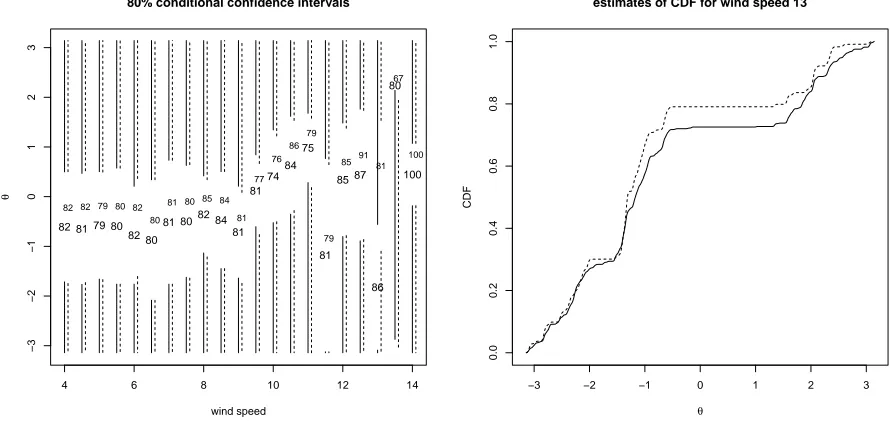
For given wind speeds, we first find the smoothing parameters by using Equation (14) for both local linear and local constant estimators. Then, using these smoothing parameters we compute (1). Finally, for givenαwe choose an “origin” to minimise the width of the interval, which leads to estimates of the “lower” and “upper” endpoints. This final step is used to avoid the somewhat arbitrary choice of origin, or ”cut point” for data which lie on a circle. In Figure 4 we show the 80% confidence intervals corresponding to the distribution of the direction conditional on wind speed. Also on this plot, we give the actual coverage, as a percentage, for both the local constant, and local linear estimates. Although the coverages are mostly close to 80% (as desired) it should be remembered that the data is not independent of the cross-validation data. The intervals (and coverage) are quite similar for the two methods, except for wind speed 13 m/s; the estimates of the conditional CDFs for this wind speed are also shown.
4 6 8 10 12 14
−3
−2
−1
0
1
2
3
80% conditional confidence intervals
wind speed
θ
82 81 79 80 82 80
81 808284
81 81
74 84
75
81 85 87
86 80
100
82 82 79 80 82 80
81 80 85 84 81
77 76
86 79
79 859181
67
100
−3 −2 −1 0 1 2 3
0.0
0.2
0.4
0.6
0.8
1.0
estimates of CDF for wind speed 13
θ
[image:14.612.66.511.373.586.2]CDF
Figure 4: Left: 80% confidence interval estimates of direction conditional on wind speed for local linear (lines) and local constant (dashed). The numbers give actual coverage for each method; the larger font is used for local linear, and the smaller for local constant. Note that the intervals are shown by vertical lines (not by the gaps). Right: the estimated conditional CDF for wind speed 13 m/s for local linear (lines) and local constant
(dashed).
7. Discussion
We should stress that in any practical application the choice of origin (“cut-point”) should be chosen dependent on u to minimise the width of the interval to be estimated. This adjustment is important to obtain meaningful inter-pretations, especially if the conditional mean can take values close toπ. We note that the double-kernel estimator has two tuning parameters (λandκ) whereas the circular check function estimator has only one. Maybe, it is for this rea-son that, in some simulation experiments with small samples, we have observed a slightly better performance for the double-kernel estimator in most settings. However, this comes with the cost of more computational effort, as well as the need to select good smoothing choices. This effort can be reduced by first selecting a good value ofλin the check function, and then using this value, together with an appropriateκ, in the double-kernel estimator. Cross-validation can be used in this process, though we have found a joint selection of bothκandλto be problematic.
References
Berg, A. and Politis, D. CDF and survival function estimation with infinite-order kernels. Electronic Journal of Statistics, 3, 1436–1454 (2009). Di Marzio, M., Panzera, A. and Taylor, C. C. Local polynomial regression for circular predictors. Statistics&Probability Letters, 79, 2066–2075
(2009)
Di Marzio, M., Panzera, A. and Taylor, C. C. Density estimation on the torus. Journal of Statistical Planning and Inference, 141, 2156–2173 (2011) Di Marzio, M., Panzera, A. and Taylor, C. C. Smooth estimation of circular distribution functions and quantiles. Journal of Nonparametric Statistics,
24, 935–949 (2012)
Fan, J., Hu, T. and Truong, Y. K. Robust Non-parametric Function Estimation. Scandinavian Journal of Statistics, 21, 433–446 (1994)
Garc´ıa-Portugu´es, E. Exact risk improvement of bandwidth selectors for kernel density estimation with directional data. Electronic Journal of
Statistics, 7, 1655–1685 (2013)
Jones, M.C. and Hall, P. Mean squared error properties of kernel estimates of regression quantiles. Statistics&Probability Letters, 10, 283–289
(1990)
Jones, M.C. and Noufaily, A. Parametric quantile regression based on the generalised gamma distribution. Journal of the Royal Statistical Society,
Series C, 62, 723–740 (2013)
Li, Q. and Racine, J. S. Nonparametric estimation of conditional CDF and quantile functions with mixed categorical and continuous data. Journal
of Business&Economic Statistics, 26, 423–434 (2008)
Yu, K. and Jones, M.C. Local linear quantile regression. Journal of the American Statistical Association, 441, 228–237 (1998)
Appendix
Proof of Theorem 1 Observing that estimators (1) and (2) can be respectively regarded as a local constant and local
linear estimators of
m(θ, φ)=E[Wκ(θ−Θ)−Wκ(−π−Θ)|Φ =φ],
in virtue of assumptions i) and iii), Theorem 4 of Di Marzio et al. (2009) gives
E[ ˆFλ,κ(θ|φ)]−m(θ, φ)=
η2(Qλ)
2
n
m(0,2)(θ, φ)+2gg(′(φφ))m(0,1)(θ, φ)o+o(η2(Qλ)), f or estimator (1);
η2(Qλ)
2 m
(0,2)(θ, φ)+o(η
2(Qλ)), f or estimator (2);
and, for both estimators,
Var[ ˆFλ,κ(θ|φ)]=
R(Qλ)s2(φ, θ)
ng(φ) +o(η2(Qλ)),
where s2(θ, φ)=Var[W
κ(θ−Θ)−Wκ(−π−Θ)|Φ =φ].
Now, notice that m(θ, φ) and s2(θ, φ) respectively amount to expectation and variance of the circular CDF estimator provided by Di Marzio et al. (2012), conditional onΦ = φ. Thus, an adaptation of the results stated in Theorem 2.1 of Di Marzio et al. (2012), for the unconditional case, along with assumption ii), yield
m(θ, φ)=F(θ|φ)+ 1 2k{F
(2,0)(θ
|φ)−F(2,0)(−π|φ)}+o(κ−1), (15)
and
s2(θ, φ)=F(θ|φ){1−F(θ|φ)} − √1
πk{F (1,0)
(θ|φ)−F(1,0)(−π|φ)}+o(κ−1/2). (16)
Hence, by plugging (15) and (16) in the expectations and variance expressions, the results follow.
Proof of Theorem 2 The results follow by using the same arguments as in the proof of Theorem 1, once observed
that, in virtue of assumption i), euclidean local polynomial fitting theory gives
E[ ˆFλ,κ(θ|x)]−m(θ,x)=
λ2µ
2(Q)
2
n
m(0,2)(θ,x)+2g′(x)
g(x)m
(0,1)(θ,x)o
+o(λ2), f or estimator (1);
λ2µ
2(Q)
2 m
(0,2)(θ,x)+o(λ2), f or estimator (2);
and, for both estimators,
Var[ ˆFλ,κ(θ|x)]=
R(Q)s2(x, θ)
nλg(x) +o
1 nλ
!
.
Proof of Theorem 3 First observe that, by standard Taylor series arguments, we can write
E[2{1−cos( ˆqα,λ,κ(u)−qα(u))}]≈E[{ˆqα,λ,κ(u)−qα(u)}2]
={E[ ˆqα,λ,κ(u)−qα(u)]}2+E[{ˆqα,λ,κ(u)−E[ ˆqα,λ,κ(u)}2]
Now, using the approximation
ˆqα,λ,κ(u)−qα(u)≃ −
ˆ
Fλ,κ(qα(u)|u)−F(qα(u)|u) f (qα(u)|u)
,
Theorem 1 when u=φand Theorem 2 when u=x, along with F(qα(u)|u)=α, yield the result.
Proof of Theorem 4 The result directly follows by using the same arguments as in the proof of Theorem 3, along
with results of Theorem 1 when u=φ, and Theorem 2 when u=x.
Proof of Theorem 5 Reasoning as in Jones and Hall (1990), define
Hα(u)=
1 n
n
X
i=1
Qλ(Ui−u){α1{β<Θi<π}−(1−α)1{−π<Θi<β}},
obtaining that
E[Hα(u)|U1,· · · ,Un]=
1 n
n
X
i=1
Qλ(u−Ui){α−F(β|Ui)}.
Now, expanding F(β|Ui) in Taylor series, for (β,Ui) around (qα(u),u), it results
F(β|Ui)≈F(qα(u)|u)+{β−qα(u)}f (qα(u)|u)+ Ψ(Ui−u)F(0,1)(qα(u)|u)+
1 2Ψ
2
(Ui−u)F(0,2)(qα(u)|u),
and using similar approximations as those used in the proof of Theorem 3, we finally get
E[Hα(u)]=−{β−qα(u)}f (qα(u)|u)g(u)− ξ(Qλ)
2
2F(0,1)(q
α(u)|u)g′(u)+F(0,2)(qα(u)|u)g(u) +o(ξ(Qλ))
Moreover, reasoning again as in Jones and Hall (1990), we have
Var[Hα(u)]=
ν(Qλ)g(u)
n α(1−α)+o
ν(Qλ) n
!
.
Now, use the fact that{Var[Hα(u)]}−1/2{Hα(u)−E[Hα(u)]}converges to a standard normal distribution, and that
estimator (9) is the solution forβof Hα(θ)−E[Hα(u)]=−E[Hα(u)].
Proof of Theorem 6 When u∈[0,1], the result directly follows by using Theorem 3 in Fan et al. (1994), withλin
place of h. When u is an angle, the same result holds, with due modifications, by using the assumptions in Theorem
5.