Ultra-Orthogonal Forward Regression Algorithms for the Identification of Non-Linear Dynamic Systems

This is a repository copy of

Ultra-Orthogonal Forward Regression Algorithms for the

Identification of Non-Linear Dynamic Systems

.

White Rose Research Online URL for this paper:

http://eprints.whiterose.ac.uk/107310/

Version: Accepted Version

Article:

Guo, Y, Guo, LZ, Billings, SA et al. (1 more author) (2016) Ultra-Orthogonal Forward

Regression Algorithms for the Identification of Non-Linear Dynamic Systems.

Neurocomputing, 173 (3). pp. 715-723. ISSN 0925-2312

https://doi.org/10.1016/j.neucom.2015.08.022

[email protected] https://eprints.whiterose.ac.uk/ Reuse

This article is distributed under the terms of the Creative Commons Attribution-NonCommercial-NoDerivs (CC BY-NC-ND) licence. This licence only allows you to download this work and share it with others as long as you credit the authors, but you can’t change the article in any way or use it commercially. More

information and the full terms of the licence here: https://creativecommons.org/licenses/

Takedown

If you consider content in White Rose Research Online to be in breach of UK law, please notify us by

1

Ultra Orthogonal Forward Regression Algorithms for the

Identification of Non-Linear Dynamic Systems

Revised 20.07.2015

Yuzhu Guo, L.Z. Guo, S. A. Billings, and Hua-Liang Wei

Department of Automatic Control and Systems Engineering

The University of Sheffield, Mappin Street, Sheffield, S1 3JD, UK.

INSIGNEO institute for in silico Medicine

The University of Sheffield, Mappin Street, Sheffield, S1 3JD, UK.

Abstract

A new Ultra Least Squares (ULS) criterion is introduced for system identification. Unlike the standard least squares criterion which is based on the Euclidean norm of the residuals, the new ULS criterion is derived from the Sobolev space norm. The new criterion measures not only the discrepancy between the observed signals and the model prediction but also the discrepancy between the associated weak derivatives of the observed and the model signals. The new ULS criterion possesses a clear physical interpretation and is easy to implement. Based on this, a new Ultra Orthogonal Forward Regression (UOFR) algorithm is introduced for nonlinear system identification, which includes converting a least squares regression problem into the associated ultra least squares problem and solving the ultra least squares problem using the orthogonal forward regression method. Numerical simulations show that the new UOFR algorithm can significantly improve the performance of the classic OFR algorithm.

Key words: orthogonal forward regression, system identification, ultra least squares, ultra orthogonal forward regression, ultra orthogonal least squares.

1. Introduction

2 used to evaluate the performance of each model by measuring the discrepancy between the observed data and the model predictions. The candidate model dictionary is often chosen to be large enough to include the unknown correct model. Hence an exhaustive search algorithm is often infeasible in these kinds of applications because of the large solution space. Even an evolutionary algorithm which can greatly reduce the search process can still be very computationally intensive. Hence an algorithm which can efficiently find the optimal solution is desired. However, a fast algorithm often dictates an optimal substructure; otherwise the search may converge to a suboptimal solution. Many efforts have been made to improve the search process under a certain specific loss function or performance index, for example, the simulated annealing algorithm, particle swarm optimisation, and so on. In this paper, a different and new methodology will be introduced. Instead of improving the search method, a new and effective criterion will be introduced to describe the objective of the regression more accurately. Under the new criterion, the solution space has a better structure and a fast algorithm is more likely to find the optimal solution.

System identification aims to identify a model from observed data based on a criterion. A good criterion results in not only better parameter estimation but also a good search path along which the search process converges quickly to the optimal solution. Over the years, different criteria have been used in system identification such as the 2

L norm in least squares regression, the 1

L norm in least absolute value regression (Bloomfield & Steiger, 1980; Narula & Wellington, 1982), and zero-norm minimisation (Kaizhu, King, & Lyu, 2008), etc. Among these criteria, the least squares criterion is the most used because of its excellent properties, for example, least squares estimation can be configured to give estimates which are unbiased and efficient when the noise satisfies some basic assumptions. Least squares problems have analytic solutions and can easily be solved using the QR decomposition technique, and least squares regression produces unique and numerically robust solutions. Consequently a large number of system identification algorithms based on the least squares criterion have been developed (Billings, 2013; Li, Peng, & Bai, 2006; Ljung, 1987; Söderström, 1989).

3 to over-fitted models in least squares regression, which can be seen in the motivational example described in Figure 1 and discussed in the next section.

The standard least squares regression investigates the problem of model fitting on the space

[ ]

(

)

2

0,

L T , where

[ ]

0,T represents the time span of a signal. The associated Residual Sum of Squares (RSS), which is the square of the 2

L norm of the residual, is used to measure the fitness of the model.

When the model structure is known, the standard least squares algorithm produces the best

parameters with which the model will be optimal in the sense of RRS. Considering different model

structures, there are plenty of very different models which give the same fitness for a set of

observed data in the sense of the RSS criterion. In this paper, an alternative criterion, called ultra least squares (ULS) criterion will be introduced to characterise the model fitness more accurately. Unlike the least squares criterion consider the model fitting on the space 2

L , the ULS criterion considers the model fitting in a smaller space, more specifically, the Sobolev space m

(

[0, ]

)

H T (Maz'ia, 1985). The norm defined on this space will be modified and used as the ULS criterion for system identification, where not only residuals but also the associated weak derivatives will be used to measure the model fitness.

Using the derivatives of the data in system identification has been studied, especially in the identification of continuous time models (Brewer, Barenco, Callard, Hubank, & Stark, 2008; Preisig & Rippin, 1993; Schmidt & Lipson, 2009). However, as far as the authors are aware this study is the first time the weak derivatives have been combined with the least squares criterion to build a completely new metric for the prediction errors and which uses the new metric to improve the model structure detection in non-linear system identification.

In this paper, the ULS criterion will be combined with the well known Orthogonal Forward Regression (OFR) algorithm (Billings, 2013) to construct a new Ultra Orthogonal Forward Regression (UOFR) algorithm for nonlinear system identification. The proposed UOFR algorithm is shown to be very powerful for model structure detection in many modelling tasks and is more likely to produce an optimal model.

The remainder of the paper is organised as follows: Section 2 briefly reviews some main results on the Lebesgue space 2

L and the Sobolev space m

H . The ULS criterion will be presented by modifying the m

4

2. Problems of least squares regression and model fitting in Sobolev

space

In this section, a motivational example is first given to show the problems that can arise when using a standard least square criterion. The reasons which cause these problems will then be discussed in detail and an alternative criterion will be proposed.

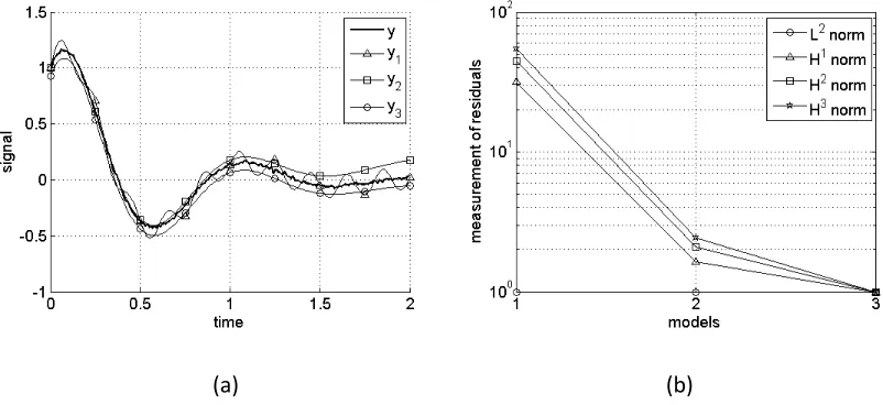
Consider the time series fitting problem shown in Figure 1. In this example, three models were identified from an observed signal ywhich is represented by a thick solid line in Figure 1(a). The reproduced signals by the three models are represented by the curves y₁, y₂, and y₃ in the Figure 1(a) respectively. Figure 1(b) shows the different measurements of the model fitness of the three models: the 2

L norm and the m

H

(

m=1, 2,3

)

norms of the residuals.

From Figure 1(b), it can be observed that the three models give the same fitness in the sense of the least squares criterion, which is presented by the line with the circle marks along the abscissa in 1(b), although the reproduced signal y₁ looks significantly different from y₂ andy₃ in 1(a).

[image:5.595.92.493.389.573.2]

(a) (b)

Figure 1 A motivational example for model fitting of a noisy signal

(a) Observed data and reproduced signals for three different models (b) measurement of the fitness of the

models using different criteria

Figure 1 (b) shows also the measurements of the errors in the sense of m

H norms when m=1, 2, 3. It can be observed that the performances of the three models under the m

H norms are significantly different. Model 3 fitted the signal y better than models 1 and 2 did. The system identification problems consists of finding the function on m

(

[0, ]

)

5

2, …, N, where both the data points and the interconnections among the datum points (described by the weak derivatives) are considered.

This example shows that the least squares criterion which defined on the 2

L space neglects some very important information in the observations. This information is crucial for identifying a correct model. Alternatively, the model fitness can more accurately be characterised on a smaller space, the Sobolev space m

H , which consists of all the functions which are 2

L integrable and the where up to

mth weak derivatives exist and are also 2

L integrable. The new introduced ULS criterion is a realisation of the m

H norm based on the observations.

The generic least squares regression problem includes determining the structure of a linear-in-the-parameters model and estimating the associated coefficients

1

i i i

y x e

κ

θ

=

=

∑

+ (1)

via minimising the loss function

2

1 2

LS i i

i

J y x

κ

θ

=

= −

∑

. (2)

The aim is to produce a parsimonious model, where y represents the dependant variable and the

i

x ’s are the explanatory variables. In the system identification of dynamic systems, the y and x_i’s are time dependent signals with finite energy, that is, these signals are 2

L integrable functions in the Lebesgue space 2

(

[ ]

)

0,

L T , where

[ ]

0,T is the time span of the signals. Least squares regression involves finding a model to minimise the square of the 2

L norm (2). Although the least squares loss function is defined based on the 2

L norm, the signals in a dynamic system are more regular than a general 2

L function because of the fact that most physical systems behave essentially as a low-pass filter. These signals are actually functions defined on the subspace of 2

(

[ ]

)

0,

L T , specifically, the Sobolev space

(

)

,2

(

)

[0, ] [0, ]

m m

H T =W T (Maz'ia, 1985)

(

)

{

( )

2

(

[ ]

)

2

(

[ ]

)

}

[0, ] 0, 0, , 1, 2, , ,

m l

H T = x t ∈L T D x∈L T l= ⋯ m ₍₃₎

which is the space of functions defined on [0, ]T , the weak derivatives up to mth order are also 2

L

integrable and t represents continuous time. The weak derivatives l

( )

D x t satisfy

( )

( )

( )

[0, ] ( ) ( ) 1 [0, ]

l

l l

T x t Dϕ t dt= − Tϕ t D x t dt

6 for any test functionϕ

( )

t ∈C₀∞

(

[ ]

0,T

)

, which is smooth and possesses compact support on [0, ]T .

The metric in 2

(

[ ]

)

0,

L T space is defined by the Lebesgure integral. Hence the distance

2

ˆ

x−x , which measures the differences on the interval

[ ]

0,T between functions x t

( )

and ˆx t

( )

as a whole, cannot characterise how the differences are distributed at each time instance. As a result, the 2

L norm only emphasises the similarity of two functions as a whole but disregards the closeness or detail in shape. System identification can be interpreted as discovering unknown rules from a set of observations. Every piece of information can be crucial for a method to discover the correct rules, especially when the system is not persistently excited, where many important system characteristics are not fully excited and are inconspicuously contained in a small number of data. The absence of this information can lead to a wrong model structure. However, this unapparent information can easily be overshadowed by a large amount of trivial data in a global criterion such as the 2

L norm. Therefore, an unclear objective function may confuse system identification algorithms and increase the algorithms sensitivity to noise. Nuances in the data may therefore cause the algorithms to produce incorrect models. Hence a stricter criterion which can accurately characterise the objectives of system identification and reveal all the useful information in data should be investigated.

A stricter metric for the Sobolev space m

(

[0, ]

)

H T is the norm defined as

2 2 0

m m

l H

l

x D x

=

=

∑

, (5)

where l

D represents the lth differentiation operator.

Based on the above norm, a new criterion can then be defined as

2 2

1 2 1 1 2

m l

H i i i i

i l i

J y x D y x

κ κ

θ θ

= = =

 

= − +  − 

 

∑

∑

∑

. (6)

Due to the fact that the differentiations are linear operators, the above criterion can be written as

2 2

1 2 1 1 2

m

l l

H i i i i

i l i

J y x D y D x

κ κ

θ θ

= = =

= −

∑

+

∑

−

∑

. (7)

7 which can reveal more information by introducing the second term, is an alternative criterion to the pure least squares criterion. In the next section, an ULS criterion will be derived by adapting the J_H

criterion to the nonlinear system identification problem. Next, two theorems about the relationships between the 2

L and m

H spaces and the associated norms will be given to show that the Sobolev space m

H is an appropriate space, and the associated norm is an appropriate criterion for a least squares problem.

Theorem 1. For any approximation 2

(

[ ]

)

ˆ 0,

y∈L T to a function y in 2

(

[ ]

)

0,

L T satisfying y−yˆ ₂≤ε, there exists an yɶ∈Hm

(

[ ]

0,T

)

satisfying

2

y−yɶ ≤γεfor any γ >1. This theorem can easily be proved from the result that m

H is dense in 2

L so that there exists a function yɶ in m

H subject to yɶ−yˆ ₂ <

(

γ−1

)

ε . Based on Minkowski’s inequality y−yɶ ₂ =

2

ˆ ˆ

y− + −y y yɶ ≤ −y yˆ ₂+ −yˆ yɶ ₂.

Theorem 1 shows that there exists an approximation in m

H which is not significantly different from an approximation ˆy in 2

L but is more regular. Therefore, the Sobolev space _Hm

(

[ ]

0,_T

)

_{is smaller}

than the 2

(

[ ]

)

0,

L T space but large enough for a least squares approximation. Theorem 2. For any small positive real number ε, m

H

y−yɶ <ε means

2

y−yɶ <ε. Proof:

The result is straightforward because

2

2 2

2 2 2 2

1

. m

m

l l

H

l

y y y y D y D y y y x

=

− ɶ = −ɶ +

∑

− ɶ ≥ − ɶ = ₍₈₎

Hence, for any small positive number ε>0, y−yɶ ₂ ≤ −y yɶ _Hm <ε. This proves the theorem. □

Theorem 2 indicates that the J_H criterion is a stricter than the least squares criterion. If a model fits the data well in the sense of J_H, the model is also good in the sense of least squares. The reverse is not true.

8 Definition 1. Under the new m

H norm, the least squares problem (1) is equivalent to a new least squares problem 1 1 1 i i i i m m i x y D x D y D x D y κ θ =            ₌            

∑

_⋮

⋮ . (9)

The new least squares problem (9) will be defined as the ultra least squares problem corresponding to the original least squares problem. The solution of the ultra least squares problem will be referred to as the ultra least squares solution of the original least squares problem.

The ultra least squares solution can be obtained by solving the ultra least squares problem. However, some more work is still needed before this can be used for data-driven system identification problems. Firstly, the weak derivatives are usually not known in many system identification problems. Secondly, the contribution of each component

2

1 2

l l

i i i

D y D x

κ

θ

=

−

∑

to the J_H criterion may

not be balanced. The differentiation terms

2

1 2

l l

i i i

D y D x

κ

θ

=

−

∑

may magnify the effects of noise and incorrectly dominate the J_H criterion. Consequently, J_H criterion will not be robust to noise. Thirdly, the m

H norm looks quite mathematical when it would be preferable that the identification process is physically easy to understand and computationally cheap.

In order to evaluate the contribution of the unknown weak derivatives in the J_H criterion, the distributions corresponding to the signals y and x_i will be introduced. For the signal y t

( )

, the associated distribution T_y can be defined as a functional Ty:C₀

(

[0, ]T

)

R

∞ _→

( ) ( )

[0, ]

,

y _T

T ϕ =

∫

y t ϕ t dt (10)

for all ϕ∈C₀∞

(

[0, ]T

)

. The distribution T_y now has weak derivatives which are defined as

( )

( )

( )

_{( )}

[0, ]

, 1l l

l

y _T

D T ϕ = −

∫

y t ϕ t dt. (11)

Similarly, the distributions corresponding to x_i can be defined as

( ) ( )

[0, ]

, i

x _T i

9 The regression is now solved in the sense of distribution. The system identification problem involves fitting the distribution T_y by the combination of a set of distributions

i x

T ’s. The ultra least squares problem (9) then becomes

1 1 , , , , i l y x i i m l y x y x

D T D T

D T D T

κ ϕ ϕ θ ϕ ϕ =             =                

∑

⋮ ⋮ , ϕ C0

(

[ ]

0,T

)

∞

∈ (13)

Data can be collected by evaluating the values of these distributions for different test functions ϕ

( )

t in C₀∞

(

[0, ]T

)

. The regression matrix can then be constructed and the parameters can be estimated based on the regression matrix.

However, there are not a finite number of functions which form a basis of C₀∞

(

[0, ]T

)

. Hence, it is infeasible to evaluate the values of the distributions over the whole C₀∞

(

[0, ]T

)

space. A trade-off is needed between incorporating all the information of the distributions in the ULS problem and computational efficiency.

The weak derivatives of a function based on a locally defined test function ϕ

( )

t reveal the local information of the function. Shifting the test function along the time axis yields different test functions and the associated weak derivatives contain local information of the signal at the new positions. Instead of all the test functions in C₀∞

(

[0, ]T

)

, a locally defined test function ϕ

( )

t and time shifts ϕ

(

t−τ

)

are used in the following discussion.

Given a test function ϕ

( )

t with a finite support on

[ ]

0,T0 , T0<T , the ultra least squares problem

can then be approximately described as

(

)

(

)

(

)

(

)

1 1 1 , , , , i i i x y i i m m y x x y

D T t

D T t

D T t D T t

κ ϕ τ

ϕ τ

θ

ϕ τ ϕ τ

=         − −     =            ₋  ₋    

∑

⋮ ⋮ , τ∈

[

0,T−T0

]

(14)

(

) ( )

( )

( )

₍

₎

[ ]0,

, 1l l

l y

T

D T ϕ t−τ = −

∫

y t ϕ t−τ dt (15)

The distribution m ,

(

)

y

10

( )

(

) ( )

( )

( )

₍

₎

0

, 1l T l

l l

y

y τ ≜ D T ϕ t−τ = −

∫

y t ϕ t−τ dt. (16) Here l

( )

y τ is the convolution of the signal y t

( )

with the lth derivative of a function which is defined as g t

( )

≜ϕ

( )

−t . The weight function ( )l

( )

g t can then be thought as the impulse response of a linear filter and l

( )

y τ is the output of the filter to the input y t

( )

.

According to Leibniz integral rule, differentiation under the integral sign satisfies

( ) (

)

( )

(

)

( )

(

)

0 0 0

l l l

t t t

l l l

d d

y g t d y g t d y g t d

dt τ τ τ τ t τ τ τ dt τ τ

∂

− = − = −

∂

∫

∫

∫

(17)

That is, the order of the differentiation and the integral can be interchanged. Now the newly introduced functions l

( )

y τ have a new physical interpretation. The function l

( )

y τ

represents a signal which is obtained from the original signal y t

( )

through two steps: the signal

( )

y t is initially smoothed by a filter with an impulse response g t

( )

, the smoothed signal then passes through an lth order pure differentiation system. This is equal to smoothing the signal first and then calculating the derivatives of the smoothed signals.

Similarly, the functions l

( )

i

x τ can be defined as

( )

(

) ( )

( )

( )

₍

₎

0

, 1

i

T

l l

l l

i x i

x τ ≜ D T ϕ t−τ = −

∫

x t ϕ t−τ dt (18)

The ULS problem (14) then becomes

1 1

1

i

i i i

m m

i x y

x y

x y

κ

θ

=

 

 

 

 

 

 ₌

 

 

 

 

   

∑

_⋮

⋮ (19)

where _yl _and l i

x are the signals defined by (16) and (18). The ULS problem involves detecting the model structure and estimating the associated parameters based on both the observed signals and the derivatives of the smoothed signals. The system identification problem is therefore a signal processing problem, which is physically easy to understand and computationally cheap.

11 arising from the data themselves, that is,

2 2

1 1 2 1 2

m

l l

i i i i

l i i

D y D x y x

κ κ

θ θ

= − = − =

∑

∑

≫

∑

_{, especially, when the}

residuals change quickly. The errors arising from the derivatives can dominate the value of the J_H

defined in (7). For example, in the curve fitting problem shown in Figure 1, the m

H (m=1, 2, 3) norms are much greater than the 2

L norm. The measurements of the derivatives have been introduced to help the new ULS criterion to be more sensitive to the differences in the shape of the residuals. However a good criterion should be robust and not sensitive to the noise. Therefore, some further modifications need to be made to the test function and its derivatives. The test function and the associated derivatives will therefore be normalised before they are applied to the signal to give

( ) ( )

2, 1, 2, , .

l l

l

l m

ϕ =ϕ ϕ = ⋯ ₍₂₀₎

which satisfies

( )

[0, ] 1

l Tϕ t dt=

∫

. (21)

These normalised test functions will be used to modulate the signals instead of ϕ( )l

in equation (16) and (18). This ensures that each datum from the modulated function l

( )

y τ have the same weight in the criterion as the data in the original signal y t

( )

.

Given a test functionϕ

( )

t , the ULS problem corresponding to the LS problem (1) can then be summarised as follows

1 1 1 i i i i m m i x y x y x y κ θ =            ₌            

∑

_⋮

⋮ , (22)

where

( )

( )

( )

₍

₎

( )

( )

( )

₍

₎

0 0 t _l l t _l l i i

y y t t dt

x x t dt

τ ϕ τ

τ τ ϕ τ

= −

= −

∫

∫

. (23)

The ULS criterion is then be given by

2 2

1 2 1 1 2

m

l l

ULS i i i i

i l i

J y x y x

κ κ

θ θ

= = =

12 Since the objective of the test function ϕ

( )

t is to smooth the observed signals, the test function is chosen to have a bell shaped Gaussian like function shape. Actually, the test functions do not need to be infinitely differentiable. A test function that has up to mth order continuous derivatives is enough for the ULS criterion. In this paper, the (m+1)th order B-spline functions which have finite support and continuous mth order derivatives will be used as the modulating functions. The definitions of the B-spline basis function and the associate derivatives are given in the Appendix A. Given discrete observations of the signals,

{

y n

( )

}

,

{

x n_i

( )

}

, n=1, 2,⋯,N_{, the discrete version of the}

modulating process (23) can be written as

( )

( ) (

)

( )

( ) (

)

0

0 k n

l l

n k k n

l l

i i

n k

y k y n n k

x k x n n k

ϕ

ϕ

+

= +

=

= −

= −

∑

∑

(25)

where n₀ is the support of the discrete test function and k=1, 2,⋯,N−n₀.

The matrix form of the ULS problem can then be written as

ULS = ULS

Y Φ θ (26)

where

( )

( ) ( )

1 1

(

)

( )

(

)

0 0

1 1 m 1 m T

ULS =y y N y y N−n y y N−n 

Y ⋯ ⋯ ⋯ ⋯ (27)

( )

( ) ( ) ( )

( ) (

)

( ) ( )

( ) (

)

( )

( ) ( ) ( )

( ) (

)

( ) ( )

( ) (

)

1 1

1 1 1 1 0 1 1 0

1 1

0 0

1 1 1

1 1 1

T

m m

l l l l

ULS

m m

l l l l

x x N x k x k N n x k x k N n

x_κ x_κ N x_κ k x_κ k N n x_κ k x_κ k N n

 _{− −} 

 

= 

 

− −

 

 

Φ

⋯ ⋯ ⋯ ⋯

⋱

⋯ ⋯ ⋯ ⋯

(28)

[

1 2

]

T κ

θ θ θ =

θ ⋯ _{. (29)}

4. The ultra orthogonal forward regression algorithm

13 nonlinear because of the many potential model terms and complex dynamics. Several model detection methods have been developed, for example, the MP (Matching Pursuit) algorithms (Mallat & Zhang, 1993), OFR (Orthogonal Forward Regression) algorithm(Billings, 2013), and SR (Symbolic Regression) algorithms (Koza, 1992). One of the most popular nonlinear system identification methods is based on the NARMAX (Nonlinear AutoRegressive Moving Average with eXogenous input) model and the associated Orthogonal Forward Regression (OFR) algorithm (Billings, 2013) (also referred to as the OLS (Orthogonal Least Squares) or the FOLSR (Forward Orthogonal Least Squares Regression)).

Consider a nonlinear dynamic system which is represented by an NARX (Nonlinear Auto-Regressive with eXogenous input) model as

( )

(

(

1 ,

) (

2 ,

)

,

(

y

)

,

(

1 ,

) (

2 ,

)

,

(

u

)

)

( )

y k =F y k− y k− ⋯ y k−n u k− u k− ⋯ u k−n +e k (30)

where y, u, and e are the output, input, and the noise sequences, respectively.

Function F

( )

⋅ is a nonlinear function of the system input and output, which is often approximated by the linear combination of a set of basis terms φ_i when the structure is unknown.

( )

(

(

)

(

)

(

)

(

)

)

( )

1

1 , , , 1 , ,

i i y u

i

y k y k y k n u k u k n e k

κ

θ φ

=

=

∑

− ⋯ − − ⋯ − + ₍₃₁₎

Where the φ_i’s are some basis functions of the system input and output; θ_i are the associated parameters.

The system identification problem involves selecting the most significant terms from a pre-defined candidate dictionary to build a model which is sufficient to describe the observed system behaviours. System identification then involves model structure detection and parameter estimation. In a system identification problem, these two processes are closely connected with each other. The parameter estimation depends on a certain model structure. Conversely, when the performance of a model structure is assessed, the associated parameters need to be estimated before this can be achieved. Hence, system identification can involve tedious trial and error processes, where parameters are re-estimated for each assumed model structure, unless a more principled approach is employed to efficiently select model terms.

14 and estimation algorithm. The forward regression method also avoids the singularity of the regression matrix caused by redundant terms in a model.

The orthogonalisation can be done using a Gram-Schmidt algorithm as follows

1 1

1

1

,

, k

i k

k k

i i i

w

w w

w w

φ

φ φ −

=

=

= −

∑

(32)

The contribution of a term φ_k can then be assessed by evaluating the ERR significance criterion which is defined based on the associated orthogonalised term w_k

( )

2 ₂

, ,

, , ,

k k k k

k

k k

w y g w w

ERR

w w y y y y

φ = = , ,

, k k

k k w y g

w w

= . (33)

The OFR algorithm selects terms in a forward manner to build a better model by adding an extra term into the model one at a time. At each step all the remaining candidate terms in the dictionary are orthogonalised with the terms which are already in the model and the term which gives the greatest ERR value is selected as the next term in the model.

Along the orthogonalisation path, the first k term model should be optimal in all the k term models. However, this condition can occasionally be broken, especially when a system is not persistently excited, as shown for example in the papers (Ayala Solares & Wei, 2015; Mao & Billings, 1997; Piroddi & Spinelli, 2003). While non-persistently exciting inputs should always be avoided as a matter of good scientific practice, there are occasions where this is not possible. An iOFR (iterative Orthogonal Forward Regression) algorithm has therefore been proposed to reduce these problems while maintaining the simplicity of the identification procedure. Since rearranging of the order of terms does not affect the sum of the ERR’s, the pre-determination of correct terms with a relatively small ERR value can make the remaining terms more likely to win in the following term selections. In this paper a different philosophy is used, where the UOFR algorithm is employed to solve the original least squares regression problem by solving a corresponding new ULS problem. Using this approach, the ULS criterion provides a more accurate description of the optimal solution. The new ULS solutions will then have better properties than a LS solution. Some of the locally optimal solutions under the LS criterion will not be a suboptimal solution under the new criterion. Hence, the UOFR is more likely to find the global optimal solution without significantly increasing the computation. The UOFR algorithm can now be summarised as follows:

15 2) Specify a test function ϕ

( )

t and calculate the associated derivatives ( )1

( )

t

ϕ , ( )2

( )

t

ϕ , … ,

( )m

_{( )}

t

ϕ ;

3) Normalise the derivatives ( )l

( )

t

ϕ according to equation (20) to produce the normalised modulating functions ϕl_’s;

4) Calculate l

y ’s and φl_{’s by modulating the dependent variables and the regressors using the}

normalised functions ϕl _{and construct the associated ULS problem (22);}

5) Evaluate the values of the ERR for each of the terms in the dictionary and select the term which gives the largest value of ERR into the model as the first term and remove the term from the dictionary;

6) At the kth step, orthogonalise each of the remaining terms in the dictionary with the k−1

selected terms in the model and calculate the ERR of this term. Compare the ERR significance of all the remaining terms and select the term which gives the largest ERR of the remaining terms into the model as the kth term.

7) Evaluate the value of the sum of the ERR’s. Terminate the forward regression if the termination criterion

( )

1

1 k

j j

ERR φ ρ

=

−

∑

< is satisfied. Otherwise set k=k+1 and repeat step (6) until the condition is satisfied.

8) Estimate the parameters of the model using a least squares method.

Remarks:

a) The new UOFR algorithm, which employs the classic OFR algorithm to solve the proposed

ULS problem, inherits the computational efficiency of the OFR algorithm in term selection.

b) The purely forward selection process in the UOFR algorithm can be greedy and produce

suboptimal solutions when the test functions are not appropriately selected and the ULS

problem does not have an optimal substructure (Cormen, Leiserson, Rivest, & Stein, 2009).

c) Different termination criteria can be used in step 7) to stop the regression process, for

example, the APRESS (adaptive prediction sum of squares ) criterion (Billings & Wei, 2008).

5. Test examples

16 and for comparisons of OFR with other algorithms (Baldacchino, Anderson, & Kadirkamanathan; Guo, Guo, Billings, & Wei, 2015; Mao & Billings, 1997; Piroddi & Spinelli, 2003). In this section, these examples will be used to test the new UOFR algorithm. In all the benchmark examples, the UOFR algorithm successfully detects the correct model structure. Based on the new ULS loss function, the ERR significance criterion works better in the forward term selection. All the correct terms are stepwise selected. The redundant terms which confused the OFR algorithm are less significant under the new criterion and are excluded from the correct model.

While these examples have been selected to allow comparisons with often solutions it should be emphasised that these are worst case examples. Normally any data which is not persistently exciting should not be used irrespective of which identification procedure is to be employed. Ideally non-persistently exciting data should not be used rather new experiments should be conducted to obtain good quality data sets. All algorithms for linear and nonlinear system identification may not give correct results when using non-persistently exciting data.

5.1 Example 1

This example is taken from (Mao & Billings, 1997). It has been shown that the classic OFR algorithm can produce a suboptimal model containing redundant terms. Consider the nonlinear system

( )

(

)

(

) (

)

(

)

(

)

(

) (

) ( )

3 2

2

0.2 1 0.7 1 1 0.6 2 0.5 2

0.7 2 2

y k y k y k u k u k y k

y k u k e k

= − + − − + − − −

− − − + (34)

The system is excited with a uniformly distributed white noise u k

( )

∼U

(

−1,1

)

and the output y k

( )

is disturbed by a normally distributed white noise

( )

(

2

)

0, 0.1

e k ∼N . A total number of 1000 input and output datum points were used for the system identification.

Up to third order polynomials of the delayed inputs and outputs {y k

(

−1

)

, y k

(

−2

)

, y k

(

−3

)

,

(

4

)

y k− , u k

(

−1

)

, u k

(

−2

)

,u k

(

−3

)

} were used as the initial potential model terms. A total number of 120 terms were therefore included in the initial term dictionary. Applying the OFR algorithm yields a six-term model which is shown in Table 1. The terms in bold font are the correct model terms. Notice that a redundant term

(

) (

2

)

4 2

17 redundant term

(

) (

2

)

4 2

y k− u k− , which is unreasonable. For the reason why the redundant term was selected at the first step, refer to the discussion in our earlier paper (Guo et al., 2015).

Table 1 Results produced by the classic OFR algorithm for example 1

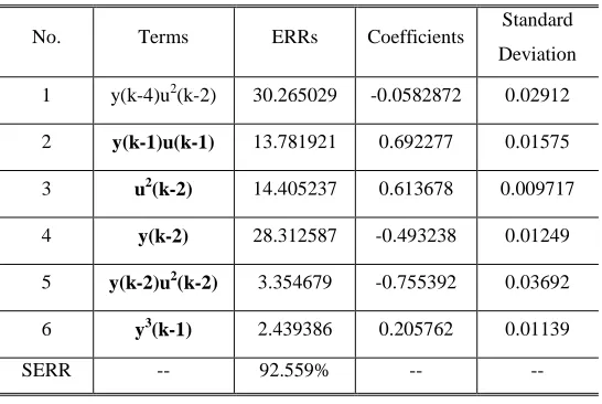
No. Terms ERRs Coefficients Standard Deviation

1 y(k-4)u2(k-2) 30.265029 -0.0582872 0.02912

2 y(k-1)u(k-1) 13.781921 0.692277 0.01575 3 u2(k-2) 14.405237 0.613678 0.009717 4 y(k-2) 28.312587 -0.493238 0.01249 5 y(k-2)u2(k-2) 3.354679 -0.755392 0.03692 6 y3(k-1) 2.439386 0.205762 0.01139 SERR -- 92.559% -- --

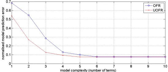
The UOFR was also used to identify the model from the same candidate term dictionary. In the UOFR algorithm, cubic B-spline basis function is used as the modulating function and the first and second order derivatives of the smoothed signals are considered in the ULS criterion. The associated ULS problem in (26) ~ (29) with m=2 is then identified. Table 2 shows the output of the UOFR algorithm. This time the correct term y k

(

−2

)

was selected as the most significant term overwhelming the wrong term

(

) (

2

)

4 2

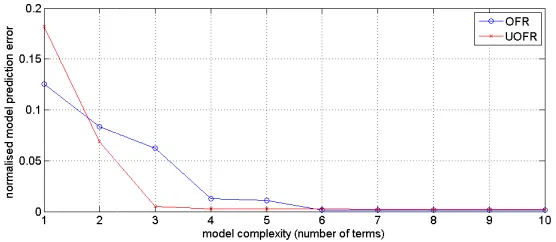
[image:18.595.162.435.154.337.2]

y k− u k− . Under the new ULS criterion, the significance of the redundant term is greatly reduced and does not appear in the model at the UOFR regression process. Figure 2 gives the comparison of the UOFR algorithm and the classic OFR algorithms. The UOFR converged faster than the OFR and obtained the optimal model at the fifth step.

Table 2 Results produced by the UOFR algorithm for example 1

No. Terms ERRs Coefficients Standard Deviation

[image:19.595.160.434.79.197.2]

Figure 2 Compar

5.2 Example 2

Piroddi and Spinelli (2003) has autoregressive terms, even when This is because the time series The “closeness” is represented b product in 2

L space. Hence, whe significant. It will be shown that t ULS criterion is used if it is actuall The example is given as follows

( ) (

( ) ( ) w k u k y k w k

 ₌   =  

where u k

( )

represents the input which is polluted by noise e k

( )

. when the system is persistently algorithm may incorrectly select a components and they recommen poles between 0.75 and 0.9. Rep was generated by the following A

where v k

( )

is Gaussian noise v

coefficient 0.25 is chosen to gua

parison of the UOFR with the classic OFR for exampl

has shown that a classic OFR algorithm may hen the data set was produced from a purely mov

(

)

{

y k−1

}

is always “close” to

{

y k

( )

}

when the s ed by the cross correlation coefficient, which dep when a LS criterion is used, the term y k

(

−1

)

wi hat the significance of the tricky term will be greatly

ually not a correct term.

)

(

)

(

)

( )

3

1

1 0.5 2 0.25 ( 1) ( 2) 0.3 2

1 )

1 0.8

k u k u k u k u k

k e k

z−

− + − + − − − −

+ −

nput signal and y k

( )

represents the observation o . The classic OFR algorithm can correctly detect ently excited. Piroddi and Spinelli has shown tha ect autoregressive terms when the input signal is les mended an input which is generated by an AR pro Repeating Piroddi and Spinelli’s simulation using an ng AR process.

1 2

0.25

( ) ( )

1 1.6 0.64

u k v k

z− z− =

− +

( )

( )

0,1

v k ∼N _{. The AR process has a repeat po}

guarantee the input signal has reasonable amplitu

18 mple 1

ay include redundant moving average model. he sample rate is high. depends on the inner will always be highly atly reduced when the

)

2

(35)

on of the outputw k

( )

the model structure that the classic OFR is less rich in frequency process with two real g an input signal which

(36)

19

( )

e k is a Gaussian distributed noise with a variance 0.02, that is, e k

( )

∼N

(

0, 0.02

)

_{. The results}

produced by the standard OFR algorithm are given in Table 3. Observe that two incorrect autoregressive terms were selected overwhelming the correct terms. A correct term u k

(

−1

) (

u k−2

)

[image:20.595.167.429.199.366.2]

was missed in the identification.

Table 3 Results produced by the standard OFR algorithm for example 2

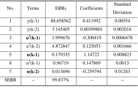
No. Terms ERRs Coefficients Standard Deviation

1 y(k-1) 88.658562 0.411992 0.00554

2 y(k-2) 3.145405 0.00399801 0.002016

3 u3(k-1) 1.999676 -0.300419 0.0006478 4 u3(k-2) 4.872847 0.125053 0.001666

5 u(k-1) 0.179355 1.14722 0.008823 6 u2(k-1) 0.96719 0.147869 0.0013

7 u(k-2) 0.013696 -0.259794 0.01263 SERR -- 99.837% -- --

[image:20.595.157.440.510.631.2]

The output signal and all the candidate terms are modulated using the first and second order derivatives of a cubic B-spline basis function and the UOFR is applied. The identified model by the UOFR is given in Table 4. This time all the correct terms were successfully detected. The redundant terms are avoided using the UOFR algorithm.

Table 4 Model identified using the UOFR algorithm for example 2

No. Terms ERRs Coefficients Standard Deviation

1 u3(k-1) 81.543654 -0.299632 0.0001863 2 u(k-1) 10.684663 1.01012 0.004504 3 u (k-1)u(k-2) 6.937331 0.250064 0.0005112 4 u(k-2) 0.401121 0.490076 0.004161 SERR -- 99.567% -- --

[image:21.595.157.435.135.256.2]

variable y t

( )

in the sense of a caused by y t

( )

−1 .

Figure 3 Compari

5.3 Example 3

This example is also taken from (P selected in the middle of the regr Consider the following system.

( )

0.5 ( ) ( )

w k w

y k w k

 ₌

 

=

 

The system was excited by an inpu

Where v k

( )

is Gaussian noise coefficient 0.16 is chosen so that sequence e k

( )

is a Gaussian dist results produced by the standard terms were selected by the OFR a Table 5 Results pro

No.

a LS criterion. The new UOFR can successfully s

parison of the UOFR with the classic OFR for exampl

(Piroddi & Spinelli, 2003). In this example, the red regression rather than the first step.

(

)

(

)

( )

2 2

1

.5 1 0.8 ( 2) ( 1) 0.05 2 0.5

1 ( )

1 0.5

w k u k u k w k

k e k

z−

− + − + − − − +

+ −

input defined as

1 2

0.16

( ) ( )

1 1.6 0.64

u k v k

z− z− =

− +

ise v k

( )

~N

( )

0,1 . The AR process has a repeat that the input signal has a similar amplitude as v

distributed noise with a variance 0.05, that is, e

ard OFR algorithm are given in Table 5. Observe th FR algorithm at the middle steps of the forward regr s produced by the standard OFR algorithm for examp

Terms ERRs Coefficients Standard Deviation

20 lly solved the problem

mple 2

redundant term is

.5

(37)

(38)

eat pole 0.8 and the

( )

v k . Here the noise

( )

~

(

0, 0.05

)

e k N . The

e that several incorrect regression.

1

2

3 u

4 u(k

5

6 y

7 co

8

SERR

[image:22.595.157.439.70.220.2]

The system was then identified us B-spline basis function were used are given in Table 6. It can be o criterion and detected by the UOF Table 6 Model i

No.

1 u

2

3 y

4 co

5

[image:22.595.160.438.367.499.2]

SERR

Figure 4 shows the comparison of

Figure 4 Compari In all the three examples, the U these benchmark examples which

y(k-1) 90.29322 0.108473 0.001819 y(k-2) 1.888513 0.002894 0.001484

u2(k-1) 1.360357 0.800674 0.002201 (k-1)u(k-2) 3.27943 -0.00893 0.003089

u(k-1) 0.672635 -0.00137 0.002658

y2(k-2) 1.642735 -0.04993 0.000123

constant 0.334417 0.494668 0.001746

u(k-2) 0.487196 -0.79062 0.003265 -- 99.959% -- --

d using the UOFR algorithm. Again the first two deri used to modulate the dependent variable and regr be observed that all the correct terms are significa UOFR algorithm one by one.

del identified using the UOFR algorithm for example

Terms ERRs Coefficients Standard Deviation

u2(k-1) 80.28022 0.79721 0.000443

u(k-2) 10.18902 -0.79724 0.000601

y2(k-2) 7.041134 -0.04997 4.34E-05

constant 2.286183 0.500225 0.000971

y(k-1) 0.127839 0.103086 0.000648 -- 99.924% -- --

n of the OFR and UOFR regression process.

parison of the UOFR with the classic OFR for exampl e UOFR algorithm identified the correct model st hich were deliberately constructed to challenge the

21 derivatives of the cubic regressors. The results nificant under the new

ple 3

mple 3

[image:22.595.156.435.566.685.2]

22 is fair to draw the conclusion that the performance of the new UOFR is significantly improved by applying the new criterion.

6. Conclusions

System identification involves the detection of the model structure and the estimation of the associated parameters under a specific criterion. The drawbacks of the often used least squares criterion have been extensively discussed. Instead of developing a more complex algorithm, a new stricter measurement of the residuals is proposed to improve the system identification performance. The fitness of a model to the weak derivatives of the observed data is combined with the classic least squares criterion to construct a novel ultra least squares criterion. The ULS criterion considers not only the data themselves but also the relations between and amongst the data points. By modifying the m

H norm, the new ULS criterion possesses a clear physical meaning and is easy to implement.

Based on the ULS criterion, a least squares regression problem can be transformed into an associated ultra least squares problem. The ULS criterion characterises the objective model more accurately and the solution space of the ultra least squares problem possesses better properties than that of the original least squares problem. A novel UOFR algorithm was proposed by combining the ULS criterion with the OFR algorithm to efficiently detect the correct model structure. Simulation results shown that the UOFR algorithm significantly improves the performance of the classic OFR algorithm.

In this paper, the ULS criterion has been used for the UOFR algorithm. However, the application of the ULS criterion is not confined to the UOFR algorithm. The ULS criterion can also be used for other optimization methods where the LS criterion has been used.

Acknowledgements

23

References

Ayala Solares, J. R., & Wei, H.-L. (2015). Nonlinear model structure detection and parameter estimation using a novel bagging method based on distance correlation metric. Nonlinear Dynamics, 1-15. doi: 10.1007/s11071-015-2149-3

Baldacchino, T., Anderson, S. R., & Kadirkamanathan, V. Computational system identification for Bayesian NARMAX modelling. Automatica, 49(9), 2641-2651. doi:

http://dx.doi.org/10.1016/j.automatica.2013.05.023

Billings, S. A. (2013). Nonlinear system identification : NARMAX methods in the time, frequency, and spatio-temporal domains. Hoboken, New Jersey: John Wiley & Sons Ltd.

Billings, S. A., & Wei, H. L. (2008). An adaptive orthogonal search algorithm for model subset selection and non-linear system identification. International Journal of Control, 81(5), 714-724. doi: 10.1080/00207170701216311

Bloomfield, P., & Steiger, W. (1980). Least Absolute Deviations Curve-Fitting. SIAM Journal on Scientific and Statistical Computing, 1(2), 290-301. doi: doi:10.1137/0901019

Brewer, D., Barenco, M., Callard, R., Hubank, M., & Stark, J. (2008). Fitting ordinary differential equations to short time course data. Phil. Trans. R. Soc. A, 366(1865), 519-544. doi: 10.1098/rsta.2007.2108

Cormen, T. H., Leiserson, C. E., Rivest, R. L., & Stein, C. (2009). Introduction to Algorithms (3rd ed.). London, England: MIT Press.

Guo, Y., Guo, L. Z., Billings, S. A., & Wei, H. L. (2015). An iterative orthogonal forward regression algorithm. Intern. J. Syst. Sci., 46(5), 776-789. doi: 10.1080/00207721.2014.981237

Kaizhu, H., King, I., & Lyu, M. R. (2008, 15-19 Dec. 2008). Direct Zero-Norm Optimization for Feature Selection. Paper presented at the Data Mining, 2008. ICDM '08. Eighth IEEE International Conference on.

Koza, J. R. (1992). Genetic programming: on the programming of computers by means of natural selection. Cambridge, MA, USA: MIT Press.

Li, K., Peng, J.-X., & Bai, E.-W. (2006). A two-stage algorithm for identification of nonlinear dynamic systems. Automatica, 42(7), 1189-1197. doi:

http://dx.doi.org/10.1016/j.automatica.2006.03.004

Ljung, L. (1987). System Identification: Theory for the User. Englewood Cliffs, N.J.: Prentice-Hall, Inc. Mallat, S. G., & Zhang, Z. (1993). Matching pursuits with time-frequency dictionaries. Signal

Processing, IEEE Transactions on, 41(12), 3397-3415. doi: 10.1109/78.258082

Mao, K. Z., & Billings, S. A. (1997). Algorithms for minimal model structure detection in nonlinear dynamic system identification. International Journal of Control, 68(2), 311-330. doi: 10.1080/002071797223631

Maz'ia, V. G. (1985). Sobolev Space. Berlin; New York: Springer-Verlag.

Narula, S. C., & Wellington, J. F. (1982). The Minimum Sum of Absolute Errors Regression: A State of the Art Survey. International Statistical Review / Revue Internationale de Statistique, 50(3), 317-326. doi: 10.2307/1402501

Piroddi, L., & Spinelli, W. (2003). An identification algorithm for polynomial NARX models based on simulation error minimization. International Journal of Control, 76(17), 1767-1781. doi: 10.1080/00207170310001635419

Preisig, H. A., & Rippin, D. W. T. (1993). Theory and application of the modulating function method - I. Review and theory of the method and theory of the spline-type modulating functions.

Computers & Chemical Engineering, 17(1), 1-16. doi: http://dx.doi.org/10.1016/0098-1354(93)80001-4

Schmidt, M., & Lipson, H. (2009). Distilling Free-Form Natural Laws from Experimental Data. Science, 324(5923), 81-85. doi: 10.1126/science.1165893

24

Appendix A

A set of kth order B-spline basis function can be recursively defined as follows given a set of knots s₀,

1

s , …, s_N, N≥ +k 1.

( )

( )

( )

, , 1 1, 1

1 1

i i k

i k i k i k

i k i i k i

t s s t

B t B t B t

s s s s

+

− + −

+ − + +

− −

= +

− − (39)

with

( )

1

,1

1, 0,

i i

i

s t s

B t otherwise + ≤ <  =

 (40)

The first index indicates the position of the B-spline basis function and the second index denotes the order of the B-spline functions. Using N knots, (N-k) kth order B-spline basis function can be defined. When the knots is uniformly distributed, function Bi k,

( )

t is a time shift of B1,k

( )

t .

The derivative of a k-th order B-spline can be calculated as

( ) ( )

( )

( )

, , 1 1, 1

1 1

1

i k i k i k

i k i i k i

dB t B t B t

k

dt s s s s

− + −

+ − + +

 

= −  − 

− −

  (41)

The higher order derivative of a B-spline basis function can be calculated according to the recursive formula:

( ) ( )

( )

( )

1 , 1 1 , 1

1 1 1, 1

1 1 1 1 r i k r _r i k r r

i k i i k i i k

r

d B t

d B t _dt

k

s s s s

dt d B t