Learning Structural Kernels for Natural Language Processing

Learning Structural Kernels for Natural Language Processing

Department of Computer Science University of Sheffield, United Kingdom

[email protected]

Trevor Cohn

Computing and Information Systems University of Melbourne, Australia

[email protected]

Christian Hardmeier

Department of Linguistics and Philology Uppsala University, Sweden [email protected]

Lucia Specia

Department of Computer Science University of Sheffield, United Kingdom

[email protected]

Abstract

Structural kernels are a flexible learning paradigm that has been widely used in Natural Language Processing. However, the problem of model selection in kernel-based methods is usually overlooked. Previous approaches mostly rely on setting default values for ker-nel hyperparameters or using grid search, which is slow and coarse-grained. In con-trast, Bayesian methods allow efficient model selection by maximizing the evidence on the training data through gradient-based methods. In this paper we show how to perform this in the context of structural kernels by using Gaussian Processes. Experimental results on tree kernels show that this procedure results in better prediction performance compared to hyperparameter optimization via grid search. The framework proposed in this paper can be adapted to other structures besides trees, e.g., strings and graphs, thereby extending the util-ity of kernel-based methods.

1 Introduction

Kernel-based methods are a staple machine learning approach in Natural Language Processing (NLP). Frequentist kernel methods like the Support Vector Machine (SVM) pushed the state of the art in many NLP tasks, especially classification and regression. One interesting aspect of kernels is their ability to be defined directly on structured objects like strings, trees and graphs. This approach has the potential to move the modelling effort from feature engineering to kernel engineering. This is useful when we do not have much prior knowledge about how the data

behaves, as we can more readily define a similarity metric between inputs instead of trying to character-ize which features are the best for the task at hand.

Kernels are a very flexible framework: they can be combined and parameterized in many different ways. Complex kernels, however, lead to the prob-lem ofmodel selection, where the aim is to obtain the best kernel configuration in terms of hyperpa-rameter values. The usual approach for model selec-tion in frequentist methods is to employ grid search on some development data disjoint from the training data. This approach can rapidly become impracti-cal when using complex kernels which increase the number of model hyperparameters. Grid search also requires the user to explicitly set the grid values, making it difficult to fine tune the hyperparameters. Recent advances in model selection tackle some of these issues, but have several limitations (see§6 for details).

Our proposed approach for model selection re-lies on Gaussian Processes (GPs) (Rasmussen and Williams, 2006), a widely used Bayesian kernel ma-chine. GPs allow efficient and fine-grained model selection by maximizing the evidence on the training data using gradient-based methods, dropping the re-quirement for development data. As a Bayesian pro-cedure, GPs also naturally balance between model capacity and generalization. GPs have been shown to achieve state of the art performance in various re-gression tasks (Hensman et al., 2013; Cohn and Spe-cia, 2013). Therefore, we base our approach on this framework.

While prediction performance is important to consider (as we show in our experiments), we are

461

mainly interested in two other significant aspects that are enabled by our approach:

• Gradient-based methods are more efficient than

grid search for high dimensional spaces. This allows us to easily propose new rich kernel ex-tensions that rely on a large number of hyper-parameters, which in turn can result in better modelling capacity.

• Since the model selection process is now

fine-grained, we can interpret the resulting hyperpa-rameter values, depending on how the kernel is defined.

In this work we focus on tree kernels, which have been successfully used in a number of NLP tasks (see§6). In most cases, these kernels are used as an

SVM component and model selection is not consid-ered an important issue. Hyperparameters are usu-ally set to default values, which work reasonably well in terms of prediction performance. However, this is only possible due to the small number of hy-perparameters these kernels contain.

We perform experiments comprising synthetic data (§4) and two real NLP regression tasks: Emo-tion Analysis (§5.1) and Translation Quality

Estima-tion (§5.2). Our findings show that our approach out-performs SVMs using the same kernels.

2 Gaussian Process Regression

Our definition of GPs closely follows that of Rasmussen and Williams (2006). Consider a setting where we have a dataset X =

{(x1, y1),(x2, y2), . . . ,(xn, yn)}, where xi is a d -dimensional input and yi the corresponding out-put. Our goal is to infer an underlying function

f : Rd → Rto explain this data, i.e. f(xi) ≈ yi. Formally,f is drawn from a GP prior,

f(x)∼ GP(µ(x), k(x,x0)),

whereµ(x)is the mean function, which is usually the0constant, andk(x,x0)is thekernelfunction.

In a regression setting, we assume that the res-ponse variables are noisy latent function evaluations, i.e., yi = f(xi) + η, where η ∼ N(0, σ2n) is added white noise. We assume a Gaussian likeli-hood, which allows us to obtain a closed formula

solution for the posterior, namely

y_{∗ ∼ N}(k_∗(K+σnI)−1yT,

k(x_∗,x_∗)₋kT_∗(K+σnI)−1k∗),

where x_∗ and y_∗ are respectively the test input and its response variable, K is the Gram matrix

corresponding to the training inputs and k_∗ = [_hx1,x∗i,hx2,x∗i, . . . ,hxn,x∗i] is the vector of kernel evaluations between the test input and each training input.

A key property of GP models is their ability to perform efficient model selection. This is achieved by employing gradient-based methods to maximize the marginal likelihood,

p(y_|X,θ) =

Z

p(y_|X,θ, f)p(f)df,

whereθrepresents the vector of model hyperparam-eters andyis the vector of response variables from

the training data. For a Gaussian likelihood, we can take the log of the expression above to obtain in closed-form1_,

logp(y_|X,θ) =

−1₂yTG−1y

| {z }

data fit

−1₂log|G_|

| {z }

complexity penalty

−n₂log2π

| {z }

constant

whereG=K+σnI. Thedata fitterm is dependent on the training response variables, while the com-plexity penalty term relies only on the kernel and training inputs. Since the first two terms have con-flicting objectives, optimizing the log marginal like-lihood will naturally achieve a compromise and thus limit overfitting (without the need for any validation step or additional data).

To enable gradient-based optimization we need to derive the gradients w.r.t. the hyperparameters:

∂ ∂θjlog

p(y|X,θ) =1 2y

T_G−1∂G ∂θj

G−1y

−1₂ trace

G−1∂G ∂θj

.

1_{See Rasmussen and Williams (2006, pp. 113-114) for}

The gradients ofGdepend on the underlying ker-nel. Therefore we can employ any kind of valid kernel in this procedure as long as its gradients can be computed. This not only allows for fine-tuning of hyperparameters but also allows for kernel exten-sions which are richly parameterized.

3 Tree Kernels

The seminal work on Convolution Kernels by Haus-sler (1999) defines a broad class of kernels on dis-crete structures by counting and weighting the num-ber of substructures they share. Applying Haussler’s formulation to trees we reach a general formula for a tree kernel between two treest1andt2, namely

k(t1, t2) =

X

f∈F

w(f)c1(f)c2(f), (1)

whereF is the set of all tree fragments, c1(f) and c2(f)return the counts for fragmentfin treest1and t2, respectively, andw(f)assigns a weight to

frag-ment f. In other words, we can consider the

ker-nel a weighted dot product over vectors of fragment counts. The actual fragment set F is deliberately left undefined: different concepts of tree fragments define different tree kernels.

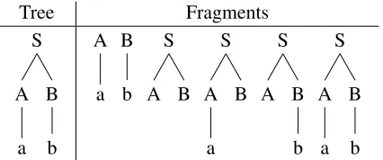
In this paper, we will focus on Subset Tree Ker-nels (henceforth SSTK), first introduced by Collins and Duffy (2001). This kernel considers tree frag-ments that contains complete grammar rules (see Figure 1 for an example). Consider the set of nodes in the two trees asN1 andN2 respectively. We

de-fineIi(n) as an indicator function that returns 1 if fragment fi ∈ F has root n and 0 otherwise. A SSTK can then be defined as:

k(t1, t2) =

X

n1∈N1

X

n2∈N2

∆(n1, n2), (2)

where ∆(n1, n2) =

|F|

X

i=1

λs(2i)I_i(n₁)I_i(n₂)

ands(i)is the number of fragments iniwith at least

one child2_.

The formulation in Equation 2 is the same as the one shown in Equation 1, except that we are now restricting the weights w(f) to be a function of a 2_{See Pighin and Moschitti (2010) for details and a proof on}

this derivation.

Tree Fragments

S

B

b A

a

A

a B

b S

B A

S

B A

a

S

B

b A

S

B

b A

a

Figure 1: An example tree and the respective set of tree fragments defined by a SSTK.

hyperparameterλ. The original goal ofλis to act

as a decay factor that penalizes contributions from larger fragments cf smaller ones (and therefore, it should be in the[0,1]interval). Without this factor, the resulting distribution over tree pairs is skewed, giving extremely large values when trees are equal and rapidly decreasing for small differences over fragment counts. The decay factor helps to spread this distribution, effectively giving smaller weights to larger fragments.

The function∆can be defined recursively,

∆(n1, n2) =

          

0 pr(n1)6=pr(n2) λ pr(n1) =pr(n2)∧

preterm(n1) λg(n1, n2) otherwise,

where pr(n) is the grammar production at node n

and preterm(n) returnstrue ifnis a pre-terminal

node. The functiongis defined as follows:

g(n1, n2) =

|n1|

Y

i=1

(α+ ∆(ci_n1, ci_n2)), (3)

where|n_|is the number of children of noden and ci

nis theithchild of noden. This recursive defini-tion is calculated efficiently by employing dynamic programming to cache intermediate∆results.

Equation 3 also adds another hyperparameter, α.

This hyperparameter was introduced by Moschitti (2006b)3 _{as a way to select between two} differ-ent tree kernels. If α = 1, we get the original SSTK, ifα= 0, then we obtain the Subtree Kernel, which only allows fragments with terminal symbols 3_{In his original formulation, this hyperparameter was named}

as leaves. We can also interpret the Subtree Kernel as a “sparse” version of the SSTK, where the “non-subtree” fragments have their weights equal to zero. Even though fragment weights are affected by both kernel hyperparameters, previous work did not discuss their effects. The usual procedure fixesαto

1(selecting the original SSTK) and sets λto a de-fault value (around0.4). As explained in§2, the GP model selection procedure enables us to learn fine-grained values for these hyperparameters, which can lead to better performing models and aid interpreta-tion. Furthermore, it also allows us to extend these kernels by adding new hyperparameters. We pro-pose one such kernel in the next Section.

3.1 Symbol-aware Subset Tree Kernel

While varying the SSTK hyperparameters can lead to different weight schemes, they do that in a very coarse way. For some applications, it may be nec-essary to give more weight to specific fragments or set of fragments (e.g., NPs being more impor-tant than ADVP in an information extraction set-ting). TheSymbol-aware Subset Tree Kernel (hence-forth, SASSTK), which we introduce here, allows a more fine-grained control over the weights by em-ploying one λ and one α hyperparameter for each non-terminal symbol in the training data. The calcu-lation uses a similar recursive formula to the SSTK, namely:

∆(n1, n2) =

          

0 pr(n1)6=pr(n2) λx pr(n1) =pr(n2)∧

preterm(n1) λxgx(n1, n2) otherwise,

wherexis the symbol at noden1 and

gx(n1, n2) =

|n1|

Y

i=1

(αx+ ∆(cin1, c i

n2)). (4)

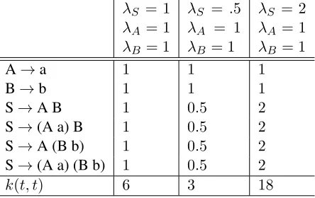
The SASSTK can be interpreted as a generaliza-tion of the SSTK: we can recover the latter by tying allλand setting allα = 1. By employing different hyperparameter values for each specific symbol, we can effectively modify the weights of all fragments where the symbol appears. Table 1 shows an exam-ple where we unrolled a kernel computation into its corresponding feature space, showing the resulting weighted counts for each feature.

λS = 1 λA = 1 λB = 1

λS = .5 λA = 1 λB = 1

λS = 2 λA= 1 λB= 1

A→a 1 1 1

B→b 1 1 1

S→A B 1 0.5 2

S→(A a) B 1 0.5 2

S→A (B b) 1 0.5 2

S→(A a) (B b) 1 0.5 2

k(t, t) 6 3 18

Table 1: Resulting fragment weighted counts for the ker-nel evaluationk(t, t), for different values of

hyperparam-eters, wheretis the tree in Figure 1.

3.2 Kernel Gradients

To enable hyperparameter optimization via gradient descent we must provide gradients for the kernels. In this Section we derive the gradients for SASSTK. From Equation 2 we know that the kernel is a dou-ble summation over the ∆function. Therefore all gradients are also double summations, but over the gradients of∆. We can obtain these in a vectorized way, by considering the gradients of the hyperpa-rameter vectorsλandαover∆. Letkbe the

num-ber of symbols considered in the model andλ and α be k-dimensional vectors containing the

respec-tive hyperparameters.

In the following, we use the notation ∆i as a shorthand for∆(ci_n1, ci_n2)and we also omit the pa-rameters ofgx. We start with theλgradient:

∂∆

∂λ =

            

0 pr(n1)6=pr(n2)

u pr(n1) =pr(n2)∧

preterm(n1) ∂(λxgx)

∂λ otherwise,

wherexis the symbol atn1,gx is defined in Equa-tion 4 andu is thek-dimensional unit vector with the element corresponding to symbolx equal to 1 and all others equal to0. The gradient in the third case is defined recursively,

∂(λxgx)

∂λ =ugx+λx

∂gx ∂λ

=ugx+λx |n1|

X

i=1 gx αx+ ∆i

Theαgradient is derived in a similar way,

∂∆

∂α =

      

0 pr(n1)6=pr(n2)∨

preterm(n1) ∂(λxgx)

∂α otherwise,

and the gradient at the second case is also defined recursively,

∂(λxgx) ∂α =λx

∂gx ∂α

=λx |n1|

X

i=1 gx αx+ ∆i

u+∂∆i

∂α

.

Gradients can be efficiently obtained using dy-namic programming. In fact, they can be calculated at the same time as∆to improve performance since they all share many terms in their derivations. Fi-nally, we can easily obtain the gradients for the orig-inal SSTK by lettingu= 1.

3.3 Kernel Normalization

It is common practice when using tree kernels to nor-malize the kernel. This helps reduce the random ef-fect of tree size. Normalization can be achieved us-ing the followus-ing, where_kˆ_{is the normalized kernel:}

ˆ

k(t1, t2) =

k(t1, t2)

p

k(t1, t1)k(t2, t2) .

To apply this normalized version in the optimiza-tion procedure we must also derive gradients for the normalization function. In the following equation, we usekij andkˆij as a shorthand for k(ti, tj) and

ˆ

k(ti, tj), respectively:

∂kˆ12 ∂θ =

∂k12 ∂θ

√

k11k22 −

ˆ

k12 ∂k11

∂θ k22+k11

∂k22 ∂θ 2k11k22

.

3.4 Other Extensions

Many other structural kernels rely on recursive def-initions and dynamic programming to perform their calculations. Examples include other tree kernels like the Partial Tree Kernel (Moschitti, 2006a) and string kernels like the ones defined on character n-grams (Lodhi et al., 2002) or word sequences (Can-cedda et al., 2003). While in this paper we focus

on the SSTK (and our proposed SASSTK), our ap-proach can easily be extended to these other kernels, as long as all the corresponding recursive definitions are differentiable.

4 Synthetic Data Experiments

A natural question that arises in the proposed method is how much data is needed to accurately learn the kernel hyperparameters. To answer this question, we run a set of experiments using synthetic data. We generate this data by using a set of1000 natural language syntactic trees, where we fix a ran-dom subset of200instances for testing and use the remaining800instances as training. For each train-ing set size we define a GP over the full dataset, sam-ple a function from it and use the function output as the response variable for each tree. We try two dif-ferent GP priors, one using the SSTK and another one using the SASSTK.

The conditions above provide a controlled envi-ronment to check the modelling capacities of our ap-proach since we know the exact distribution where the data comes from. The reasoning behind these experiments is that to be able to provide benefits in real tasks, where the data distribution is not known, our models have to be learnable in this controlled setting as well using a reasonable amount of data.

Finally, we also provide an empirical evaluation comparing the speed performance between our ap-proach and grid search.

4.1 SSTK Prior

Our first experiments use a SSTK as the kernel with

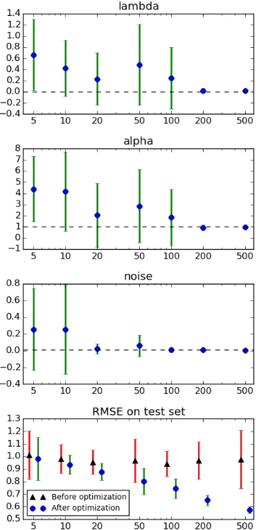
Figure 2 shows the results of these experiments. For small sizes the variance in the resulting hyperpa-rameter values is large but as soon as we reach200 instances we are able to retrieve the original values with high confidence. In other words, in an ideal set-ting200instances are enough to learn the kernel. It is also interesting to note that test RMSE after opti-mization steadily decreases as we increase training data size. This shows that if one is more interested in predictions themselves, it is still worth optimizing hyperparameters even if the training data is small.

Figure 2: Results of synthetic experiments optimizing SSTK. The x axes correspond to different training set

sizes and the they axes are the obtained hyperparame-ter values in the first three plots and RMSE in the last plot. Dashed lines show the original hyperparameter val-ues. Points are offset in RMSE chart for legibility.

4.2 SASSTK Prior

The large number of hyperparameters of the SASSTK makes it more prone to optimization and overfitting issues when compared to the SSTK. This raises the question of how much data is needed to justify its use. To address this question, we run sim-ilar experiments to those above for the SSTK, except that now we sample from a GP using a SASSTK as the kernel.

Instead of optimizing all hyperparameters freely we use a simpler version where we tieλandα for

each symbol to the same value, except for the sym-bol ’S’. Effectively this version has one extraλand one extraα(henceforthλSandαS) when compared to the SSTK. The GP prior hyperparameter values are set toλ = 0.001, λS = 0.5, α = 0.1, αS = 1 andσ2_n = 0.01. For each training set size, we train two GPs, one using this SASSTK and one using the original SSTK, optimize them using10random restarts and measure RMSE on the test set.

Results are shown in Figure 3. For all training set sizes the SASSTK reaches lower RMSE than SSTK, with a substantial difference after reaching 100 in-stances. This shows that even for small datasets our proposed kernel manages to capture aspects which can not be explained by the original SSTK. Note that this is an ideal setting, and real datasets may need to be larger to realize gains from SASSTK. Neverthe-less, these are promising results since they give evi-dence of a small lower bound on the dataset size for SASSTK to be effective.

Figure 3: Results from synthetic experiments comparing SSTK and SASSTK. Thexaxis is training set size while

4.3 Performance Experiments

To provide an overview of how efficient is the gradient-based method compared to grid search we also run a set of experiments measuring wall clock training time vs. RMSE on a test set. For both GP and SVM models we employ the SSTK as the kernel and we use the same synthetic data from the previ-ous experiments4_{. We perform20runs, keeping the} test set as the same 200 instances for all runs and randomly sampling200instances from the remain-ing instances as trainremain-ing data.

Figure 4 shows the curves for both GP and SVM models. The GP curve is obtained by increasing the maximum number of iterations of the gradient-based method (in this case, L-BFGS) and the SVM curve is obtained by increasing the granularity of the grid size.

Figure 4: Results from performance experiments. Thex

axis corresponds to wall clock time in seconds and it is in log scale. Theyaxis shows RMSE on the test set. The

blue dashed line corresponds to the RMSE value obtained after L-BFGS converged. Error bars are obtained by mea-suring one standard deviation over the20runs made in each experiment.

We can see that optimizing the GP model is con-sistently much faster than doing grid search on the SVM model (notice the logarithmic scale), even though it shows some variance when letting L-BFGS run for a larger number of iterations. The GP model also is able to better predictions in general. Even when taking the variances into account, grid search would still need around10times more computation 4_{For specific details on the SVM models used in all}

experi-ments performed in this paper we refer the reader to Appendix A.

time to achieve the same predictions obtained by the GP model. In real settings, SVMs predictions tend to be more on par with the ones provided by a GP (as shown in§5) but nevertheless these figures show that the GP can be much more time efficient when optimizing hyperparameters of a tree kernel.

An important performance aspect to take into ac-count is parallelization. Grid search is embarass-ingly parallelizable since each grid point can run in a different core. However, the GP optimization can also benefit from multiple cores by running each ker-nel computation inside the Gram matrix in parallel. To keep the comparisons simpler, the results shown in this section use a single core but all experiments in

§5 employ parallelization in the Gram matrix com-putation level (for both SVM and GP models).

5 NLP Experiments

Our experiments with NLP data address two regres-sion tasks: Emotion Analysis and Quality Estima-tion. For both tasks, we use the Stanford parser (Manning et al., 2014) to obtain constituency trees for all sentences. Also, rather than using data official splits, we perform 5-fold cross-validation in order to obtain more reliable results.

5.1 Emotion Analysis

The goal of Emotion Analysis is to automatically de-tect emotions in a text (Strapparava and Mihalcea, 2008). This problem is closely related to Opinion Mining (Pang and Lee, 2008), with similar appli-cations, but it is usually done at a more fine-grained level and involves the prediction of a set of labels for each text (one for each emotion) instead of a single label.

Beck et al. (2014a) used a multi-task GP for this task with a bag-of-words feature representation. In theory, it is possible to combine their multi-task ker-nel with our tree kerker-nels, but to keep the focus of the experiments on testing tree kernel approaches, here we use independently trained models, one per emo-tion.

Sur-prise. For each emotion, a score between0and100 is given, 0meaning total lack of emotion and 100, maximally emotional. Scores are mean-normalized before training the models.

Models We perform experiments using the follow-ing tree kernels:

• SSTK: the SSTK formulation introduced by

Moschitti (2006b);

• SASSTKfull: our proposed Symbol-Aware SSTK;

• SASSTKS:same as before, but using only two

λ and two α hyperparameters: one for

sym-bols corresponding to full sentences5 _and an-other for all an-other symbols. This configuration is similar to that in Section 4.2.

For all kernels, we also use a variation fixing theα

hyperparameters to1to emulate the original SSTK. Baselines and evaluation Our results are com-pared against three baselines:

• SVM SSTK:a SVM using an SSTK kernel.

• SVM BOW:same as before, but using an RBF kernel with a bag-of-words representation.

• GP BOW:same as SVM BOW but using a GP

instead.

The SVM models are trained using a wrapper for LIBSVM6 _{(Chang and Lin, 2001) provided by the} scikit-learn toolkit7_{(Pedregosa et al., 2011) and} op-timized via grid search. Following previous work, we use Pearson’s correlation coefficient as evalua-tion metric. Pearson’s scores are obtained by con-catenating all six emotions outputs together.

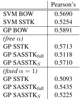
Table 2 shows the results. The best GP model with tree kernels outperforms the SVMs, showing that the fine-grained model selection procedure pro-vided by the GP models is helpful when dealing with tree kernels. However, using the SASSTK models do not help in the case of freeαand the SASSTKfull actually performs worse than the original SSTK, 5_{In this dataset, symbols areS,SQ,SBARQandSIN V.}

6_{http://www.csie.ntu.edu.tw/˜cjlin/}

libsvm

7_{http://scikit-learn.org}

even though the optimized marginal likelihood was higher. This is evidence that the SASSTKfullmodel is overfitting the training data, probably due to its large number of hyperparameters.

Pearson’s

SVM BOW 0.5690

SVM SSTK 0.5254

GP BOW 0.5891

(freeα)

GP SSTK 0.5713

GP SASSTKfull 0.5118 GP SASSTKS 0.5710 (fixedα = 1)

GP SSTK 0.5093

GP SASSTKfull 0.5435 GP SASSTKS 0.5225

Table 2: Pearson’s correlation scores for the Emotion Analysis task (higher is better).

Another interesting finding in Table 2 is that fix-ing theαvalues often harms performance.

Inspect-ing the freeα models showed that the values found

by the optimizer were very close to zero. This in-dicates that the model selection procedure prefer towards giving smaller weights to incomplete tree fragments. We can interpret this as the model se-lecting a more lexicalized feature space, which also explains why the GP RBF model on bag-of-words performed the best in this task.

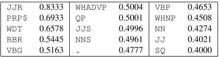
Finally, to understand how the optimized kernels could provide more interpretability, Table 3 shows the top 15 λ values obtained by the SASSTKfull (fixedαvariant) with their corresponding symbols.

In this specific case the kernel does not give the best performance so there are limitations in doing a full linguistic analysis. Nevertheless, we believe this ex-ample shows the potential for developing more in-terpretable kernels. This is especially interesting be-cause these models take into account a much richer feature space than what it is allowed by parametric models.

5.2 Quality Estimation

Exam-JJR 0.8333 WHADVP 0.5004 VBP 0.4653

PRP$ 0.6933 QP 0.5001 WHNP 0.4508

WDT 0.6578 JJS 0.4996 NN 0.4274

RBR 0.5445 NNS 0.4961 JJ 0.4021

VBG 0.5163 . 0.4777 SQ 0.4000

Table 3: Top 15 symbols sorted according to their ob-tainedλvalues in the SASSTKfull model with fixedα.

The numbers are the corresponding λvalues, averaged

over all six emotions.

ples of applications include filtering machine trans-lated sentences that would require more post-editing effort than translation from scratch (Specia et al., 2009), selecting the best translation from different MT systems (Specia et al., 2010) or between an MT system and a translation memory (He et al., 2010), and highlighting segments that need revision (Bach et al., 2011). While various quality metrics exist, here we focus onpost-editing timeprediction.

Tree kernels have been used before in this task (with SVMs) by Hardmeier (2011) and Hardmeier et al. (2012). While their best models combine tree kernels with a set of explicit features, they also show good results using only the tree kernels. This makes Quality Estimation a good benchmark task to test our models.

Datasets We use two publicly available datasets containing post-edited machine translated sentences. Both are composed of a set of source sentences, their machine translated outputs and the corresponding post-editing time.

• French-English (fr-en): This dataset,

de-scribed in (Specia, 2011), contains2524French sentences translated into English and post-edited by a novice translator.

• English-Spanish (en-es): This dataset was used in the WMT14 Quality Estimation shared task (Bojar et al., 2014), containing 858 sen-tences translated from English into Spanish and post-edited by an expert translator.

For each dataset, post-editing times are first di-vided by the translation output length (obtaining the post-editing time per word) and then mean normal-ized.

Models Since our data consists of pairs of trees, our models in this task use a pair of tree kernels. We combine these two kernels by either summing or multiplying them. As for underlying tree ker-nels, we try both SSTK and SASSTKS. As in the Emotion Analysis task, we also experiment with a set of kernel configurations with theα hyperparam-eters fixed at 1. We also test models that combine our tree kernels with an RBF kernel on a set of17 features extracted using the QuEst framework (Spe-cia et al., 2013). These features are part of a strong baseline model used by the WMT14 shared task. Baselines and evaluation We compare our results with a number of SVM models:

• SVM SSTK:same as in the Emotion Analysis

task, using either a sum (+) or a product (×) of SSTKs.

• SVM RBF:this is an SVM trained on the 17 features extracted by Quest.

• SVM RBF SSTK: a combination of the two models above.

For further comparison, we also show results ob-tained using a GP model and an RBF kernel on the QuEst-only features. Following previous work, we measure prediction performance using both Mean Absolute Error (MAE) and RMSE.

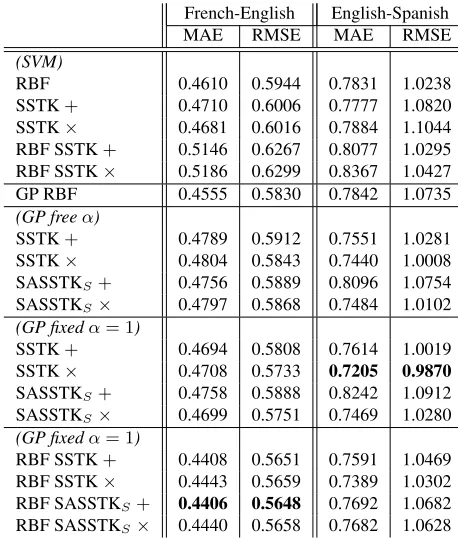
The prediction results are given in Table 4. They indicate a number of interesting findings:

• For thefr-endataset, the GP models combining tree kernels with an RBF kernel outperform all other models. Results for theen-esdataset are less consistent, probably due to the small size of the dataset, but on average they are better than their SVM counterparts.

• Unlike in the Emotion Analysis task, fixingα

results in better performance, even though the resulting models have lower marginal likeli-hood than the ones with freeα. The same effect happened when comparing the SASSTK mod-els with the SSTK ones for theen-es dataset. Both cases are evidence of model overfitting.

French-English English-Spanish MAE RMSE MAE RMSE

(SVM)

RBF 0.4610 0.5944 0.7831 1.0238 SSTK+ 0.4710 0.6006 0.7777 1.0820 SSTK× 0.4681 0.6016 0.7884 1.1044 RBF SSTK+ 0.5146 0.6267 0.8077 1.0295 RBF SSTK× 0.5186 0.6299 0.8367 1.0427 GP RBF 0.4555 0.5830 0.7842 1.0735

(GP freeα)

SSTK+ 0.4789 0.5912 0.7551 1.0281 SSTK× 0.4804 0.5843 0.7440 1.0008 SASSTKS+ 0.4756 0.5889 0.8096 1.0754

SASSTKS× 0.4797 0.5868 0.7484 1.0102 (GP fixedα= 1)

SSTK+ 0.4694 0.5808 0.7614 1.0019 SSTK× 0.4708 0.5733 0.7205 0.9870 SASSTKS+ 0.4758 0.5888 0.8242 1.0912

SASSTKS× 0.4699 0.5751 0.7469 1.0280 (GP fixedα= 1)

RBF SSTK+ 0.4408 0.5651 0.7591 1.0469 RBF SSTK× 0.4443 0.5659 0.7389 1.0302 RBF SASSTKS+ 0.4406 0.5648 0.7692 1.0682

RBF SASSTKS× 0.4440 0.5658 0.7682 1.0628

Table 4: Error scores for the Quality Estimation task (lower is better). Results are in terms of post-editing time per word. Bold scores are the best ones for each dataset.

We also inspect the resulting hyperparameters to obtain insights about the features used by the model. Table 5 shows the optimized λ values for the GP

SSTK models with fixedαfor thefr-endataset. The λvalues obtained are higher for the target sentence

kernels than for the source sentence ones. We can interpret this as the model giving preference to fea-tures from the target trees instead of the source trees, which is what we would expect for this task. 5.3 Overfitting

Both NLP tasks show evidence that the GP models with large number of hyperparameters (SASSTKfull in the case of Emotion Analysis and the freeα

mod-els in Quality Estimation) are overfitting the cor-responding datasets. While the Bayesian

formula-λsrc λtgt GP SSTK+ 0.1394 0.3108 GP SSTK× 0.1405 0.2641

Table 5: Learned hyperparameters for the GP SSTK mod-els in thefr-endataset, withαfixed at1. λsrcandλtgt are the hyperparameters corresponding to the kernels on the source and target parse trees, respectively. The values shown are averaged over the cross-validation results.

tion for the marginal likelihood does help limiting overfitting, it does not prevent it completely. Small datasets or invalid assumptions about the Gaussian distribution of the data may still lead to poorly fitting models. Another means of reducing overfitting is by taking a fully Bayesian approach in which hyperpa-rameters are considered as random variables and are marginalized out (Osborne, 2010); this is a research direction we plan to pursue in the future.8

5.4 Extensions to Other Tasks

The GP framework introduced in Section 2 can be extended to non-regression problems by chang-ing the likelihood function. For instance, models for classification (Rasmussen and Williams, 2006, Chap. 3), ordinal regression (Chu and Ghahramani, 2005) and structured prediction (Altun et al., 2004; Brati`eres et al., 2013) were proposed in the liter-ature. Since the likelihood is independent of the kernel, a natural future step is to apply the kernels and models introduced in this paper to different NLP tasks.

In light of that, we did initial experiments with constituency parsing reranking.9 _{The first results} were inconclusive but we do believe this is because we employed naive approaches using classification (1-best result vs. all) and regression (using PARSE-VAL metrics as the response variable) models. A more appropriate way to tackle this task is by em-ploying a reranking-based likelihood and this is a direction we plan to pursue in the future.

6 Related Work

Interest in model selection procedures for kernel-based methods has been growing in the last years. 8_{See also Rasmussen and Williams (2006, Chap. 5) for an}

in-depth discussion on this issue.

One widely used approach for that is Multiple Ker-nel Learning (MKL) (G¨onen and Alpaydın, 2011). MKL is based on the idea of using combinations of kernels to model the data and developing algo-rithms to tune the kernel coefficients. This is dif-ferent from our method, where we focus on learning the hyperparameters of a single structural kernel. An approach similar to ours was proposed by Igel et al. (2007). They combine oligo kernels (a kind of n-gram kernel) with MKL, derive their gradients and optimize towards a kernel alignment metric. Com-pared to our approach, they restrict the length of the n-grams being considered, while we rely on dy-namic programming to explore the whole substruc-ture space. Also, their method does not take into account the underlying learning algorithm. Another recent approach proposed for model selection is ran-dom search (Bergstra and Bengio, 2012). Like grid search, it has the drawback of not employing gra-dient information, as it is designed for any kind of hyperparameters (including categorical ones).

Structural kernels have been successfully em-ployed in a number of NLP tasks. The original SSTK proposed by Collins and Duffy (2001) was used to rerank the output of syntactic parsers. Re-cently, this reranking idea was also applied to dis-course parsing (Joty and Moschitti, 2014). Other tree kernel applications include Semantic Role La-belling (Moschitti et al., 2008) and Relation Extrac-tion (Plank and Moschitti, 2013). String kernels were mostly used in Text Classification (Lodhi et al., 2002; Cancedda et al., 2003), while graph ker-nels have been used for recognizing Textual Entail-ment (Zanzotto and Dell’Arciprete, 2009). How-ever, these previous works focused on frequentist methods like SVM or voted perceptron while we employ a Bayesian approach.

Gaussian Processes are a major framework in machine learning nowadays: applications in-clude Robotics (Ko et al., 2007), Geolocation (Schwaighofer et al., 2004) and Computer Vision (Sinz et al., 2004). Only very recently they have been successfully employed in a few NLP tasks such as translation quality estimation (Cohn and Specia, 2013; Beck et al., 2014b), detection of temporal pat-terns in text (Preot¸iuc-Pietro and Cohn, 2013), se-mantic similarity (Rios and Specia, 2014) and emo-tion analysis (Beck et al., 2014a). In terms of feature

representations, previous work focused on the vecto-rial inputs and applied well-known kernels for these inputs, e.g. the RBF kernel. As shown on§5.2, our

approach is orthogonal to these previous ones, since kernels can be easily combined in different ways.

It is important to note that we are not the first ones to combine GPs with kernels on structured inputs. Driessens et al. (2006) employed a combination of GPs and graph kernels for reinforcement learning. However, unlike our approach, they did not attempt model selection, evaluating only a few hyperparam-eter values empirically.

7 Conclusions

This paper describes a Bayesian approach for struc-tural kernel learning, based on Gaussian Processes for easy model selection. Experiments applying our models to synthetic data showed that it is possible to learn structural kernel hyperparameters using a fairly small amount of data. Furthermore we ob-tained promising results in two NLP tasks, includ-ing Quality Estimation, where we beat the state of the art. Finally, we showed how these rich parame-terizations can lead to more interpretable kernels.

Beyond empirical improvements, an important goal of this paper is to present a method that en-ables new kernel developments through the exten-sion of the number of hyperparameters. We focused on the Subset Tree Kernel, proposing an extension and then deriving its gradients. This approach can be applied to any structural kernel, as long as gradi-ents are available. It is our hope that this work will serve as a starting point for future developments in these research directions.

Acknowledgements

Daniel Beck was supported by funding from CNPq/Brazil (No. 237999/2012-9). Dr. Cohn is the recipient of an Australian Research Council Future Fellowship (project number FT130101105). The au-thors would also like to thank the three anonymous reviewers for their helpful comments and sugges-tions.

References

Segmenting and Annotating Sequences. In Proceed-ings of ICML.

Nguyen Bach, Fei Huang, and Yaser Al-Onaizan. 2011. Goodness: A Method for Measuring Machine Trans-lation Confidence. InProceedings of ACL, pages 211– 219.

Daniel Beck, Trevor Cohn, and Lucia Specia. 2014a. Joint Emotion Analysis via Multi-task Gaussian Pro-cesses. InProceedings of EMNLP, pages 1798–1803. Daniel Beck, Kashif Shah, and Lucia Specia. 2014b.

SHEF-Lite 2.0 : Sparse Multi-task Gaussian Processes for Translation Quality Estimation. InProceedings of WMT14, pages 307–312.

James Bergstra and Yoshua Bengio. 2012. Random Search for Hyper-Parameter Optimization. Journal of Machine Learning Research, 13:281–305.

John Blatz, Erin Fitzgerald, and George Foster. 2004. Confidence estimation for machine translation. In Proceedings of the 20th Conference on Computational Linguistics, pages 315–321.

Ondej Bojar, Christian Buck, Christian Federmann, Barry Haddow, Philipp Koehn, Johannes Leveling, Christof Monz, Pavel Pecina, Matt Post, Herve Saint-amand, Radu Soricut, Lucia Specia, and Aleˇs Tam-chyna. 2014. Findings of the 2014 Workshop on Statistical Machine Translation. In Proceedings of WMT14, pages 12–58.

S´ebastien Brati`eres, Novi Quadrianto, and Zoubin Ghahramani. 2013. Bayesian Structured Prediction using Gaussian Processes.arXiv:1307.3846, pages 1– 17.

Nicola Cancedda, Eric Gaussier, Cyril Goutte, and Jean-Michel Renders. 2003. Word-Sequence Kernels. The Journal of Machine Learning Research, 3:1059–1082. Chih-Chung Chang and Chih-Jen Lin. 2001. LIBSVM : A Library for Support Vector Machines. ACM Trans-actions on Intelligent Systems and Technology (TIST), 2(3):1–39.

Wei Chu and Zoubin Ghahramani. 2005. Gaussian Pro-cesses for Ordinal Regression. Journal of Machine Learning Research, 6:1019–1041.

Trevor Cohn and Lucia Specia. 2013. Modelling Anno-tator Bias with Multi-task Gaussian Processes: An Ap-plication to Machine Translation Quality Estimation. InProceedings of ACL, pages 32–42.

Michael Collins and Nigel Duffy. 2001. Convolution Kernels for Natural Language. In Proceedings of NIPS, pages 625–632.

Kurt Driessens, Jan Ramon, and Thomas G¨artner. 2006. Graph Kernels and Gaussian Processes for Relational Reinforcement Learning. Machine Learning, 64(1-3):91–119.

Mehmet G¨onen and Ethem Alpaydın. 2011. Multi-ple kernel learning algorithms. Journal of Machine Learning Research, 12:2211–2268.

Christian Hardmeier, Joakim Nivre, and J¨org Tiedemann. 2012. Tree Kernels for Machine Translation Quality Estimation. In Proceedings of WMT12, pages 109– 113.

Christian Hardmeier. 2011. Improving Machine Trans-lation Quality Prediction with Syntactic Tree Kernels. InProceedings of EAMT, pages 233–240.

David Haussler. 1999. Convolution Kernels on Discrete Structures. Technical report, University of California at Santa Cruz.

Yifan He, Yanjun Ma, Josef van Genabith, and Andy Way. 2010. Bridging SMT and TM with Translation Recommendation. InProceedings of ACL, pages 622– 630.

James Hensman, Nicol`o Fusi, and Neil D. Lawrence. 2013. Gaussian Processes for Big Data. In Proceed-ings of UAI, pages 282–290.

Christian Igel, Tobias Glasmachers, Britta Mersch, and Nico Pfeifer. 2007. Gradient-based Optimization of Kernel-Target Alignment for Sequence Kernels Ap-plied to Bacterial Gene Start Detection. IEEE/ACM Transactions on Computational Biology and Bioinfor-matics, 4(2):216–226.

Shafiq Joty and Alessandro Moschitti. 2014. Discrimi-native Reranking of Discourse Parses Using Tree Ker-nels. InEMNLP, pages 2049–2060.

Jonathan Ko, Daniel J. Klein, Dieter Fox, and Dirk Haehnel. 2007. Gaussian Processes and Reinforce-ment Learning for Identification and Control of an Au-tonomous Blimp. In Proceedings of IEEE Interna-tional Conference on Robotics and Automation, pages 742–747.

Huma Lodhi, Craig Saunders, John Shawe-Taylor, Nello Cristianini, and Chris Watkins. 2002. Text Classifi-cation using String Kernels. The Journal of Machine Learning Research, 2:419–444.

Christopher D. Manning, Mihai Surdeanu, John Bauer, Jenny Finkel, Steven J. Bethard, and David McClosky. 2014. The Stanford CoreNLP Natural Language Pro-cessing Toolkit. InProceedings of ACL Demo Session, pages 55–60.

Alessandro Moschitti, Daniele Pighin, and Roberto Basili. 2008. Tree Kernels for Semantic Role Label-ing.Computational Linguistics, pages 1–32.

Alessandro Moschitti. 2006a. Efficient Convolution Ker-nels for Dependency and Constituent Syntactic Trees. InProceedings of ECML, pages 318–329.

Michael Osborne. 2010. Bayesian Gaussian Processes for Sequential Prediction, Optimisation and Quadra-ture. Ph.D. thesis, University of Oxford.

Bo Pang and Lillian Lee. 2008. Opinion Mining and Sentiment Analysis. Foundations and Trends in Infor-mation Retrieval, 2(12):1–135.

Fabian Pedregosa, Ga¨el Varoquaux, Alexandre Gram-fort, Vincent Michel, Bertrand Thirion, Olivier Grisel, Mathieu Blondel, Peter Prettenhofer, Ron Weiss, Vin-cent Duborg, Jake Vanderplas, Alexandre Passos, David Cournapeau, Matthieu Brucher, Matthieu Per-rot, and ´Edouard Duchesnay. 2011. Scikit-learn: Ma-chine learning in Python. Journal of Machine Learn-ing Research, 12:2825–2830.

Daniele Pighin and Alessandro Moschitti. 2010. On Re-verse Feature Engineering of Syntactic Tree Kernels. InProceedings of CONLL, pages 223–233.

Barbara Plank and Alessandro Moschitti. 2013. Embed-ding Semantic Similarity in Tree Kernels for Domain Adaptation of Relation Extraction. InProceedings of ACL, pages 1498–1507.

Daniel Preot¸iuc-Pietro and Trevor Cohn. 2013. A tem-poral model of text periodicities using Gaussian Pro-cesses. InProceedings of EMNLP, pages 977–988. Carl Edward Rasmussen and Christopher K. I. Williams.

2006. Gaussian processes for machine learning, vol-ume 1. MIT Press Cambridge.

Miguel Rios and Lucia Specia. 2014. UoW : Multi-task Learning Gaussian Process for Semantic Textual Sim-ilarity. InProceedings of SemEval, pages 779–784. Anton Schwaighofer, Marian Grigoras, Volker Tresp, and

Clemens Hoffmann. 2004. GPPS: A Gaussian Pro-cess Positioning System for Cellular Networks. In Proceedings of NIPS, pages 579–586.

Fabian H. Sinz, Joaquin Qui˜nonero Candela, G¨okhan H. Bakır, Carl E. Rasmussen, and Matthias O. Franz. 2004. Learning Depth from Stereo. Pattern Recog-nition, pages 1–8.

Lucia Specia, Nicola Cancedda, Marc Dymetman, Marco Turchi, and Nello Cristianini. 2009. Estimating the sentence-level quality of machine translation systems. InProceedings of EAMT, pages 28–35.

Lucia Specia, Dhwaj Raj, and Marco Turchi. 2010. Ma-chine translation evaluation versus quality estimation. Machine Translation, 24(1):39–50.

Lucia Specia, Kashif Shah, Jos´e G. C. De Souza, and Trevor Cohn. 2013. QuEst - A translation quality estimation framework. InProceedings of ACL Demo Session, pages 79–84.

Lucia Specia. 2011. Exploiting Objective Annotations for Measuring Translation Post-editing Effort. In Pro-ceedings of EAMT, pages 73–80.

Carlo Strapparava and Rada Mihalcea. 2007. SemEval-2007 Task 14 : Affective Text. InProceedings of Se-mEval, pages 70–74.

Carlo Strapparava and Rada Mihalcea. 2008. Learning to identify emotions in text. InProceedings of the 2008 ACM Symposium on Applied Computing, pages 1556– 1560.

Fabio Massimo Zanzotto and Lorenzo Dell’Arciprete. 2009. Efficient kernels for sentence pair classification. InProceedings of EMNLP, pages 91–100.

A Details on SVM Baselines

All SVM baselines employ the -insensitve loss

function. Grid search optimization is done via 3-fold cross-validation on the respective training set and use RMSE as the metric to be minimized. After obtained the best hyperparameter values, the SVM is retrained using these values on the full respec-tive training set. The specific intervals used in grid search depend on the task.

For the performance experiments on synthetic data, we employed an interval of [10−2_{,10] for C}

(regularization coefficient) and,[10−8,1]forλand

[10−4,2] for α. In each run we incrementally

in-crease the size of the grid by adding intermediate values on each interval. We keep a linear scale for the SSTK hyperparameters and a logarithmic scale forC and. As an example, Table 6 shows the

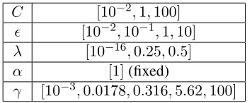
re-sulting grids when the grid value is4for each hyper-parameter. For all NLP experiments the grid is fixed for all hyperparameters (includingγ, the lengthscale

value in the RBF kernel), with its corresponding val-ues shown on Table 7.

C/ [10−2,10−1,1,10]

λ [10−8,0.33,0.67,1]

α [10−4,0.67,1.33,2]

Table 6: Resulting grids for the performance experiments when grid size is set to4for each hyperparameter.

C [10−2,1,100]

[10−2,10−1,1,10]

λ [10−16,0.25,0.5]

α [1](fixed)

γ [10−3,0.0178,0.316,5.62,100]