Three dimensional thermal-solute phase field simulation of binary alloy solidification

Contents lists available atScienceDirect

Journal

of

Computational

Physics

www.elsevier.com/locate/jcp

Three

dimensional

thermal-solute

phase

field

simulation

of binary

alloy

solidification

P.C. Bollada

a,

∗

,

C.E. Goodyer

a,b

,

P.K. Jimack

a

,

A.M. Mullis

a

,

F.W. Yang

a a_{University of Leeds, United Kingdom}

b_{Numerical Algorithms Group, United Kingdom}

a

r

t

i

c

l

e

i

n

f

o

a

b

s

t

r

a

c

t

Article history:

Received8September2014

Receivedinrevisedform20January2015 Accepted28January2015

Availableonline3February2015

Keywords:

Phasefield Dendrite Solidification Adaptivemesh Multigrid NonlinearPDEs

Weemployadaptivemeshrefinement,implicittimestepping,anonlinearmultigridsolver and parallel computation to solve a multi-scale, time dependent, three dimensional, nonlinearsetofcoupledpartial differentialequationsforthreescalarfieldvariables.The mathematicalmodel represents thenon-isothermalsolidification ofametal alloyintoa meltsubstantiallycooledbelow itsfreezingpoint atthe microscale.Underlyingphysical molecular forces are captured at this scale by a specification ofthe energy field. The time rate of change of the temperature, alloy concentration and an order parameter to govern the state of the material (liquid or solid) are controlled by the diffusion parametersand variationalderivativesofthe energyfunctional.The physical problemis importanttomaterialscientists forthe developmentofsolidmetal alloys and,hitherto, thisfully coupledthermalproblem hasnotbeen simulated inthreedimensions,dueto its computationally demanding nature. By bringing together stateof the art numerical techniquesthisproblemisnowshownheretobetractableatappropriateresolutionwith relativelymoderatecomputationalresources.

©2015TheAuthors.PublishedbyElsevierInc.ThisisanopenaccessarticleundertheCC BYlicense(http://creativecommons.org/licenses/by/4.0/).

1. Introduction

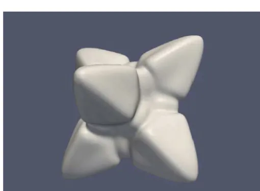
We herepresentourcomputationalapproachtosimulating,atthemeso-scale,threedimensional,non-isothermalalloy solidification froman initial small, sphericalseed into a mature, dendriticcrystal. A feature of amature dendrite is the geometriccomplexityofitsevolvingtwo-dimensionalsurface(seeFig. 1foratypicalsnapshotintime).Thismakestracking of thesurface a difficult taskinsharpinterface models. Aphase-fieldmodel avoidsthisby making useof aphase field,

φ (

x

,

t

)

∈ [−

1

,

1

]

, torepresent, atits two extremes,the liquidandsolid state respectivelyandthe evolutionof thephase boundary,

φ

=

0,isthesurfaceofinterest.Thissolvesoneproblem,butatacostofintroducinganother.Thecomputation requiresan extravariable,thephase,whichvariesrapidlyoverasmallregionabouttheinterface.Takingthethicknessof theinterfacetobe

≈

1,wefindthesizeofamaturedendritegrowsto

∼

300,requiringthedomainsizetobesignificantly greaterstill(dependingonthethermalfieldthismayneedtobe O

(

1000

)

,orevenmore),weseethattheinterfaceregion ofinterestisverymuchsmallerthantheoveralldomain.Ofmajorconcerninphasefieldmodelsisthedependenceofthe computed resultson the interface width. Toaddress this, Karma [1],analysed the probleminthe thininterface limit to produceaphasefieldformulationthatisindependentoftheinterfacewidthuptoseveralordersofmagnitudelargerthan

*

Correspondingauthor.

E-mail address:[email protected](P.C. Bollada).

http://dx.doi.org/10.1016/j.jcp.2015.01.040

[image:2.561.143.400.55.280.2]

Fig. 1.Snapshot of the solid-liquid interface for a typical dendrite. This image was obtained from a simulation withLe=40,=0.525 andx=0.78.

aphysicallyrealvalue,althoughthisislessclearwhen athermalfieldiscoupled.Thatsaid, weadoptaninterface width thatisofphysicallyrealisticorder.

Therearetwocoupleddrivingforcesforgrowth:thealloyconcentration,governedbyadiffusionparameterDc and,

sec-ondly,atemperaturefieldgovernedbyadiffusionparameterDθ.TheratioofthesetwoparametersgivestheLewisnumber,

Le

=

Dθ

/

Dc,whichformanymetallicalloysapproaches10000.IntwodimensionsLewisnumbersofthismagnitudehave

beenrealisedby[2].However,thereare nopriorresults,evenfortheinterfacewidthspermittedbyKarma’smodel,foreven verymoderateLewisnumberinthreedimensions.Thispaperseekstodemonstratethatsuchresultsarefeasibleprovided theappropriatenumericaltechniquesareemployed.

Thenumericalsolutiontothisphasefieldmodel(describedindetailinthefollowingsection)requiresmethodstosolve a time-dependent, highly nonlinear system ofPDEs, of parabolictype, and capable ofresolving varying length and time scales.Afeaturethat addsanotherlevelofdifficultytothisproblemisthatweareparticularlyinterestedinthetipradius and speed of growthof the dendrite only when it is fullymature, and thesetwo numbers are steady. We selectthese parametersbecauseexperimentalevidence[3]showsthat,whenscaled bytheradiusofcurvatureatthetip,alldendrites areself-similar.Consequently,fundamentalstudiesofdendriticgrowth,whetheranalytical(seee.g.[4,5])orcomputational, havefocused oncalculating thegrowthvelocity andradiusofcurvature atthetip asafunction ofundercoolingandthe thermo-physicalpropertiesofthemelt,theseparametersbeingsufficienttouniquelydescribethegrowth.

Insummary,thecomputationalproblemis:non-linear,three-dimensional,stiff,involvesmultiplelengthscalestocapture smallphase andlarge temperature fields,multi-time scaleassociated withthe Lewis numberand, to establisha mature dendrite,requiresalongsimulationtime.

The computational techniques we employ are: use of very fine meshing in the region around the moving boundary wherephasefield andsolutefieldresolutioniscritical,andcoarsemeshingawayfromtheboundarywhereonlytheslowly changingtemperaturefieldrequiresresolution;implicittimesteppingtoallowmuchlargertimestepsthanwouldotherwise bepossible;nonlinearsmoothinginconjunctionwithanonlinearmulti-gridsolver;andparallelprocessingwithupto1024 coresasthe simulationprogresses.The combinationofall these techniquesallows analmost optimalsolutionprocess to bedeveloped,inwhichthenumberofdegreesoffreedomisevolvedwiththedendrite,tomaintaintherequiredresolution astheinterface grows,andthesolutiontime ateachtime stepisapproximatelyproportionaltothenumberofdegreesof freedom.Furthermore,theuseofaparallelimplementationensuresthatsufficientprimarymemoryisavailabletosupport ameshresolutionwhichisfullyconvergedwhilstmaintainingatractablesolutiontime.

Thevariationalformofthemathematicalmodelis,ofcourse,identicaltothetwo-dimensionalmodelinform.However, onrealisingthevariationalderivativestheresultingequationsaremorecomplexandnonlinearinthehigherdimension.This is largelybecauseofsurface energyrelatedanisotropy associatedtoalignment atthemolecular scale.Intwo dimensions anisotropy isconvenientlyformulated usinga singleangleparameter, butinthreedimensionsweprefer tousea normal givenintermsofCartesiangradients.

In addition to the Lewis number, another key parameter in the simulations is the undercooling,

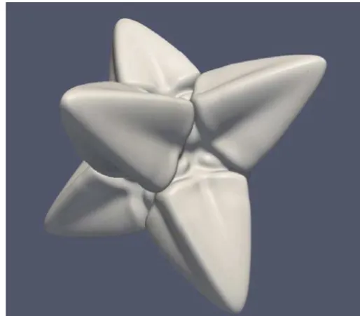
, which sets the temperature oftheliquid’s initialand farboundarycondition below itsfreezing point.As thisparameterbecomes larger theunder-coolingbecomesmoresevere,thesolidificationmorerapidandfractalinappearance:and,also,correspondingly moredifficulttosimulate.

Theotherfield,nothithertodiscussed,isthesolutefield.Forabinaryalloyofinitialconcentration,c_∞,theconcentration of an alloy component atany point is represented by a value ofc

(

x

,

t

)

∈ [

0

,

1

]

. The requirement for equilibriumat the solid-liquidinterface meansthattheconcentrationinthesolidandtheconcentrationintheliquidattheinterfacewillbe unequal. Inasharpinterface modelthisresultsinadiscontinuousjumpinc attheinterface,whileinphasefield models it results ina steep, but continuous, increase inc across the diffuseinterface region, wherethere is some advantage in reformulatingtheproblemtoremovethis.Weshowthisinthenextsection.

2. Governingequations

The governingequationsfordendritic growthofan under-cooledbinary alloy are herepresentedinfull, inboththeir variational formandin the(equivalent) formofPDEs fornumerical implementation.See[8]for afull description ofthe model we employ, derived in turn from[7], which provides analysis of the anti-trapping term, which was extended to isothermaldilutebinaryalloysin[1].TheoriginoftheanisotropyonthelefthandsideofEq.(2a),forexample,isdiscussed in[8]andisvitaltothisformulationineliminatinginterface kineticeffects.Thenon-dimensionalequationsforthephase field,

φ

,thesoluteconcentration,c andthedimensionlesstemperature,

θ

,aregivenviaaspecificationofthefreeenergy.

F

≡

V

1 2A

(n)

2

_∇

_φ

_{· ∇}

_φ

₊

_f

_{(θ, φ)}

_{dV (1)}

andtherelations

τ

(

c

, φ)

A2

(n)

φ

˙

= −

δ

F

δφ

,

(2a)

˙

c

= ∇ ·

K

(φ)

∇

δ

F

δ

c

−

j

,

(2b)

˙

θ

=

Dθ

∇

2

θ

+

1₂

φ.

˙

(2c)

Thesolutediffusionparameterisgivenby

K

=

Dc1₂

(

1

−

φ).

(3)

The parameter Dc is a diffusion constant, thus K

=

0 in the solid (

φ

=

1) and K

=

Dc inthe liquid (

φ

= −

1). Thus, in

general,

φ

∈ [−

1

,

1

]

.Dθ isthetemperaturediffusioncoefficient(assumedconstant).Thenormaltotheinterfaceisgivenby

n

=

∇

φ

|∇

φ

|

,

(4)

whichiswelldefinedaround

φ

=

0,andtheanisotropyfunctionforcubicsymmetry(growthispreferredalongthenormals tothefaces)isgivenforthreedimensionsby[7],

A

(n)

≡

A0

1

+ ˜

n4_x

+

n4_y

+

n4_z

(5)

where n

= [

nx

,

ny

,

nz

]

, A0

=

1

−

3

,

˜

=

4

/(

1

−

3

)

and

≈

0

.

02 governs theamountof anisotropy.Thereasonforthis arrangementofconstantsistocomparewiththetwodimensionalform

A

(n)

≡

A0

1

+ ˜

n4_x

+

n4_y

≡

1

+

cos 4

ψ

(6)

wheretheangle,

ψ

,isgivenby

tan

ψ

=

∂φ

∂

y

/

∂φ

∂

x

.

(7)

Thedimensionlessrelaxationtimefunctionisdefinedby

τ

(

c

, φ)

≡

1

Table 1

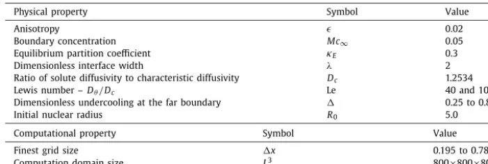
Tableofparametervaluesusedforthesimulationsinthispaper.

Physical property Symbol Value

Anisotropy 0.02

Boundary concentration Mc∞ 0.05

Equilibrium partition coefficient κE 0.3

Dimensionless interface width λ 2

Ratio of solute diffusivity to characteristic diffusivity Dc 1.2534

Lewis number –Dθ/Dc Le 40 and 100

Dimensionless undercooling at the far boundary 0.25 to 0.80

Initial nuclear radius R0 5.0

Computational property Symbol Value

Finest grid size x 0.195 to 0.78

Computation domain size L3 _{800×800×800}

wheretheLewisnumberLe

=

Dθ

/

Dc and

U

≡

1 1

−

kE

2c

/

c_∞

1

+

kE

−

(

1

−

kE

)φ

−

1

.

(9)

HerekE istheequilibriumpartitioncoefficient,c∞ isthefarboundarycondition forc

∈ [

0

,

1

]

.Theanti-trappingcurrentj,

appearinginthesoluteequation,Eq.(2b),isprescribedby

j

= −

1

2

√

2[1

+

(

1

−

kE

)

]U

φn.

˙

(10) Theprofileofc exhibitsaspikeattheinterface, whichcanpresentcomputationaldifficulties.Following[8],thisislargely overcomebyrewritingthesoluteequationusingthevariableU:

1

+

kE

2

−

1

−

kE

2

φ

∂

U

∂

t

= ∇ ·

Dc 1

−

φ

2

∇

U

+

j

+

1

2[1

+

(

1

−

kE

)

U]

∂φ

∂

t

.

(11)

Thephysicaltemperaturefield,T,canberecoveredbytherelationship

θ

=

T

−

TM

−

mc∞

L

/

Cp

,

(12)

whereL andCp arethelatentheatofthephasetransitionandheatcapacityrespectively.Theslopeoftheliquiduslineis

givenbym

=

M L

/

[

Cp

(

1

−

κ

E

)

]

andTM isthemeltingtemperatureofthealloy.

Finallythebulkfreeenergydensityisgivenby

f

(θ, φ,

U

)

≡

φ

2

2

φ

2

2

−

1

+

λ(θ

+

c_∞U

)

φ

−

2

φ

3

3

+

φ

5

5

.

(13)

WesolvethesystemofEqs.(2a),(2c)and(11)plusinitial,typicallysmall,solidseed(seeEq.(40)andSection3.2)andfar boundaryconditions

φ

|

far

= −

1

U

|

far

=

0

(

≡

c

|

far

=

c∞

)

θ

|

far

= −

(14)

where

isthegivenunder-cooling.Theequationfortemperatureisastandarddiffusionequation1 _{withaheatingterm,}

_φ

˙

_, proportionaltothesolidificationrate(orcoolingifmelting).Thedrivingforceforthephaseequationsisgivenby f

(θ,

φ,

U

)

, consistingofadoublewellpotentialhavingstableminimaat

φ

= ±

1 andamaximumat

φ

=

0 andafunctionof

θ

tocreate conditionsformovingthephaseboundary.Forexampleanegativevalueof

θ

createsconditionsfavourableforsolidification. Theparameter,

λ

,isproportionaltotheinterfacewidth,whichinturnischosenasthecharacteristiclengthscale.

2.1. Parametervalues

Forthepurposesofthispaperwechooseaselectionofparameterstouseasdefaultvaluesforthesimulationsbelowin Table 1.Anydeviationfromtheseparametervaluesisexplicitlynotedinthetext.

[image:4.561.95.446.79.197.2]

2.2. Anisotropiccalculations

Notethatthephaseequation,Eq.(2a),ismadeconsiderablymorecomplicatedbythepresenceoftheanisotropyterm,

A

(

n

)

, inthefree energyfunctional.Thevariationalderivative ofa functionalnot involvinggradientsis simplythepartial derivativeofthedensitywithrespecttothatvariable.Thus

δ

δφ

f

(

T

, φ)

dV

=

∂

f

∂φ

=

φ

3

−

φ

+

λ(θ

+

c_∞U

)(

1

−

2

φ

2

+

φ

4

).

(15)

Thevariationalderivativeofthepuregradientpartofthefunctionalisgivenby

δ

G

δφ

≡

δ

δφ

g

(

∇

φ)

dV

= −∇ ·

∂

∂

rg

(r)

r=∇φ

(16)

where,inourmodel,

g

(r)

≡

1₂A

(n)

2

|

r

|

2

,

forr

∈

R

3 (17)

InordertoexpandEq.(16)andthus,Eq.(2a),wefirstintroducethenotation:

φ

,i

≡

∂

i

φ

≡

∂φ

∂

xi etc.,forCartesian

differenti-ation,andsubscriptsfordifferentiationonfunctionspace.Thus

gi

≡

∂

g

∂

ri

,

gi j

≡

∂

∂

ri

∂

g

∂

rj

.

(18)

Thisenablesustowrite

−

δ

G

δφ

=

∂

igi

=

φ

,i jgi j (using the chain rule)

,

whichwrittenoutinfullreads

−

δ

G

δφ

≡ −

δ

δφ

g

(

∇

φ)

dx3

=

∂

2

_φ

∂

xi

_∂

_xj

∂

∂

ri

∂

g

∂

rj

r=∇φ

.

Notethat, gi j,isafunctionofonlyfirstderivativesof

φ

.Toavoidexpandingtheaboveintermsofthecomponents,

φ

,i we

firstintroducethesubstitutionsq

≡ |∇

φ

|

2 andX

≡ [

X1,X2,X3

]

≡ [

φ

2_,1

/

q

,

φ

2_,2

/

q

,

φ

_,2₃

/

q

]

,towritetheanisotropy

A

=

A0

1

+ ˜

3

i=1 X_i2

.

(19)

Foranarbitraryfunctionh

(

r

)

= ˜

h

(

r

,

q

,

X

,

A

)

weusethechainruletowrite

∂

h

∂

ri

=

∂

∂

ri

+

∂

q

∂

ri

∂

∂

q

+

∂

Xj

∂

ri

∂

∂

Xj

+

∂

A

∂

ri

∂

∂

A

˜

h

=

∂

∂

ri

+

2ri

∂

∂

q

+

2ri

q

(δ

i j

−

Xj

)

∂

∂

Xj

+

2ri

q [2A0

˜

Xi

−

2

(

A

−

A0

)

]

∂

∂

A

˜

h

,

(20)

wherewehaveused

∂

q

∂

ri

=

2ri

,

∂

Xj

∂

ri

≡

∂

∂

ri

r2_j

q

=

2ri

δ

i j

q

−

2rir2_j

q2

=

2ri

q

(δ

i j

−

Xj

),

∂

A

∂

ri

=

∂

Xj

∂

ri

∂

A

∂

Xj

=

2ri

q

(δ

i j

−

Xj

)

∂

A

∂

Xj

=

2ri

q

(δ

i j

−

Xj

)

2A0

˜

Xj

=

4ri

using,onthelastsimplification,theidentity A

−

A0

≡

A0

˜

jX2j.Thisallowsustocompute

gi

≡

∂

∂

ri

1 2A

2_q

_|

r=∇φ

=

φ

,iA2

+

4

φ

,i

(

A0Xi

˜

−

A

+

A0

)

A (22)

andfurtherdifferentiationgivestheconciseforms

gii

=

(

24Xi

−

3

)

A2

+

(

−

48Xi2

˜

+

12Xi

˜

−

40Xi

+

4

)

A0A

+

16Xi

(

Xi

˜

+

1

)

2A20

gi j

=

φ

,i

φ

,j

g

24A2

+

(

−

24Xi

˜

−

24Xj

˜

−

40

)

A0A

+

(

16

(

Xj

˜

+

1

))(

Xi

˜

+

1

)

A20

,

i

=

j

.

(23)

Theaboveexpressionsarenotonlymuchmoreconcisethantheexpandedequivalentasafunctionof

φ

,i,butarefunctions

ofXiandAwhichareoforderunityinsizeandthusminimisefloatingpointerrors(theexpandedequivalentcontainstenth

orderpolynomialsof

φ

,i).Wenotealsothat,intheabsenceofanisotropy,

˜

=

0,reduces gi j to

δ

i j sothat

φ

,i jgi j

= ∇

2

φ

.In

thesituationwheregi j isilldefineddueto

|∇

φ

|

→

0 weset.

φ

,i jgi j

|

|∇φ|→0

=

A20

(

1

+ ˜

)

2

∇

2

φ

(24)

or,equivalently A

|

_|∇φ|→0

=

A0(1

+ ˜

)

.Inpracticeweusethisexpressiononlywhen

|∇

φ

|

=

0,tomachineprecisionwithout difficulty.

Usingthenotationtr

(

g

)

≡

δ

i jgi j,therearrangement

φ

,i jgi j

≡

1₃

(φ

,11

+

φ

,22

+

φ

,33

)(

g11

+

g22

+

g33

)

+

(φ

,i j

−

1₃

φ

,kk

δ

i j

)

gi j

≡

1

3

∇

2

φ

tr

(g)

+

(φ

,i j

−

13

φ

,kk

δ

i j

)

gi j

,

(25)

allows the dominant term to be isolated andhas advantage, because the Laplacian can be discretisedto minimise grid induced anisotropy.We willalsoseethat theterm

(φ

,i j

−

1₃

φ

,kk

δ

i j

)

,like gi j,ondiscretisation witha compactstencilata

discretenode,p,onlyhascontributionsfromthenodessurroundingp.Thisaffordssimplificationforthenon-linearsolver laterdiscussed.

2.3. Systemsummary

Writing,Mi j

≡

φ

,i j

−

1₃

φ

,kk

δ

i j wesummarisethenonlinearPDEsystemthatformsourmathematicalmodelas

τ

(

c

, φ)

A

(n)

2

φ

˙

=

₃1

∇

2

φ

tr

(g)

+

Mi jgi j

−

∂

f

∂φ

(26)

where

τ

(

c

,

φ)

isgivenbyEq.(8),

∂

f

∂φ

isgiveninEq.(15),gi j inEq.(23),thesoluteissolvedviaEq.(11),

1

+

kE

2

−

1

−

kE

2

φ

∂

U

∂

t

= ∇ ·

Dc 1

−

φ

2

∇

U

+

j

+

1

2[1

+

(

1

−

kE

)

U]

∂φ

∂

t

,

(27)

andthetemperaturebyEq.(2c),

˙

θ

=

Dθ

∇

2

θ

+

1₂

φ.

˙

(28)

3. Discretisation

The approach taken to discretisation is based upon a cell centred finite difference scheme, in that the nodes of the domain are located atthe centre ofcubic cells, and thus,we usethe term‘node’ and ‘cellcentre’ interchangeably. One consequenceofthisisthat thereare nonodesonthedomain boundary,thusmaking theuseofDirichletboundary con-ditions non-trivial. The scheme makes use of the PARAMESH library to support mesh adaptivity in parallel [11,12]. The meshesobtainedbythisapproachtaketheformofanocttreeofregularblocks,withinwhichthemeshisuniform,andit isthespatial discretisationon anyoneoftheseblocksthatwe discusshere.Subsequentlywe willdiscussadaptivemesh refinementandtheimplicittemporaldiscretisationschemethatisemployed.

3.1. Spatialdiscretisation

Compactfinitedifferencestencils

(

3

×

3

×

3

)

,areusedtodiscretisethefirstandsecondderivatives.Denotingthese27 pointsbyQanddefiningageneric27pointLaplacianstencil,Wabc,aroundapointp

= [

i

,

j

,

k

]

by

∇

2_u

_|

Q

=

1

(

x

)

2 1

a=−1 1

b=−1 1

c=−1

where

xisthephysicaldistancebetweennearestneighbours,wecanrecoverthe7pointLaplacianstencil,builtfromonly thecentrenode,pandthe6nearestneighbours(a2

₊

_b2

₊

_c2

₌

₁₎

∇

2_u

_|

Q

=

−

6ui,j,k

+

ui+1,j,k

+

ui−1,j,k

+

ui,j+1,k

+

ui,j−1,k

+

ui,j,k+1

+

ui,j,k−1

(

x

)

2 (30)

bysettingtheweights

Wabc

=

−

6 a2

+

b2

+

c2

=

0 1 a2

₊

_b2

₊

_c2

₌

₁ 0 otherwise

.

(31)

However,thisstencilismorepronetogridanisotropythanthefollowing27pointLaplacianstencil(see[13]),withweights

Wabc

=

⎧

⎪

⎨

⎪

⎩

−

128

/

30 a2

+

b2

+

c2

=

0 14

/

30 a2

₊

_b2

₊

_c2

₌

₁ 3

/

30 a2

+

b2

+

c2

=

2 1

/

30 a2

+

b2

+

c2

=

3

(32)

Inordertodiscretisethephaseequation,Eq.(26),inspaceitisnecessarytoapproximate

φ

,i jgi j aboutthepointp.Using

theabovenotationweobtain:

(φ

,i jgi j

)

|

Q

=

1₃

∇

2

φ

|

Qtr

(g)

|

(Q−p)

+

Mi j

|

(Q−p)gi j

|

(Q−p)

,

(33)

whereweusethenotation,

|

Q−p,todenotethatthecentralnodeisnotused.ThediscretisationofMi j andgi j aredetailed

inAppendix A. Consequently,Eq.(33)hasthepropertythatonly

∇

2

_φ

_|

Qcontainsacontributionfromthecentral node,

φ

p

andthus

∂

∂φ

p

(φ

,i jgi j

)

|

Q

=

1₃tr

(g)

|

Q−p

∂

∂φ

p

∇

2

_φ

_|

Q

= −

128

90 tr

(g)

|

Q−p

.

(34) ThisisimportantfortheJacobilinearisationdescribedinthenextsection.ThePDEfor

φ

isthusapproximatedbyODEsat eachpoint,p,by

˙

φ

p

=

Fpφ

(φ

Q

,

Up

, θ

p

)

(35)

where

Fφp

≡

1

3

∇

2

φ

|

Qtr

(g)

|

Q−p

+

Mi j

|

Q−pgi j

|

Q−p

−

∂

f

∂φ

(φ

p

,

Up

, θ

p

)

τ

(

cp

, φ

p

)

A2

|

Q−p

.

(36)

Intheabove

τ

(

cp

,

φ

p

)

isgivenbyEq.(8)and

∂

f

∂φ

|

pisgivenbyEq.(15)usingthevaluesfor

φ,

U

,

θ

atpointp.TheLaplacian

∇

2

_φ

_|

QisgivenbyEq.(29)withweightsEq.(32).TheindexedfunctionsMi j aregivenbyEq.(A.1)andthefunctionsgi j are

givenbyEq.(23),where A

,

Xi

,

|∇

φ

|

2 areall functionsof

φ

,i approximatedbysecondorderdifferences, Eq.(A.2).ThePDE

forU,Eq.(11),isapproximatedbytheODEs

˙

Up

=

FpU

(

φ

˙

p

, φ

p

,

UQ

, θ

p

)

(37)

where

F_pU

≡

∇ ·

Dc1−₂φp

∇

U

|

Q

+

j

+

1

2

[

1

+

(

1

−

kE

)

Up

] ˙

φ

p

1+kE

2

−

1−kE

2

φ

p

(38)

whichisexpandedinfull(showninSection3.3)withthesamederivativediscretisationschemeusedforU as

φ

. Finallythe

θ

termisgivenby

˙

θ

p

=

Fpθ

(θ

Q

,

φ

˙

p

)

≡

Dθ

∇

2

θ

|

Q

+

1₂

φ

˙

p

.

(39)

3.2. Boundaryandinitialconditions

WeusezeroNeumannboundaryconditionsforallvariables.Thisiseasilyimplementedbyimposingvaluestothecentre ofghostcellsofallblocksadjacenttotheNeummanboundary,thatareequaltothecentreofthecellvaluesofthosecells next totheboundary(seebelowformorediscussionofghostcells).Inthediscretisation,thissetsallboundaryderivatives equal to zero.In exploitation of the symmetry in the problem this is interpreted as reflective symmetry on the planes

forall variables.If, during a simulation,the normal derivative ofany ofthe dependent variables begins todeviate from zero by more than a prescribed tolerance then we mayallow the domain to expand so as to ensure we retain a zero normalderivative onthe revisedboundary(see belowformoredetails ofthemesh adaptivitythat facilitates this).Fora fixed domain,it is importantthat the dimensionsare sufficient not onlyto representthe growing dendritebut alsothe temperaturefieldthroughoutthesimulation,whichtypicallyextendswellaheadofthephaseinterface(especiallyforlarge valuesoftheLewisnumber).

The physical initial conditions for this problemare not fully understood. One of the sources of theoretical difficulty in modellingthese materials is modellingthe process ofnucleation by which crystallites formvia fluctuations [14]. We adopttheapproachofusingassmallan initialseedaspossibletherebyallowingtheinitialphaseprofile,temperatureand concentrationfieldtoadjustintheveryearlystagesofthesimulation.Thetemperaturefieldcantakelongertoadjusttoa profilewhichisnearthemeltingpointofthealloyinsidethesolidifstartedataconstantfieldvalueand,soweanticipate thiswiththeconditiongivenbelow(seeEq.(41)).

Theinitialconditionforthephasefieldwithseedradiusgivenby Risprescribedby

φ (

t

=

0

,x(p))

= −

tanh

[

α

(

√

x

·

x

−

R

)

]

,

(40)

whereweemploy thefactor

α

=

0

.

6,theprecisevalueofwhichisnot importantasthesolversmoothsthephaseprofile if

α

islargeandconverselysharpentheprofileif

α

istoosmallwithinreason.Itisnotfoundnecessarytonormalisethis profilesothat

φ (

t

=

0

,

x

=

0

)

=

1.TheinitialsoluteconditionisU

=

0 andthetemperatureprofileusedis

θ (

t

=

0

,x(p))

= −

+

1₂

(φ

+

1

).

(41)

The mostsignificant parameterin theinitial conditions,in termsof thesensitivityof thesubsequent calculations, isthe radiusoftheinitialnucleus.Ithasbeenshownthatthetransientbehaviouroftheevolvingdendritecanbeaffectedbythis value wellintothesimulation [15](thoughthefinal geometryandvelocity ofthedendritetipismuch lesssensitive). To thisendwechoosethesmallestvalueof R suchthatthedendritedoesnot melt(meltingcanoccur ifthereisinsufficient solid

φ

=

1 in thenucleusduethe encroachmentof thediffuseinterface near thenucleuscentre). We findthe smallest valuetobeR

≈

5.

3.3. Temporaldiscretisation

DuetothestiffnessofthenonlinearsystemofODEsthatarisesfollowingthespatialdiscretisation weemploythesecond orderBackwardDifferentiationFormula(BDF2[16])timestepping,sothatatapoint,pinthegriddomainatthecentrethe 33 _{points,Q,thephasefieldvariablesystemisapproximatedby}

φ

_pn+1

−

r2

φ

np

+

r3

φ

pn−1

=

r1

tn+1Fφp (42)

Inpractice,weintroduceanothervariable

φ

_p∗

≡

r2

φ

pn

−

r3

φ

pn−1 (43)

andwriteEq.(42)as

φ

n_p+1

−

φ

_p∗

=

r1

tn+1Fpφ

(φ

nQ+1

,

U n+1

p

, θ

pn+1

).

(44)

Therighthandside, Fφp,isdefinedbyEq.(36).

Forconstant timestep,r1

=

2

/

3, r2

=

4

/

3,r3

=

1

/

3.Foragrowing dendriteit isessential tousea smalltimestep at theinitial(imposed)state.Thereafterthetimestepisincreased(seeSection4.2fordetail)tofullyexploittheimplicittime stepping.TheBDF2foradaptivetimesteppingisgivenby

r1

≡

(

r

+

1

)/(

2r

+

1

),

r2

≡

(

r

+

1

)

2

/(

2r

+

1

),

r3

≡

r2

/(

2r

+

1

)

r

≡

tn+1

/

tn (45)

whereristheratioofthecurrenttoprevioustimestep.Theheatequationisdiscretisedsimilarly.With

θ

_p∗

≡

r2θ_pn

−

r3θ_pn−1 wewrite

θ

_pn+1

−

θ

_p∗

=

r1

tn+1Fpθ

(φ

np+1

, φ

p∗

, θ

Qn+1

, θ

p∗

)

(46)

where

F_pθ

(φ

p

, φ

p∗

, θ

Q

, θ

p∗

)

≡

Dθ

∇

2

θ

|

Q

+

1₂

φ

p

−

φ

∗p

r1

tn+1

(47)

3.4. Adaptivemeshandblocktreestructure

The domainis firstdividedinto anumberof meshblockseach ofwhichcontains N

×

N

×

N hexahedralcells, where we typically choose N

=

8. We employ a domain of L3

=

8003, which is large enough forLewis numbers of the order of 100. We divide thisdomain into 43 _{blocks,so that when N}

₌

_{8, each cell isof size 25}3 _{andrefer to thisaslevel 1.} The adaptive mesh strategy then imposes a hierarchicalsub-division ofsome or all these blocks,andtheir descendants, based uponan oct treestructure.Thissubdivisionaims toconcentrate cellswhere gradientsofthe octtreevariables are highest andto ensure neighbourblocks differ by at mostone level.The finestgrid we work withis at level 7, witha corresponding

x

=

25

/

27

₌

₀

_.

_{1953125.Wefindthattheminimumfinestlevelnecessarytoobtainqualitativelyreasonable} resultsislevel 5,corresponding to

x

=

0

.

78125.Asnotedpreviously,throughoutthisworkwe exploitcell-centredfinite differencesinourdiscretisation,inwhicha singleunknownisassociatedwiththecentreofeachhexahedral cellforeach ofthedependentvariables.

Inorderto discussfurtherthetreestructure ofthe blockswedenoteanyblockby itslabel, i andits contents/proper-ties, Bi:

B

(

i

)

= [

l

,

s

,

p

,c,

x

]

(48)

wherel

∈ [

1

,

n

]

isthelevel,s

∈ [

1

,

8

]

isthesiblingnumber(i.e.anindexforwhichchildof ptheblockis),p istheparent index, ci

,

i

∈ [

1

,

8

]

arethe 8 child indices,andx

= [

x

,

y

,

z

]

is the Cartesian positioncoordinates of theblock origin. Any

oneofthesepropertiescanbeaccessedbytheblocknumber,i.Someexamples: p

(

i

)

istheblocknumberoftheparentof block i;x

(

p

(

i

))

isthepositionofthe parent’sorigin;cs(i)

(

p

(

i

))

=

i isan identity. Anaturalpositionschemeforthechild

blocksis

x

(

c1

(

i

))

=

x(i

)

+

1₂

x

[−

1

,

−

1

,

−

1

]

x

(

c2

(

i

))

=

x(i

)

+

1₂

x

[

1

,

−

1

,

−

1

]

x

(

c3

(

i

))

=

x(i

)

+

12

x

[−

1

,

1

,

−

1

]

x

(

c4

(

i

))

=

x(i

)

+

1₂

x

[

1

,

1

,

−

1

]

x

(

c5

(

i

))

=

x(i

)

+

1₂

x

[−

1

,

−

1

,

1

]

x

(

c6

(

i

))

=

x(i

)

+

1₂

x

[

1

,

−

1

,

1

]

x

(

c7

(

i

))

=

x(i

)

+

1₂

x

[−

1

,

1

,

1

]

x

(

c8

(

i

))

=

x(i

)

+

1₂

x

[

1

,

1

,

1

]

,

(49)

where

xisthegridsizeassociatedwithleveli.Acompletespecificationofalltheblocksintheocttreeisthenspecified bythelist:

B

= {

B

(

i

),

i

∈ [

1

,

BN

]}

(50)

where BN isthetotalblock number.Moreover, achildlessblock, i,canbeindicatedby specifying,c

(

i

)

=

0 andsotheoct

treealsocanbespecifiedbyalistingofjusttheleafblocks

B

= {

B

(

i

),

i

∈ [

1

,

BN

] :

c(i

)

=

0

}

.

(51)

There is noadaptive meshingwithin each block, which always contains N

×

N

×

N cells andthe adaptivestrategy is furtherrestrictedbyonlyallowingblocksatlevelnadjacenttoblocksofn

−

1

,

nandn

+

1.Thus,eventhoughablockmay be flaggedforcoarsening,this(latter)restrictionoftenpreventsthishappening. Conversely,blocksflagged forrefinement must,ifnecessary,beaccompaniedbyrefinementonneighbouringblocks.Blocksareflaggedforrefinementif,foranypoint, p,intheblock,thefollowingcriterionissatisfied:

e

≡

max

eφ

|

φ

p

−

φ

p−q

|

,

eU

|

Up

−

Up−q

|

,

eT

|

Tp

−

Tp−q

|

>

η

,

(52)

whereweuse,fortolerance,

η

∼

1 and

|

φ

p

−

φ

p−q

| ≡

(φ

p

−

φ

p−[1,0,0]

)

2

+

(φ

p

−

φ

p−[0,1,0]

)

2

+

(φ

p

−

φ

p−[0,0,1]

)

2

,

(53)

etc.Typicallytheweights,eφ

,

eU andeT arechosentosumtounity.SometimesitisconvenienttoseteU tozerotosuppress

unnecessaryrefinementwithinthesolid.Ife

<

0

.

1

η

,theblockisflaggedforderefinement.

neighbouring blocksviatheguardcellnodes.Whentheneighbouringblockiscoarsertheguardcellofthecoarseblockis foundbyaweightedaverageofthe8 surroundingcoarsenodes(someofwhichareintheparentblock).Usingatri-linear functionofx

,

yandz,givestheweightings,inorderofnearestneighboursfirst

w

=

27 64

,

9 64

,

9 64

,

9 64

,

3 64

,

3 64

,

3 64

,

1 64

.

(54)

Theprocessisknownasprolongation.Forexample,thevalueof

φ

atafinenodeisprolongedby

φ

fine

=

i=coarse cube centres

wi

φ

i

.

(55)

The reverse process, of finding a guardcell value fora coarse block when one or more neighbours isrefined is known asrestrictionandis thesimple averageofthe eightnearest, one levelfiner,cell centres.Both operations, restriction and prolongationusingEq.(54),arealsorequiredformultigridasdetailedinthenextsection.

4. Solvermethod

The discretisation above produces a system of nonlinear algebraic equations for

φ

pn+1

,

Upn+1 and

θ

pn+1 at each time

step,tn+1.In thissection we describe the solutionalgorithm that is used to solve thesesystems,based upon a nonlin-ear multigrid(FullApproximationScheme(FAS) [17]) approach.Initially we describe thenonlinear smootheruponwhich themultigridisbuilt,beforeexploringhowthemultigridsolvercombinesthiswiththehierarchicalmeshadaptivity intro-ducedintheprevioussection.Finally,inSection4.3,weexplainthekeyfeaturesoftheparallelimplementation,including theissuesassociatedwithparalleldynamicload-balancing.

4.1. Nonlinearsmoother

Thenon-linearsystemofalgebraicequationsattheendofSection 3.3canbewrittenusingthegenericvectornotation vn+1

p

≡ [

φ

np+1

,

θ

pn+1

,

Upn+1

]

by

Ap

(v

n_Q+1

)

=

0 (56)

where

Ap

(v

n_Q+1

)

≡

v∗p

−

vpn+1

+

r1

tn+1Fp

(v

n_Q+1

)

(57)

for each node, p, in the grid. Recall, that the appearance of Q indicates coupling between points p and neighbouring nodes,andtheBDF2notation v∗_p incombinationwithr1 are definedinSection 3.3.Using aniterationmethod,withvnp+1

approximatedbyvnp+1,m,wedefinethedefect

dn_p+1,m

= −

Ap

(v

nQ+1,m

).

(58)

ThepointwiseNewtonupdateforthisiterationisgivenby

v_pn+1,m+1

=

v_pn+1,m

−

ω

d

˜

n_p+1,m

,

(59)

whered

˜

pn+1,m isfoundbysolvingthe3

×

3 system

J_pn+1,md

˜

_pn+1,m

≡

dn_p+1,m (60)

withthe3

×

3 Jacobianmatrixdefinedby

Jn_p+1,m

≡

∂d

n+1,m p

∂

vnp+1,m

.

(61)

Inpracticewetypically select,

ω

≈

0

.

9 andfindthatoffdiagonaltermsofJnp+1,m arenotessential toobtainaconvergent

iteration.

ThepreciseformoftheentriesofJnp+1,m maybe deducedfromtheabove.However,we illustratethisindetailforone

ofthediagonaltermsforthesakeofclarity.DenotingthediagonalentriesofJnp+1,m by

[

Jpφ,n+1,m

,

Jθ,pn+1,m

,

JpU,n+1,m

]

,using

Eqs.(44)and(36),andtreatingtermsnotincluding

φ

pasconstantwefind

Jφ,_pn+1,m

≡

∂

d

φ p

(v

nQ+1,m

)

∂φ

p

=

1

+

r1

tn+1 1₃

g11

+

g22

+

g33

τ

(

c

, φ)

A2

128 30

(

x

)

2

p

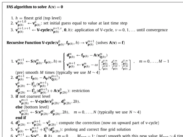
FASalgorithmtosolve A(v)=0

1.h=finestgrid(toplevel) 2.vn_p+_(h1₎,0←vn

p(h):setinitialguessequaltovalueatlasttimestep

3.vn_p+_(h1₎,ν+1←V-cycle(vn_p(+_h1₎,ν,0,h):applicationofV-cycle,ν=0,1,. . .untilconvergence

RecursiveFunctionV-cycle(v0

p(h),fp(h),h)→vmp(+h)1(solvesA(v)=f)

1.vm_p(+_h)1←S(vm

p(h),fp(h),h)≡

⎧ ⎪ ⎨ ⎪ ⎩ dm

p(h)←fp(h)−A(vmQ(h))

vmp(+h)1←v

m

p(h)−ω

_dφ,m p(h)

Jφ,m_p(h), dθ,m_p(h)

J_p(h)θ,m, dU,m_p(h)

JU,m_p(h)

_{, m =0,. . . ,M−1}

(pre)smooth

M

times (typicallyweuse

M

∼4) 2.dmp(+h)1←fp(h)−Ap(vmQ(+h1))

v0 p(2h)←I

h

2h(v m+1 p(h))

d0 p(2h)←I

h

2h(d m+1 p(h))+A(v

0

p(2h)):restriction 3.ifnotcoarsestlevel

vmp(+21h)←V-cycle(v0p(2h),d0p(2h),2h).

else(bottomlevel)

vm_p(+₂1_h)←S(vm

p(2h),d

0

p(2h),2h), m =0,. . . ,N(typicallyweuse

N

∼4)

endif

4.d0 p(2h)←v

m+1 p(2h)−v

0

p(2h):computethecorrection(nowonupwardpartofv-cycle) 5.v0

p(h)←v

m+1 p(h)+I

2h h(d

0

p(2h)):prolongandcorrectfinegridsolution 6.vm_p(+_h)1←S(vm

[image:11.561.112.433.53.293.2]

p(h),0,h), m =0,. . . ,Mpost−1:(post)smoothwiththisnewvalue

M

post∼4 times

Fig. 2.The FAS algorithm.

wherewenotethatthecontributionfromthecentralnodeto

∇

2

φ

is

∂

∇

2

φ

|

Q

∂φ

p

= −

128

30

(

x

)

2

.

(63) Thenewupdatedsolutionfor

φ

attimetn+1_{atiterationmandpointpisgivenby}

φ

_pn+1,m+1

=

φ

n_i+1,m

−

ω

d φ,n+1,m p

Jφ,pn+1,m

.

(64)

Theterm Jθ,pn+1,m

=

1

+

r1tn+1Dθ₃₀128_(x)2 and,thoughtheterm J U,n+1,m

p hasmanycomponents,thelinearityofFpU inUp

leadstostraightforwardupdatesfortheU components,notingthatgradientsinvolvingU

|

Q−paretreatedasconstant.

The above describes a pointwisenon-linear Jacobismoother. The Jacobiapproach lendsitself to parallel implementa-tion since the computation ateach point maybe completed using neighbouringvalues fromthe previous iteration only. Consequently,onlyoneghostcellupdateisrequiredpriortoeachsweepthroughthemesh.Thiskeepsinter-processor com-municationtoaminimum.Usingthestencilsdescribedaboveitispossibletocompletetheupdatesusingjustonelayerof ghostcells.Henceifablocksizeof8

×

8

×

8 (say)isusedinPARAMESHthena10

×

10

×

10 blockisactuallyallocatedto accommodatetheghostlayerofeachblockedge.

Havingderived thepoint-wiseJacobismoother,inthefollowingsubsectionweshow how,thismaybe usedaspartof a non-lineargeometricmultigridsolvercombinedwithlocalmeshadaptivity.Discussionoftheparallel implementationis postponeduntilSection4.3.

4.2. Nonlinearmultigrid

AlthoughtheJacobismootherdescribedabovegivesaconvergentiterationforthesystemEq.(56)(forsufficientlysmall

t andgood initialguess),the convergenceisfar tooslowto beofanypractical use.Fortunately, however,theiteration alsosatisfiesasmoothingpropertywhichmeansthatitdampsout thehighestfrequencycomponentsoftheerror(defect) far more quickly than the rest, see the early chapters of [18] for discussion and analysis of this. This makes it ideally suited for use as part of a nonlinear multigrid scheme. In this work we make use of the Full Approximation Scheme (FAS) ofBrandt[17].We denotethevalueofvariablesatpoint,p,timetn+1_{,iteration,m,andlevel/grid size,hbyv}n+1,m p(h)

and coarser level v_p(n+₂1_h,₎m. The restriction operation, Ih

2h

(

vp(h)

)

,is the assignment to vp(2h) ofthe simple average ofthe 8

surrounding nodes,vp(h).Prolongation, Ih2hvp(2h),is an assignment tovp(h) givenby applyingEq. (54)to give aweighted

average ofthevaluesatthe 8nearest coarsenodes vp(2h).Insolving Eq.(56),FAScomputesa defectfromtherestricted

[image:12.561.133.408.53.253.2]

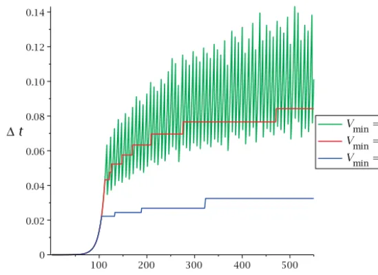
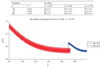
Fig. 3.Anillustration,for

Le

=40,=0.525 oftheevolutionofthetimestep,t,from10−6_{byV-cyclecontrol.(Forinterpretationofthereferencesto}

colourinthisfigurelegend,thereaderisreferredtothewebversionofthisarticle.)

geometricmultigridsolverbydevelopinganimplementationoftheMultiLevelAdaptiveTechnique(MLAT)(see[17]).MLAT allowsustousetheJacobismootheroneachblockwithoutmodification,providedtheprolongationandrestrictionoperators areadaptedtodealwithguardcellsoftheinterfacebetweentoodifferinglevelsofrefinement.Briefly,thesmootherisonly appliedintheregionsofthedomainthatcontain finelevelblocks,butthecoarsegridcorrectiontakesplaceonallpartsof thedomainthatcontain thecoarselevelblocks(thoughthemodified righthandsideassociatedwiththeFASschemeonly contributestothosecoarsegridregionsthathavefinegridsonthem).

Fortheresultspresentedinthefollowingsectionsweareprimarilyinterestedinobtainingsolutionsatlargetimes.Hence we chooseatime-steppingstrategy withthisinmind,basedupon thenumberofnonlinearV-cyclesthat arerequiredto achieveconvergence(foranalternativestrategy,whichusesalocalerrorestimatetocontrol

t,see[19]).Theprincipleis simple:ifthenonlinearmultigridconvergeseasily atagivetimestepthenincrease

t,whereasifitconvergesslowly(or failstoconverge)thendecrease

t (repeatingthetimestepinthecaseoffailure).Convergenceisdeemedtohaveoccurred whentheinfinitynormofthedefect(possiblyweighteddifferentlyforeachdependentvariable),d,satisfiesd

<

dmax,fora user-defined stoppingparameterdmax.IfthisisnotsatisfiedinVfail V-cyclesthen

t ishalvedandthestepisretaken. If convergenceoccursinVminV-cyclesorlessthen

tisincreasedby10% howeverifconvergenceoccursinmorethan Vmax V-cyclesthen

tishalvedforthenextstep.Fig. 3showsatypicalevolutionofthetimestepsizeforthreedifferentchoices ofVmin,baseduponinitial

t

=

10−6,dmax

=

10−10andVmax

=

10.Notethatalthoughtheoscillationin

tisaesthetically undesirableithasnoadverseeffectonthesolutionqualitynor(solongasVmax

<

Vfail)theoverallefficiency.

4.3. Parallelimplementation

Our implementationrequires communication between blocks both on the same level (toapply the smoothingsteps) andbetweenlevels(forprolongationandrestriction).Forparallelprocessing,clearly,communicationbetweencoresneeds tobe kepttoa minimum,butan importantsecondaryconsiderationis thateach corehasasnearaspossible equalload. Forauniformmeshan allocationofeachcoreto anequalvolumeofthecomputationaldomainresultsinanobviousfair division oflabour.Onthe other hand,foranadaptive mesh,such anapproach failssincethe loadingbetweencoreswill differenormously.

Giventhelabel,i,ofeachblockinEq.(48),wepresenttheMortonordering, M

(

i

)

∈ [

1

,

BN

]

,ofanadaptivemesh

M

(

i

)

=

⎧

⎪

⎨

⎪

⎩

1 l

=

1

,

s

=

1 (bottom level)

M

(

p

(

i

))

+

1

,

s

=

1

,

l

>

1 (one plus parent’s label) M

(

s

(

i

−

1

))

+

1

,

s

>

2

,

andl

=

leaf level

M

(

c8

(

i

))

+

1

,

otherwise, i.e.s

=

2

,

(65)

where‘leaflevel’refersanunrefinedlevel(parentwithoutchild)andincludesthefinestlevel.Theblocksmaythenbeput intoaMortonorderedlist:

M(B)

≡ {

Bi

:

j

=

M

(

i

),

j

∈ [

1

,

BN

]}

≡ {

...,

BM(i)

,

BM(j)

, . . .

:

M

(

i

) <

M

(

j

)

}

(66)

LoadbalancingforBN blocksonprocessors pi,i

=

1

,

2

,

. . . ,

cN followsthesameorderwithapproximatelyBN

/

cN blocks

per core. The resulting ordering is well known to exhibit parallel inefficiency for non-uniform meshes. This is because Morton ordering on adaptive meshes leavesthe majority of the top level blocks on a small fractionof cores and since multigrid advances fromthe top tobottom leveland back sequentially,the majorityofthe cores willbe idleat thetop level.Inthreedimensionsthisproblemisacutebecausethereisafactorof8betweenlevels.

Weadoptthefollowingordering,whichmaybetermedMorton-Levelordering. L(B)

≡ {

Bi

:

j

=

L

(

i

),

j

∈ [

1

,

BN

]}

,

≡ {

Lk

(B),

k

∈ [

1

,

n

]}

,

(67)

wherethesubsets,Lk

(

B

)

oneachlevel,karedefined

Lk

(B)

≡ {

...,

BM(i)

,

BM(j)

, . . .

:

M

(

i

) <

M

(

j

),

l

(

i

)

=

l

(

j

)

=

k

}

(68)

Insummary,weimplementadepthfirsttraversaloftheblocksandthen,usingthisnumbering,dividetheworkloadat each levelinturnbetweenall processors.Forauniformmeshthisstrategy resultsina nearoptimum allocationtocores. Foradaptivemeshesthecommunicationonanylevelisalsooptimum,butcommunicationbetweenleveliscompromised.

5. Computationalresults

Thissectionprovidesaselectionofcomputationalresultsthataredesignedtovalidateandassessourproposedsolution algorithm. Since thisis the first attempt to produce three dimensional results for the solidification of a non-isothermal alloy using a realistic interface width we have no external simulations against which to validate our code. Hence the approach taken here has been to firstly validate a two-dimensional restriction of our implementation against our own two-dimensionalsolver,implementedcompletelyindependentlyanddescribedin[19].Thesetestsshowthatweareindeed abletoreproduceresultsfrom[2](e.g.thetipradiusandvelocitiesareinexcellent agreement)eventhoughthetwocode basesarecompletelyindependent,e.g.in[2]fourthorderaccuratestencilswereused.

Furthermore, we have also successfullyvalidated two 3-d simplifications of ourimplementation. In [20] we consider a thermal-onlyrestriction (i.e. a pure metal, so no concentration equation present), where we show quantitative agree-mentwithresultsobtainedusingthe3-d,explicit,thermal-onlyapproachof[21,22].Similarly,in[23]weshowquantitative agreementbetweenanisothermalversion ofoursolver(i.e.notemperatureequationpresent)andanother3-disothermal solidification codedescribedin[21].Tovalidate the3-dnon-isothermalsimulations wenowrelyonhavingmesh conver-genceandmultigridperformance.

Theremainder ofthissectionisdividedintotwosubsections.Thefirstoftheseconsidersthemeshconvergenceofour implementation,showingthatlargetimesolutionsobtainedonasequenceoffinerlevelsofmaximumrefinementdoindeed appearto convergetoparticulardendritegeometries,astestedforaselection ofparametervalues.Thesecond subsection considersthenumericalperformanceofthesolver.Inparticularitisshownthatoptimalperformanceisachieved,whereby thetimerequiredtocompleteatimestepgrowsalmostlinearlywiththetotalnumberofdegreesoffreedom.Thecapability improvementsassociatedwiththedistributedmemoryparallelimplementationarealsodiscussed.

5.1. Meshconvergence

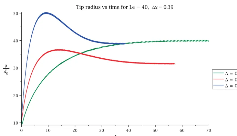
Inordertogainfurtherconfidenceinourcomputationalapproachwehaveundertakenanumberofmeshconvergence tests,inwhichweconsideredcomputationalsimulationsinwhichthemaximumlevelofmeshrefinementissystematically increased.InordertoappreciatetheneedforveryfinegridsatthephaseinterfaceFig. 4illustratesacrosssectionalongthe x-axis of atypicalsolution.Thiscorresponds tothesameparametervaluesasusedtocomputethedendriteillustrated in Fig. 1.Itisclearthatthephasevariable,

φ

,changes

+

1 (bulksolid)to

−

1 (bulkmelt)overaverysmalldistance,similarly thesoluteconcentrationvariesrapidlybothat,andimmediatelyaheadof,theinterface.Thetemperaturevariable,

θ

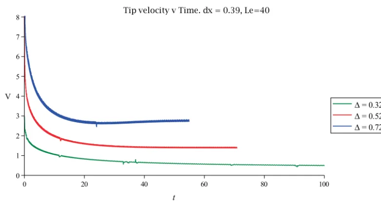
,decays muchmoresmoothlyhowever–thoughalargedomainisrequiredtoensurethattheboundaryeffectdoesnotcontaminate thesolution.Inadditiontotheinterfacewidthafurtherfeatureofsignificant interestisthegeometryofthedendritetip. Fig. 5showsthecomputedevolutionofthetipradiusforthreedifferentundercoolings(0

.

325

,

0

.

525 and0

.

725)atLe

=

40. The parameter, d0

=

5

√

2

/(

8

λ)

is the (non-dimensional) capillarylength asa function of the interface width. Ourvalue for

λ

=

2 gives,d0

=

0

.

44 indicatingthat theinterface widthinour simulationisofthe orderofthe physicalwidth. We use asourcharacteristictime scale,t0

=

0

.

80

(

d

˜

20

λ

3

)/

D

˜

c whered

˜

0 andD

˜

c are thephysicallydimensionedcapillarylength

andsolute diffusivitycoefficientrespectively.Notethat theresultsforFig. 5 werecomputedusingafinemeshspacingof

x

=

0

.

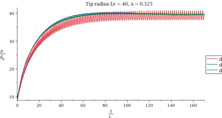
39.Itis an importantquestion toask ifthisissufficiently fineforthe solutionto beinsensitive tofurther mesh refinement.

Fig. 6 shows the computed tip radius as a function of time for three different maximum refinement levels (

x

=

0

.

78

,

0

.

39 and 0

.

195) for case Le

=

40 and

=

0

.

325. The tip radius involves estimating a second derivative of

φ

in theregionwhere

φ

=

0.Thisisundertakenbyestimatingtheradiusonthex-axisat

φ

=

0 usingthephasefield:

r

=

φ

,x

φ

,uu

φ(x,y,z)=0,y=0,z=0

[image:14.561.106.433.72.317.2]

Fig. 4.Thisplotshowsthevariables:phaseφ,soluteconcentration

c

,anddimensionlesstemperatureθ.AtLewisnumberof40andundercoolingof0.525 thetemperaturediffusionzoneextendstoabout300inadomainsizeof8003_{.(Forinterpretationofthereferencestocolourinthisfigurelegend,the}

readerisreferredtothewebversionofthisarticle.)

Fig. 5.Tipradiusat

dx

=0.39 and

Le

=40 forarangeofundercooling.Eventhoughtheradiusat=0.325 takeslongertoreachsteadystate,this simulationisfasterthantheothersduetogreaterstabilityresultinginfewer,largertimesteps.(Forinterpretationofthereferencestocolourinthisfigure legend,thereaderisreferredtothewebversionofthisarticle.)

where

∂

∂

u

=

1

√

2

∂

∂

y

+

∂

∂

z

,

φ

,x

≡

∂φ

∂

x and

φ

,uu

≡

∂

2

φ

∂

u2 (aswillbecomeclearshortly,theu directionismoreconvenient thanthey orzdirections).ExpressionEq.(69)comesfromthedefinition

[image:14.561.70.464.368.594.2]