Energy Efficient Virtual Network Embedding
for Cloud Networks
Leonard Nonde, Taisir E. H. El-Gorashi, and Jaafar M. H. Elmirghani
Abstract—Network virtualization is widely considered to be one
of the main paradigms for the future Internet architecture as it provides a number of advantages including scalability, on demand allocation of network resources, and the promise of efficient use of network resources. In this paper, we propose an energy efficient vir-tual network embedding (EEVNE) approach for cloud computing networks, where power savings are introduced by consolidating re-sources in the network and data centers. We model our approach in an IP over WDM network using mixed integer linear programming (MILP). The performance of the EEVNE approach is compared with two approaches from the literature: the bandwidth cost ap-proach (CostVNE) and the energy aware apap-proach (VNE-EA). The CostVNE approach optimizes the use of available bandwidth, while the VNE-EA approach minimizes the power consumption by re-ducing the number of activated nodes and links without taking into account the granular power consumption of the data centers and the different network devices. The results show that the EEVNE model achieves a maximum power saving of 60% (average 20%) compared to the CostVNE model under an energy inefficient data center power profile. We develop a heuristic, real-time energy op-timized VNE (REOViNE), with power savings approaching those of the EEVNE model. We also compare the different approaches adopting an energy efficient data center power profile. Further-more, we study the impact of delay and node location constraints on the energy efficiency of virtual network embedding. We also show how VNE can impact the design of optimally located data centers for minimal power consumption in cloud networks. Finally, we examine the power savings and spectral efficiency benefits that VNE offers in optical orthogonal division multiplexing networks.
Index Terms—Cloud networks, energy efficient networks, IP
over WDM networks, MILP, network virtualization, optical OFDM, virtual network embedding.
I. INTRODUCTION
T
HE ever growing uptake of cloud computing as a widely accepted computing paradigm calls for novel architectures to support QoS and energy efficiency in networks and data cen-ters [1]. Estimates indicate that in the long term, if current trends continue, the annual energy bill paid by data center operators will exceed the cost of equipment [2]. Given the ecological and economic impact, both academia and industry are focus-ing efforts on developfocus-ing energy efficient paradigms for cloud computing [3].Manuscript received July 23, 2014; revised October 25, 2014 and December 6, 2014; accepted December 6, 2014. Date of publication December 17, 2014; date of current version March 13, 2015. This work was supported by the Engineering and Physical Sciences Research Council (EPSRC), INTERNET (EP/H040536/1), and STAR (EP/K016873/1).
The authors are with the School of Electronic and Electrical Engineering, University of Leeds, Leeds LS2 9JT, U.K.
Color versions of one or more of the figures in this paper are available online at http://ieeexplore.ieee.org.
Digital Object Identifier 10.1109/JLT.2014.2380777
In [4], the authors stated that the success of future cloud net-works where clients are expected to be able to specify the data rate and processing requirements for hosted applications and ser-vices will greatly depend on network virtualization. The form of cloud computing service offering under study here is Infrastruc-ture as a Service (IaaS). IaaS is the delivery of virtualized and dynamically scalable computing power, storage and network-ing on demand to clients on a pay as you go basis. Network virtualization allows multiple heterogeneous virtual network ar-chitectures (comprising virtual nodes and links) to coexist on a shared physical platform, known as the substrate network which is owned and operated by an infrastructure provider (InP) or cloud service provider whose aim is to earn a profit from leasing network resources to its customers (Service Providers (SPs)) [5]. It provides scalability, customised and on demand allocation of resources and the promise of efficient use of net-work resources [6]. Netnet-work virtualization is therefore a strong proponent for the realization of an efficient IaaS framework in cloud networks. InPs should have a resource allocation frame-work that reserves and allocates physical resources to elements such as virtual nodes and virtual links. Resource allocation is done using a class of algorithms commonly known as “virtual network embedding (VNE)” algorithms. The dynamic mapping of virtual resources onto the physical hardware maximizes the benefits gained from existing hardware [7]. The VNE problem can be either Offline or Online. In offline problems [8] all the virtual network requests (VNRs) are known and scheduled in advance while for the online problem, VNRs arrive dynami-cally and can stay in the network for an arbitrary duration [9], [10]. Both online and offline problems are known to be NP-hard. With constraints on virtual nodes and links, the offline VNE problem can be reduced to the NP-hard multiway separa-tor problem [11], as a result, most of the work done in this area has focused on the design of heuristic algorithms and the use of networks with minimal complexity when solving mixed integer linear programming (MILP) models.
Network virtualization has been proposed as an enabler of en-ergy savings by means of resource consolidation [8], [12]–[15]. In all these proposals, the VNE models and/or algorithms do not address the link embedding problem as a multi-layer problem spanning from the virtualization layer through the IP layer and all the way to the optical layer. Except for the authors in [14], the others do not consider the power consumption of network ports/links as being related to the actual traffic passing through them. On the contrary, we take a very generic, detailed and ac-curate approach towards energy efficient VNE (EEVNE) where we allow the model to decide the optimum approach to minimize the total network and data centers server power consumption.
We consider the granular power consumption of various network elements that form the network engine in backbone networks as well as the power consumption in data centers. We develop a MILP model and a real-time heuristic to represent the EEVNE approach for clouds in IP over WDM networks with data cen-ters. We study the energy efficiency considering two different power consumption profiles for servers in data centers;
An energy inefficient power profile and an energy efficient power profile. Our work also investigates the impact of location and delay constraints in a practical enterprise solution of VNE in clouds. Furthermore we show how VNE can impact the design problem of optimally locating data centers for minimal power consumption in cloud networks.
The remainder of the paper is organized as follows: We ex-amine related work in Section II. The EEVNE MILP model and heuristic are introduced in Section III and Section IV, respec-tively. The EEVNE approach is evaluated and compared to the CostVNE and the VNE-EA approaches in Section V. In Section VI we re-evaluate the energy efficiency of the EEVNE approach considering an energy efficient data center power profile and in Section VII, we investigate the impact of location and delay constraints on the energy efficiency of VNE. In Section VIII we solve the VNE design problem of optimally locating data centers for minimal power consumption in cloud networks. We introduce VNE in O-OFDM cloud networks in Section IX and we finally conclude the paper in Section X.
II. RELATEDWORK
The VNE problem has been extensively investigated in the literature from different perspectives such as load balancing in the substrate network [14], [16], [17] and efficient use of re-sources [9]. We have investigated the VNE problem for profit maximization by InPs in cloud networks [18]. We developed a MILP model and showed that higher acceptance rates do not necessarily lead to higher profit due to the high cost associated with accepting some of the VNRs. We also showed that despite the profit maximized model showing slightly higher power con-sumption than the power minimized model, it still performed better because the profit achieved by the profit maximized model is higher than the increase in power consumption when the latter is expressed in monitory terms. In [19] the authors developed a MILP model which attempts to minimize the bandwidth cost of embedding a VNR. In [12] the virtual network embedding energy aware (VNE-EA) model minimized the energy consump-tion by imposing the noconsump-tion that the power consumpconsump-tion is min-imized by switching off substrate links and nodes. The authors also assume that the power saved in switching off a substrate link is the same as the power saved by switching off a substrate node. In [13] the authors assumed that the power consumption in the network is insensitive to the number of ports used. They also seek to minimize the number of active working nodes and links. Botero and Hesselbach [14] have proposed a model for energy efficiency using load balancing and have also developed a dynamic heuristic that reconfigures the embedding for energy efficiency once it is performed. They have implemented and evaluated their MILP models and heuristic algorithms using the
ALEVIN Framework [20]. The ALEVIN Framework is a good tool for developing, comparing and analyzing VNE algorithms. We are however unable to compare our model and heuristic to the implemented algorithms on the platform for the following reasons:
1. Our input parameters are not compatible to the existing models and algorithms on the platform. Extensive exten-sions to the algorithms and models would be needed for them to include the optical layer. Our parameters include among others; the distance in km between links for us to determine the number of EDFA’s or Regenerators needed on a link, the wavelength rate, the number of wavelengths in a fiber, the power consumption of EDFAs, transpon-ders, regenerators, router ports, optical cross connects, multiplexers, de-multiplexers, etc.
2. The assumptions made in the calculation of power in our model and the models on the platform are different. We define the power consumption to its fine granularity to in-clude power consumed due to traffic on each element that forms the network engine. One of our main contributions in this work is the inclusion of the optical layer in link embedding which is currently not supported by any of the algorithms on the ALEVIN platform.
Wang et al. [8] developed a generalized power consumption model of embedding a VNR and formulated it as a MILP model; however, they also assumed that the power consumption of the network ports is independent of traffic. In [15] the authors pro-pose a trade-off between maximizing the number of VNRs that can be accommodated by the InP and minimizing the energy cost of the whole system. They propose embedding requests in regions with the lowest electricity cost.
III. ENERGYEFFICIENTVIRTUALNETWORKEMBEDDING
A. Virtual Networks in IP Over WDM Networks
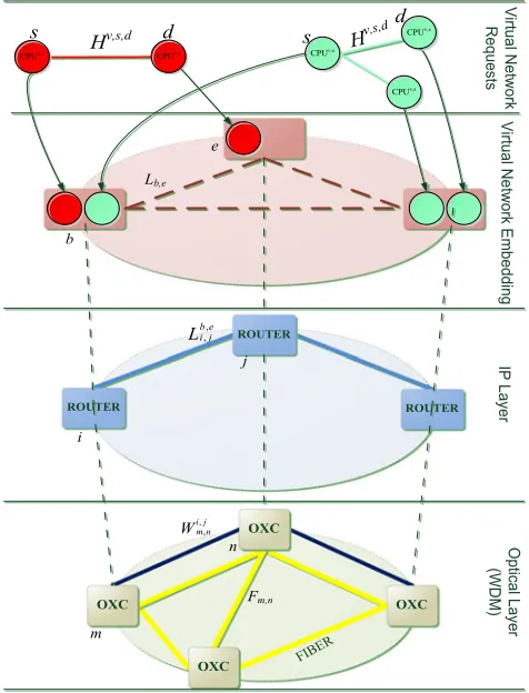
Fig. 1. Virtual network embedding in IP over WDM architecture.
to the IP and optical equipment. The node demands of the VNRs are embedded in the data centers. When a virtual node is embedded in the substrate network, its CPU demands instantiate virtual servers in the data center and its bandwidth demands in-stantiate a virtual router in the core router such that the requester of the service is granted control of both the virtual servers and virtual router and has the ability to configure any protocols and run any applications.
B. MILP Model for EEVNE
In this section we develop a MILP model to minimize the total power consumption of the IP over WDM architecture with data centers shown in Fig. 1 by optimizing the embedding of VNRs.
The substrate network is modeled as a weighted undirected graphG= (N, L)whereN is the set of substrate nodes andL is the set of substrate links. Each node or link in the substrate network is associated with its own resource attributes. The VNR v is represented by the graphGv = (Rv, Lv)where Rv is the
set of virtual nodes andLvis the set of virtual links. In Fig. 2, we
illustrate how demands in a VNR are mapped onto the substrate network across multiple layers. We clearly show where some of the variables and parameters used are located across the layers. Before introducing the model, we define the sets, parameters and variables used;
Sets:
V Set of VNRs;
R Set of nodes in a VNR;
N Set of nodes in the substrate network;
Nm Set of neighbor nodes of nodemin the optical layer;
Parameters:
s and d Index the source and destination nodes in the topol-ogy of a VNR;
b and e Index source and destination substrate nodes of an end to end traffic demand aggregated from all VNRs;
i and j Index the nodes in the virtual lightpath topology (IP layer) of the substrate network;
Fig. 2. Illustration of VNE across multiple layers in IP/WDM.
m and n Index the nodes in the physical topology (optical layer) of the substrate network;
CPUb Available CPU resources at substrate node (data
center)b;
Nb Number of servers at substrate nodeb;
NCPUv ,s Number of the servers required by VNRvin node s;
CPUv ,sb CPUv ,sb = NC PUv , s
Nb , is the percentage CPU
[image:3.594.311.549.281.593.2]Hv ,s,d Bandwidth requested by VNR v on virtual link
(s,d);
B Wavelength rate;
W Number of wavelengths per fiber; Dm ,n Length of the physical link (m, n);
DOb DOb = 1if the data center at nodebhas been
ac-tivated by previous embeddings;
Fm ,n Number of fibers in physical link(m, n);
EAm ,n Number of EDFAs in physical link(m, n).
Typi-callyEAm ,n =
Dm , n S
−1+ 2, where S is the distance between two neighboring EDFAs; P R Power consumption of a router Port; P T Power consumption of a transponder; P E Power consumption of an EDFA;
P Om Power consumption of an optical switch at nodem; PMD Power consumption of a multi/demultiplexer; DMm Number of multi/demultiplexers at nodem;
Pidle Idle server power consumption of a data center;
μ Data center server power consumption per 1% CPU load.
Variables:
δv ,sb δbv ,s= 1, if nodesof VNRvis embedded in a substrate nodeb, otherwiseδbv ,s = 0;
Ψv Ψv = 1, if all the nodes of a VNRvare fully embedded in the substrate network, otherwiseΨv = 0;
ρv ,s,db,e ρv ,s,db,e = 1, if the embedding of virtual nodessanddof virtual requestvin substrate nodesbande, respectively is successful and a link b, eis established if a virtual links, dof VNRvexists.
ωb,ev ,s,d ωv ,s,db,e is the XOR ofδv ,sb andδv ,d e , i.e.ω
v ,s,d b,e =δ
v ,s b ⊕
δv ,d e ;
Lb,e Traffic demand between the substrate node pair (b, e)
aggregated from all embedded VNRs;
Φv Φv = 1, if all the links of VNRvare fully embedded in the substrate network, otherwiseΦv = 0;
Lb,ei,j Amount of traffic demand between node pair(b, e) pass-ing through the lightpath(i, j)in the substrate network; Ci,j Number of wavelengths in lightpath(i, j)in the
sub-strate network;
Qb Number of aggregation router ports at nodeb;
Wi,j
m ,n The number of wavelengths of lightpath (i, j)passing
through a physical link(m, n);
Wm ,n Number of wavelengths in physical link(m, n);
λm ,n λm ,n = 1, if the physical link(m, n)is activated
other-wiseλm ,n = 0;
Kb Kb = 1if the data center in nodebis activated,
other-wiseKb = 0.
The total power consumption is composed of the power con-sumption in data centers and the power concon-sumption in the network.
[image:4.594.325.524.63.186.2]As discussed in [22] the CPU utilization is the main contrib-utor to the power consumption variations in a server. Therefore the CPU utilization of servers in a data center is also the main contributor to the variation in the power consumption of a data center. We only consider the servers power consumption when calculating the power consumption of data centers as the largest
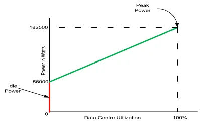
Fig. 3. Data center servers power profile with 500 Dell R720 servers.
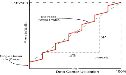
proportion of data center power is drawn by Servers. Accord-ing to [23], 59% of the power delivered in the data center goes to IT equipment. It also states that decreasing the power draw of servers clearly has the largest impact on the power cost in data centers. While we appreciate the efforts done by other researchers and institutions like Google and Microsoft in im-proving the energy consumption due to cooling and the use of efficient power supplies, our efforts in the paper are restricted to the power consumed in servers and high capacity network equipment in data centers. It is worth noting here that large data centers have now achieved power usage effectiveness (PUE) approaching 1, for example [24] and [25] report PUE values of 1.12 and 1.125 respectively, where it is clear that the data cen-ter servers (and communication equipment) power consumption now dominates in large data centers compared to cooling, light-ing and power supply units losses. The power consumption due to the local area network (LAN) inside the data center also con-tributes to the power consumption in the data center. However, as we will show later, the LAN power consumption is very low compared to the power consumption due to servers. We there-fore consider the energy inefficient data center power profile shown in Fig. 3 which considers only the power consumption due to servers. The power profile in Fig. 3 is constructed from a data center containing 500 Dell Power Edge R720 Servers [26] each with idle power rated at 112W and 365W at full load. The power consumption in a data center due to the embedding of nodesof VNRvis given as:
P Dbv ,s
=
Pidle+μ·CPUv ,sb , if the data centre atbis ON
0, otherwise.
The power consumption of data centers due to servers is given as:
P D= b∈N
v∈V
s∈R
CPUv ,sb ·δbv ,s·μ+Kb·Pidle.
Power consumption of router ports:
m∈N
P R·
Qm +
n∈Nm
Wm ,n
.
Power consumption of transponders:
m∈N
n∈Nm
P T ·Wm ,n.
Power consumption of EDFAs:
m∈N
n∈Nm
P E·EAm ,n ·Fm ,n ·λm ,n.
Power consumption of optical switches:
m∈N
P Om.
Power Consumption of multi/demultiplexers:
m∈N
PMD·DMm
The model is defined as follows: Objective:
Minimize the overall power consumption in the network and data centers given as:
m∈N
P R·
Qm+
n∈Nm
Wm ,n
+
m∈N
n∈Nm
P T ·Wm ,n
+
m∈N
n∈Nm
P E·EAm ,n ·Fm ,n·λm ,n +
m∈N
P Om
+
m∈N
PMD·DMm
+
b∈N:D Ob= 0
v∈V
s∈R
CPUv ,sb ·δv ,sb ·μ+KbPidle. (1) Subject to:
VNRs constraints:
v∈V
s∈R
CPUv ,sb ·δv ,sb ≤CPUb b∈N. (2)
Constraint (2) ensures that the CPU demands allocated to a substrate node do not exceed the capacity of its data center
b∈N
δv ,sb = 1 ∀v∈V, ∀s∈R. (3) Constraint (3) ensures that each node in a VNR is embedded only once in the substrate network
δv ,sb +δev ,d =ωe,bv ,d,s+ 2·ρv ,s,db,e
∀v∈V, ∀b, e∈N :b= e, ∀s, d∈R:s=d. (4) Constraint (4) ensures that virtual nodes connected in the VNR are also connected in the substrate network. We achieve this by introducing a binary variableωv ,d,se,b which is only equal to 1 ifδbv ,sandδev ,dare exclusively equal to 1 otherwise it is zero
ρv ,s,db,e =ρv ,d,sb,e
∀v∈V, ∀b, e∈N :b= e ∀s, d∈R:s=d. (5) Constraint (12) ensures that the bidirectional traffic flows are maintained after embedding the virtual links
v∈V
s∈N
d∈N:s=d
Hv ,s,d·ρv ,s,db,e =Lb,e ∀b, e∈N :b=e.
(6) Constraint (6) generates the traffic demand matrix resulting from embedding the VNRs in the substrate network and ensures that no connected nodes from the same VNR are embedded in the same substrate node
bεN
s∈R
CPUv ,sb ·δv ,sb = Ψv bεN
s∈R
CPUv ,sb ∀v∈V. (7) Constraint (7) ensures that nodes of a VNR are completely embedded meeting their CPU demands
b∈N
e∈N:b=e
s∈R
d∈R:s=d
Hv ,s,d·ρv ,s,db,e
= Φv s∈R
d∈R:s=d
Hv ,s,d ∀v∈V. (8)
Constraint (8) ensures the bandwidth demands of a request are completely embedded
Φv = Ψv ∀v∈V. (9)
Constraint (9) ensures that both nodes and links of a VNR are embedded. Constraints (7)–(9) collectively ensure that a request is not partially embedded.
Flow conservation in the IP Layer
j∈N:i=j
Lb,ei,j −
j∈N:i=j
Lb,ej,i =
⎧ ⎪ ⎨ ⎪ ⎩
Lb,e, ifi=b
−Lb,e, ifi=e 0, otherwise.
∀b, e, i∈N :b=e (10)
Constraint (10) represents the flow conservation constraint for the traffic flows in the IP Layer.
Lightpath capacity constraint
b∈N
e∈N:b=e
Lb,ei,j ≤Ci,j·B ∀i, j∈N :i=j. (11)
Constraint (11) ensures that the sum of all traffic flows through a virtual link does not exceed its capacity.
Flow conservation in the optical layer
n∈Nm
Wm ,ni,j −
n∈Nm
Wn ,mi,j =
⎧ ⎪ ⎨ ⎪ ⎩
Ci,j, if m=i
−Ci,j, if m=j 0, otherwise.
∀i, j, m∈N :i=j (12)
Constraint (12) ensures the conservation of flows in the optical layer.
Physical link capacity constraints
i∈N
j∈N:i=j
(a)
[image:6.594.302.548.60.600.2](b)
Fig. 4. Grouping of nodes of a VNR 1 (a) A VNR requiring a minimum of two substrate nodes (b) A VNR requiring a minimum of three substrate nodes.
i∈N
j∈N:i=j
Wm ,ni,j =Wm ,n. ∀m∈N, n∈Nm (14)
Constraints (13) and (14) represent the physical link capacity constraints. Constraint (13) ensures that the number of wave-lengths in a physical link does not exceed the capacity of fibers in the physical links. Constraint (14) gives the total number of wavelength channels used in a physical link.
Aggregation ports constraint
Qb =
e∈N:e=b
Lb,e/B ∀b∈N. (15)
Constraint (15) gives the number of aggregation router ports at each node in the substrate network.
IV. THEREAL-TIMEENERGYOPTIMIZEDVIRTUALNETWORK EMBEDDING(REOVINE) HEURISTIC
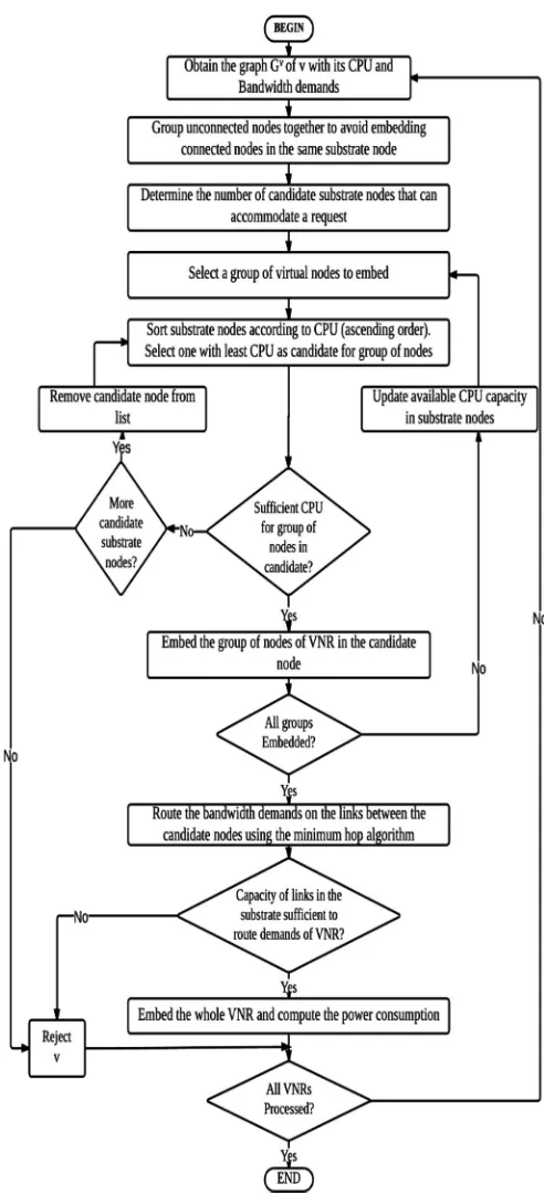
The (real-time energy optimized virtual network embedding) (REOViNE) heuristic provides real-time implementation of the EEVNE approach. The flow chart of the heuristic is shown in Fig. 5. The heuristic obtains the graphGv = (Rv, Lv)of VNR v. The nodes of v are grouped such that those that are not connected to each other in the VNR topology graph Gv are put into one group. Separate groups are created for all the other nodes that are connected to each other to avoid embedding nodes that are connected in the VNR into the same substrate node. The heuristic determines the number of candidate substrate nodes required to embed a full VNR based on the number of node groups created. Fig. 4 shows examples of nodes grouping of a VNR with four nodes and three links. In Fig. 4(a), Nodes 1 and
Fig. 5. REOViNE heuristic flow chart.
[image:6.594.45.288.67.335.2]Similarly node 2 has to be in a group of its own. The grouping in Fig. 4(b) results in 3 substrate nodes, whereas Fig. 4(a) grouping needs only 2 substrate nodes to embed the VNR. The grouping is done to achieve maximum compaction, i.e. minimum number of substrate nodes. Therefore the grouping in Fig. 4(a) will be selected as the optimal grouping. From the example above we can summarize the rules of grouping as follows:
i. Nodes that are not connected in the virtual request can be grouped in one group and embedded in the same substrate node.
ii. Nodes that are connected to each other must belong to different groups.
iii. The grouping process is only finished when all nodes in the virtual request have found a group.
iv. There may be more than one grouping option. The group-ing option that leads to the minimum number of substrate nodes is selected.
The substrate nodes are sorted according to the available CPU capacity in ascending order. Because of the energy inefficient power profile of the data centers (large idle power), the heuristic tries to consolidate the embeddings in data centers by filling the ones with least residual capacity before switching on oth-ers. The substrate node with the least available CPU capacity is selected as the candidate to embed the first group of nodes. The order in which the groups are selected is not important because it does not affect the success or failure of the embedding of nodes. However, we select the grouping option that requires the minimum number of substrate nodes. If the candidate substrate node has sufficient capacity, the virtual nodes will be embedded in that substrate node; otherwise the heuristic will try to embed the virtual nodes in another substrate node. If, however, we have exhausted all the candidate substrate nodes, the request will be rejected and the heuristic will proceed to embed another request. After embedding all the nodes of the VNR, the heuristic tries to route the bandwidth demands on the links between the candidate substrate nodes using the minimum hop algorithm to minimize the network power consumption. The request will be blocked if any of the links does not have sufficient capacity to accommo-date the traffic. If the traffic is successfully routed, the request is accepted. The heuristic calculates the power consumption of the accepted request and continues to embed other VNRs.
V. PERFORMANCEEVALUATION
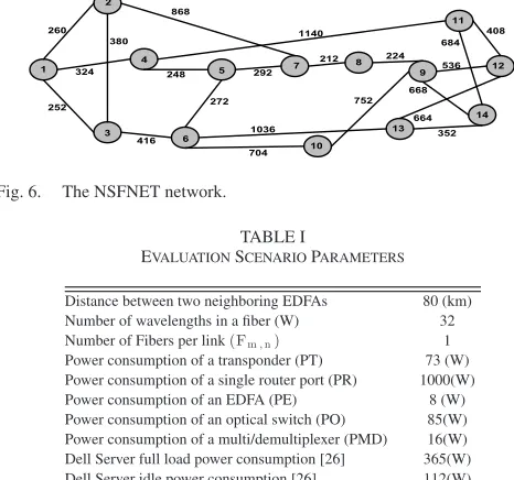
To evaluate the performance of the proposed model and heuristic, the NSFNET network is used as the substrate net-work. NSFNET comprises 14 nodes and 21 links as shown in Fig. 6. We consider a scenario in which each node in NSFNET hosts a small data center of 500 servers to offer cloud services. Table I shows the parameters used. The power consumption of the network devices we have used are consistent with our previous work in [27] which are derived from [28]–[32]. The IP router ports are the most energy consuming devices in the network.
[image:7.594.307.540.71.289.2]We have adopted the Dell Power Edge R720 [26] server power specifications. We adapted the CostVNE model [20] and the VNE-EA model [12] for the IP over WDM network architecture
Fig. 6. The NSFNET network.
TABLE I
EVALUATIONSCENARIOPARAMETERS
Distance between two neighboring EDFAs 80 (km) Number of wavelengths in a fiber (W) 32 Number of Fibers per link(Fm,n) 1
Power consumption of a transponder (PT) 73 (W) Power consumption of a single router port (PR) 1000(W) Power consumption of an EDFA (PE) 8 (W) Power consumption of an optical switch (PO) 85(W) Power consumption of a multi/demultiplexer (PMD) 16(W) Dell Server full load power consumption [26] 365(W) Dell Server idle power consumption [26] 112(W) Data Center idle power consumption (500 servers) 56 000(W)
and compared their performance to our EEVNE model and the REOViNE heuristic in terms of power consumption and number of accepted requests. The objective functions of the two models are as follows:
CostVNE Model Objective
The CostVNE model minimizes the substrate resources allo-cated to a VNR. Since the amount of CPU resources alloallo-cated to a request cannot be reduced through consolidation, the model only optimizes the use of bandwidth on the links by consolidat-ing wavelengths. The objective of the CostVNE model is given as:
minimize
m∈N
n∈Nm
Wm ,n
VNE-EA Objective
The VNE-EA model [12] minimizes the energy consumption by minimizing the number of substrate links and nodes that are activated when embedding VNRs. The objective function of this model is given as:
minimize
m∈N:N Om= 0 σm +
m∈N
n∈Nm:L Om , n= 0
βm ,n
whereσm andβm ,nare binary variables that indicate the active
nodes and links in the substrate network, respectively. Note that N Om and LOm ,n are binary parameters indicating the
already activated substrate nodes and links, respectively before the embedding of requests.
A. Embedding of VNRs of Uniform Load Distribution
2 and 6. The CPU demand of nodes in the VNR is uniformly distributed between 2% and 10% of the total CPU resources of a data center. The bandwidth on links of the VNR is also uniformly distributed between 10 and 130 Gb/s. We have considered em-bedding 50 VNRs onto the 14 node NSFNET substrate network. The AMPL software with the CPLEX 12.5 solver is used as the platform for solving the MILP models and REOViNE was implemented in Matlab. All the Models and REOViNE were executed on a PC with an Intel Core i5–2500 CPU, running at 3.30 GHz, with 8 GB RAM.
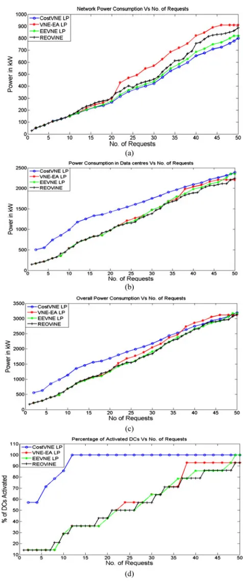
The results in Fig. 7 show the network power consumption, the data centers power consumption and the overall power con-sumption versus the number of VNRs. The requests arrive two at an instance and the existing requests are not reconfigured when embedding arriving requests.
The CostVNE model has resulted in the minimum network power consumption as it optimizes the use of bandwidth of the substrate network by consolidating wavelengths regardless of the number of data centers activated (see Fig. 7(a)). Compared to the EEVNE model, the CostVNE model has saved a maximum of 5% (average 3%) of the network power consumption. The EEVNE model, where the energy consumption is minimized by jointly optimizing the use of network resources and consolidat-ing resources in data centers, has resulted in better power savconsolidat-ings compared to the VNE-EA model where the power consumption is minimized by switching off substrate links and nodes. This is because the network power consumption is mainly a function of the number of wavelengths rather than the number of active links as the number of wavelengths used determines the power consumption of router ports and transponders, the most power consuming devices in the network (see Table I). The REOViNE heuristic approaches the EEVNE model in terms of the network power consumption.
Fig. 7(b) shows the power consumption of data centers un-der the different models and heuristic. As mentioned above, the CostVNE model does not take into account the number of acti-vated data centers, therefore it performs very poorly as far as the power consumption in data centers is concerned. However, as the network gets fully loaded and all the data centers are activated, the EEVNE model loses its merit over the CostVNE model. For a limited number of requests, the VNE-EA model performs just as good as the EEVNE model. However as the number of requests increases, the VNE-EA model tends to route the virtual links through multiple hops to minimize the number of activated links and data centers and therefore consumes more power. The REOViNE heuristic also approaches the EEVNE performance in terms of the data centers power consumption.
[image:8.594.307.545.60.629.2]Since the power consumption of the data centers is the main contributor to the total power consumption (given the power consumption of servers and network devices (see Table I)), the total power consumption, shown in Fig. 7(c), follows similar trends to that of the data centers. In the best case over a span of 50 VNRs, the EEVNE model saves 60% of the overall power consumption compared to the CostVNE model with an average saving of 21%. Compared to the VNE-EA model, the EEVNE model achieves maximum combined data center and network power savings of 9% (3% on average).
Fig. 7. (a) Network power consumption of the different approaches, (b) DCs power consumption of the different approaches, (c) Overall power consumption of the different approaches, (d) Data center activation of the different approaches.
Fig. 8. Number of accepted requests.
Fig. 9. Cloud data center architecture.
The revenue of a virtual network service provider can be greatly affected by its inability to accept new requests. Fig. 8 shows the number of accepted requests for the different models and the REOViNE heuristic. In an evaluation scenario with suf-ficient CPU resources to embed all virtual nodes, the CostVNE model has accepted all the 50 requests as it efficiently utilizes the network bandwidth. The improved energy efficiency achieved by the EEVNE model has a limited effect on its ability to ac-cept VNRs. The EEVNE model has however only rejected one request. The REOViNE heuristic rejected three requests. The VNE-EA model is the worst performer in terms of accepted requests with four rejected requests. This arises as the VNE-EA model tries to fully use activated links before turning on more links therefore depleting the capacity on links to certain des-tinations. It therefore fails to map VNRs despite the substrate network having sufficient CPU resources.
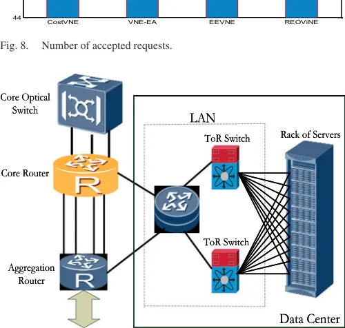
As mentioned earlier in Section III-B, the power consump-tion of the LAN inside the data centre contributes to the overall power consumption of the data centre. Fig. 9 below shows a typical architecture of the cloud data centre and how it is con-nected to the core network. Typically, data centres are built very close to the core network nodes to benefit from the large
band-width capacities available from such nodes. If the data centre is serving users located at this node, the traffic flows from the servers onto the top of the rack (ToR) switches, then to the LAN router located inside the data centre and eventually to the ag-gregation router. The traffic serving users located at other core nodes flows to the core router and is then switched by the high capacity optical switch to the desired destination. The server power consumption is proportional to the amount of process-ing required by the embedded VNRs while the network power consumption inside the data center is proportional to the traf-fic generated by the requests. For example a low bandwidth and processing intensive VNR such as gaming will present low traffic and thus low power consumption in the network inside a data center but very high server power consumption. On the other hand, the network inside the data center will consume high power when embedding VNRs demanding high bandwidth and low processing like video streaming.
We have extended the EEVNE model to take into account the power consumption due to the LAN inside the data centre. We define the following additional variables and parameters in the model:
T oR P C LAN ToR switch power consumption; T oR C LAN ToR switch switching capacity;
T oR P P B LAN ToR switch energy per bit,T oR P P B=
T oR P C/T oR C;
R P C LAN Router power consumption; R C LAN Router routing capacity;
R P P B LAN Router energy per bit, R P P B=
R P C/R C;
The power consumption of both the LAN ToR switches and routers inside the data center (LANPC_DC) is proportional to the traffic inside the data center [33] and can be given as
LANPC DC =
b∈N
e∈N:e=b
Lb,e·(T oR P P B+R P P B).
Therefore, the data center power consumption which includes both servers and the LAN (PDC) becomes:
PDC =
b∈N
v∈V
s∈R
CPUv ,sb ·δbv ,s·μ+Kb·Pidle
+
b∈N
e∈N:e=b
Lb,e·(T oR P P B+R P P B).
The Cisco Catalyst 4900M switch [34] with a capacity of 320 Gb/s and power rating of 1 kW was considered as the ToR switch. The Cisco 7613 Router [35] rated at 720 Gb/s and 4 kW was considered as the data center LAN router.
Fig. 10 shows the power consumption in data centers due to servers and due to the LAN. It can be seen that the power consumption due to servers dominates the power consumption due to the LAN. The LAN power consumption only accounts for 4% of the total power inside the data center. The inclusion of the LAN power consumption has also had no effect on the way the nodes and links are embedded across the network.
Fig. 10. Power consumption in dc due to servers and LAN.
Fig. 11. Network power consumption in the Core and the dc LAN.
TABLE II
PERFORMANCE OFREOVINEANDEEVNEINDIFFERENTNETWORKS
Substrate Network Method Request Acceptance Running Time
NSFNET EEVNE 49/50, 98% 85 000 s
Random Topology 10 Nodes 23 Links EEVNE 34/50, 68% 64 800 s Random Topology 8 Nodes 14 Links EEVNE 28/50, 56% 39 600 s
NSFNET REOViNE 47/50, 94% 7 s
USNET REOViNE 49/50, 98% 40 s
ITALIA REOViNE 49/50, 98% 28 s
the power consumption in the core when handling the same amount of traffic because the core network comprises more equipment and routes traffic over much longer distances.
In order to investigate the scalability of our energy efficient VNE approach, we evaluated our model (EEVNE) in small randomly generated topologies and our heuristic (REOViNE) in large network topologies since testing complex MILP models like ours on large networks often leads to huge complexities and unaffordable execution times. The topology matrices and associated distances of the randomly generated networks were produced in MATLAB with link distances randomly distributed between 100 and 1500 km. For the large networks we considered the 24-node 43-link USNET [21] substrate network and the 21-node 36-link Italian network [36]. Table II shows the acceptance ratio and the running times for the different topologies under the same load.
Fig. 12. REOViNE and EEVNE model overall power consumption in different networks.
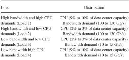
TABLE III LOADDISTRIBUTIONS
Load Distribution
High bandwidth and high CPU CPU (9% to 10% of data center capacity) demands (Load 1) Bandwidth demand (100 to 130 Gb/s) High bandwidth and low CPU CPU (2% to 3% of data center capacity) demands (Load 2) Bandwidth demand (100 to 130 Gb/s) Low bandwidth and low CPU CPU (2% to 3% of data center capacity) demands (Load 3) Bandwidth demand (10 to 15 Gb/s) Low bandwidth high CPU CPU (9% to 10% of data center capacity) demands (Load 4) Bandwidth demand (10 to 15 Gb/s)
Fig. 12 shows the overall power consumption of the EEVNE model in the small random topologies and the REOViNE heuris-tic in the large network topologies. The power consumption in the USNET and Italian networks is slightly higher than the power consumption in the NSFNET network. This is due to the fact that both the USNET and the Italian networks have accepted more requests than the NSFNET network as seen in Table II because they have more network and data center re-sources. The distance between links in a particular network also has a bearing on the power consumption since longer distances call for the deployment of more EDFAs. The power curves for the small randomly generated topologies saturate after reaching the maximum number of requests that they can accommodate given their resources. This is because their resources get de-pleted much more quickly under the same load compared to the larger networks. For all the substrate networks, however, the general power consumption performance of both the EEVNE model and REOViNE heuristic is very consistent regardless of the substrate network used.
B. Embedding of VNRs of Non Uniform Load Distribution
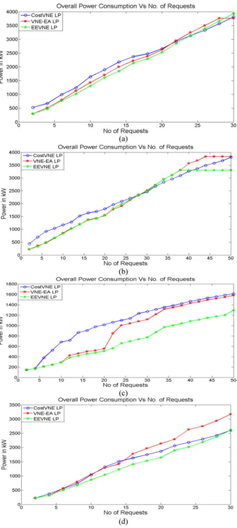
[image:10.594.318.534.274.375.2]Fig. 13. (a) Power consumption under a load of high bandwidth and high CPU demands (Load 1), (b) power consumption under a load of high bandwidth and low CPU demands (Load 2), (c) power consumption under a load of low bandwidth and low CPU demands (Load 3), (d) power consumption under a load of low bandwidth high CPU demands (load 4).
[image:11.594.311.549.64.200.2]Fig. 13 shows the overall power consumption of the different models under the different load conditions of Table II. Fig. 13(a) shows the performance of the different models under Load 1 (high bandwidth and high CPU demands). At this load, the high CPU demands overwhelm the CPU resources of the data centers allowing the substrate network to only accommodate a maximum 30 VNRs out of 50 as will be seen in Fig. 14. The
Fig. 14. Number of accepted requests at various loads. The loads refer to those in Table IV.
EEVNE model outperformed the other models up to a load of 22 VNRs. However, as the load on data centers approaches their full capacity, the CostVNE model starts to perform better as no further savings can be acquired by consolidating resources in data centers and the model with higher savings in the network, in this case the CostVNE model, will have the minimum power consumption.
Fig. 13(b) shows the performance under high bandwidth and low CPU demands. As the links are readily used up to support the high bandwidth demands, the EEVNE model loses its advan-tage over the VNE-EA model as the bandwidth demands will be routed through routes of more hops. The CostVNE model eventually starts to perform better than both the VNE-EA and EEVNE models. The higher propensity of the VNE-EA and EEVNE models to consolidate resources in data centers for minimal power consumption depletes network resources result-ing in future requests beresult-ing embedded far away and thus in-creasing network power consumption. Notice that this happens as requests are served sequentially and the new requests are ac-commodated in the spare capacity. If the network is re-optimized following each new request, the EEVNE model will always be better (or equal to) the CostVNE model. Note that the EEVNE model starts rejecting VNRs earlier than the VNE-EA as it has higher propensity to consolidate resources in data centers.
For request with low bandwidth and low CPU demands (see Fig. 13(c)), the substrate network can successfully accommo-date all the requests as will be seen in Fig 14. The superior performance of the EEVNE model over both the CostVNE and the VNE-EA model is very clear with average power savings of 35% and 23%, respectively as the EEVNE model is able to consolidate resources in data centers and minimize the network power consumption without being restricted by the depletion of the data centers or network resources. Only 30 of the VNRs of low bandwidth and high CPU demands were successfully mapped as seen in Fig. 14. We however still see a superior per-formance in power savings from the EEVNE model over the other two models as shown in Fig. 13(d).
Fig. 15. Energy efficient data center servers power profile.
The VNE-EA model has however only successfully mapped 28 VNRs. This is as a result of the model depleting bandwidth re-sources in the network before even depleting CPU rere-sources in data centers. For Load 2, the load of high bandwidth and low CPU demands, the CostVNE model has successfully mapped all the VNRs but both the VNE-EA and the EEVNE models have fallen short as they have depleted the network resources in order to consolidate resources in data centers. For the load repre-senting low bandwidth and low CPU demands (Load 3), all the three models have successfully mapped all the VNRs because the substrate network has sufficient resources to accommodate them. Finally for Load 4, the load of low bandwidth and high CPU demands, all the three models only successfully map 30 VNRs as they have run out of CPU resources in the data centers.
VI. ENERGYEFFICIENTVIRTUALNETWORKEMBEDDING WITHENERGYEFFICIENTDATACENTERS
In the previous section we evaluated the power consumption of VNE in IP over WDM networks considering energy inef-ficient data centers where unused servers are set to idle state. In this section, we adopt data centers with an energy efficient (EE) power profile where only servers needed to serve a given workload are activated, i.e., unused servers are switched off. The EE power profile is given as a staircase curve as shown in Fig. 15. Considering a large number of data centers as shown by the authors in [37] reduces this relationship between the power consumption and the workload to a linear profile given as:
P Dv ,sb =
μ·CPUv ,sb , if the data centre isON
0, otherwise. (16)
The server power consumption in the data centers is given as
P D= b∈N
v∈V
s∈R
CPUv ,sb ·δbv ,s·μ. (17) Under the EE data center power profile, the EEVNE model no longer seeks the consolidation of data centers as the power consumption of data centers is a function of the workload only not the number of activated data centers. Replacing the data center power consumption in the objective function of the model in Section III by (17) and considering the evaluation scenario in Section V, we evaluate the power consumption of the three VNE models under the energy efficient data center power profile.
Fig. 16. (a) Network power consumption under the EE data center power profile, (b) Data center servers power consumption under EE Data center servers power profile, (c) overall power consumption under EE data center servers power profile, (d) Data center activation under EE data center power profile.
[image:12.594.61.265.68.190.2]account, i.e. the network resource utilization is not restricted by consolidation of resources in data centers. The EEVNE model marginally outperforms the CostVNE model at low loads (not very clear in the figure). This is because in addition to mini-mizing the hop count between nodes chosen for embedding, the EEVNE model tries to minimize the distance between nodes to reduce number of EDFAs. This results in the EEVNE model clustering embedded nodes close to each other and running out of capacity. As a result, future requests are embedded far away thus increasing network power consumption. As such, ignoring distance and concentrating on hop count (number of transpon-ders and routers but not EDFAs) has given the CostVNE model an advantage. As mentioned above, this happens as requests are served sequentially and the new requests are accommodated in the spare capacity. The CostVNE model has maximum power saving of 2% and an average saving of 1% over the EEVNE model, similar to the energy inefficient data center power pro-file results in Fig. 7(a). The EEVNE model however performs better than the VNE-EA model with a maximum saving of 30% and average of 22%.
Fig. 16(b) shows that all the three models have similar power consumption trends in the data centers because the power con-sumption of energy efficient data centers is a function of the workload and not the number of activated data centers as there is no idle power associated with the activation of data centers. Their total power consumption therefore follows the trends of the network power consumption as seen in Fig. 16(c). This leads us to the conclusion that with the energy efficient data center power profile, the optimal VNE approach with the minimum power consumption is the one that only minimizes the number of hops, in this case, the CostVNE model. As mentioned earlier, this is only useful if requests are served sequentially and the new requests are accommodated in the spare capacity.
Fig. 16(d) shows the rate at which all the three models activate data centers with increasing number of VNRs. The CostVNE model has activated all the data centers after embedding the 12th VNR. The EEVNE and VNE-EA models however have a much more gradual activation of data centers which only reaches its peak after embedding the 46th VNR.
VII. LOCATION ANDDELAYCONSTRAINTS
In the previous sections, node embedding was not subject to any location constraints, i.e. nodes could be embedded any-where in the cloud as long as connected nodes of a VNR are not embedded in the same substrate node. In this section we evalu-ate scenarios where the node embedding is subject to location and delay constraints. This scenario represents, for example, an enterprise solution for a service that requires running appli-cations on a virtual machine(s) in a given fixed location (e.g., company headquarter or branch) with one or more redundant virtual machines for protection or load balancing. The virtual machine(s) with a fixed location is referred to as the master node and the redundant virtual machines are referred to as the slave nodes. Such VNRs typically form star topologies with the mas-ter node at the cenmas-ter. The slave nodes can be located anywhere in the cloud subject to delay constraints between them and the
master node in addition to the bandwidth capacity constraints. Depending on the service level agreement (SLA), the redun-dant virtual machine can be located in the same data center but in different racks or full geographical redundancy can be sup-ported by locating each virtual machine in a different substrate node. Locating all the nodes of a VNR in one substrate node eliminates the need for network connections and therefore re-duces the network power consumption and allows the service provider to charge the clients less. On the other hand the cost increases with the provision of full geographical redundancy. In the following results we investigate the impact of different redundancy formats on the power consumption by defining the node consolidation factor (α) as a measure of how many nodes of a VNR can be embedded in the same substrate node. For α= 1, the model only allows one virtual node from the same request to be embedded in the same substrate node while for α= 5, the model allows 5 virtual nodes from the same request to be embedded in the same substrate node.
A. MILP Model With Location and Delay Constraints
We extend the model in Section III, to introduce location and delay constrains. In addition to the sets, parameters and variables defined in Section III-B, we define the following parameters and variables:
Parameters: LOCv
b LOCbv = 1if the master node of VNR v must be
lo-cated at substrate node b, otherwiseLOCv b = 0;
DELv The threshold propagation delay on the links of request
v;
α Node consolidation factor;
∇m ,n Propagation delay on the physical linkm, n, given as:
∇m ,n =3Dm , n
2C , where C is the speed of light.
Variables:
Zm ,nv ,b,e Zm ,nv ,b,e = 1 if the IP over WDM virtual link (b, e) of
VNR v traverses the physical link (m, n), otherwise Zv ,b,e
m ,n = 0.
In addition to constraints (2)–(14) presented in the model in Section III-B, the following constraints are introduced:
δbv ,1= LOCvb ∀v∈V, b∈N (18)
s∈R
δbv ,s≤α∀v∈V, b∈N (19)
n∈Nm
Zm ,nv ,b,e≤1
∀v∈V, b∈N, e∈N, m∈N :b=e (20)
m∈N
n∈Nm
Zm ,nv ,b,e· ∇m ,n ≤DELv
[image:13.594.357.556.528.670.2]that the propagation delay of the virtual links does not exceed the delay threshold.
B. MILP Model Results and Analysis
The NSFNET network is also considered as the substrate network to evaluate the energy efficient VNE with delay and location constraints. We consider a scenario where 15 VNRs for the service discussed above are embedded in the substrate net-work. The number of nodes in the request range between 2 and 5. The propagation delay threshold of the 15 requests is uniformly distributed between 7.5 ms and 75 ms. This range adequately covers the tolerable propagation delay in most applications [38]. The five most populated cities (nodes) in the NSFNET net-work are selected to be the location of master nodes of the VNRs. The concentration of master nodes on a substrate node is proportional to its population. The master nodes in a set of 15 requests are distributed as follows: Houston Texas (Node 6) can host a maximum of 5 master nodes of the set of 15 requests, San Diego (Node 3) can host 4, and Pittsburg (Node 9), Seattle (Node 2) and Atlanta (Node 10) can each host 2 master nodes.
The power consumption of embedding the 15 VNRs is eval-uated versus an increasing CPU and bandwidth load. The range of loads considered is shown in Table III represented by the numbers {1, 2, 3, 4, 5, 6, 7 and 8}. The CPU load is related to the bandwidth requirement according to the assumption that a server working at its maximum CPU utilizes 1 Gb/s of its network resources. Therefore a data center of 500 servers with a 2% workload will generate 10 Gb/s of traffic. This scenario depicts applications whose networking requirements vary pro-portionally to CPU processing requirements. Examples include online video gaming and augmented reality applications for live video streaming for sports. In the following results we compare the energy efficiency of the CostVNE and EEVNE models, the best performing approaches in the previous section, consider-ing constraints on the virtual nodes location and link delay. We refer to the two models with location and delay constraints as CostVNE-LD and EEVNE-LD. In Fig. 17 we evaluate the net-work power consumption, datacenter power consumption and the overall power consumption, versus the increasing loads in Table IV at1≤α≤M AX, whereM AX= 5.
Fig. 17(a) shows the network power consumption. Atα= 1
each virtual machine of a VNR is embedded in a different sub-strate node which increases network traffic thus allowing the CostVNE-LD model to achieve higher power savings in the network compared to the EEVNE-LD model by efficiently us-ing the network wavelengths when embeddus-ing VNRs. With an increasingα, however, the EEVNE-LD model starts to match the CostVNE-LD model as the network traffic is reduced by embedding more virtual machines of a VNR in the same sub-strate node. The ability of the CostVNE-LD and EEVNE-LD to embed all the virtual machines of a VNR in one substrate node atα= 5allows them to minimize the network power consump-tion to zero at load 1. As the load increases the CPU resources become insufficient to embed all the virtual machines of each VNR in one substrate node thus virtual links have to be estab-lished between data centers thus increasing the network power consumption.
Fig. 17. (a) Network power consumption at various values ofα, (b) Data center power consumption at various values ofα. (c) Overall power consumption at various values ofα.
In Fig. 17(b), we extend the analysis to power savings in the data centers. The virtual machine location constraints do not stop the EEVNE-LD model from efficiently consolidating CPU resources and maintaining the same power consumption in data centers asαincreases. This is because the EEVNE-LD model manages to efficiently consolidate virtual machines of different requests at various values ofα.
Introducing further restrictions on the virtual machine loca-tions has, however, increased the power consumption in data centers for the CostVNE-LD model as more data centers will be activated to embed CPU resources while maintaining the mini-mum network power consumption. The EEVNE-LD model has saved 18% of the data center power consumption atα= 1and 5% atα= 5over the CostVNE-LD model.
[image:14.594.313.539.63.473.2]TABLE IV
CPUANDBANDWIDTHLOADDISTRIBUTION
Load CPU Percentage Workload Distribution Link Bandwidth Distribution
1 1–5% 10–40 Gb/s
2 3–7% 20–50 Gb/s
3 5–9% 30–60 Gb/s
4 7–11% 40–70 Gb/s
5 9–13% 50–80 Gb/s
6 11–15% 60–90 Gb/s
7 13–17% 70–100 Gb/s
8 14–19% 80–110 Gb/s
centers does not change as discussed above. The EEVNE-LD model outperforms the CostVNE-LD model in power consump-tion over all the values ofα. Allowing more virtual machines to be embedded in the same substrate node has resulted in limited power savings. As far as the EEVNE-LD model is concerned, the highest savings in overall power consumption of 10% takes place during the transition fromα= 1toα= 2. The transition fromα= 2toα= 3only gives a saving of 4% and the subse-quent increases inαaccount only for very insignificant power savings. From these results we can therefore conclude that for an infrastructure service provider offering a service such as the one presented here, the option of co-location of virtual machines belonging to the same enterprise customer will save power and subsequently cost less, but will not introduce any additional sav-ings by increasing the number of embedded virtual machines of a VNR to more than 2 in the same data center. The power savings acquired from relaxing the virtual nodes location constraints can guide service providers in cost reductions offered to enterprise customers.
VIII. OPTIMIZATION OFDATACENTERLOCATIONSTAKING INTOACCOUNTVIRTUALNETWORKEMBEDDING
In the previous sections, we have considered situations where each node in the network hosts a small data center that can be activated on demand. However, practical considerations such as infrastructure cost and security may limit the number of data centers in a network. In our previous work in [27], we have studied the optimization of data center locations in IP over WDM networks. Here, we show how VNE can impact the design problem of optimally locating data centers for minimal power consumption in cloud networks. We investigate scenarios with a single data center and multiple data centers.
A. MILP Model for Optimal Data Center Locations in Cloud Networks
We have adapted the model in Section III to solve the design problem of optimally locating data centers in cloud networks. In addition to the sets, parameters and variables defined in Sections III-B and VII-A, we define the following:
Parameters:
N DC The total number of data centers in the network; Cv ,s The number of CPU cores requested at virtual nodes
of VNR v;
γ The power consumption per CPU core embedded in a data center;
Variables:
DPb DPb = 1if substrate nodebis a data center, otherwise
DPb = 0;
Δv ,sb Δv ,sb = 1if virtual node s of VNR v has been embedded at data center node b otherwiseΔv ,sb = 0;
Cb The total number of CPU cores at data centerb;
σbv ,s σbv ,s is the XOR of DPb andδbv ,s, i.e., σ v ,s
b =DPb ⊕
δbv ,s,σv ,sb = 1if eitherDPb orδv ,sb is equal to 1,
other-wiseσbv ,s= 0.
The network power consumption is calculated in the same manner as Section III-B. Note that we do not consider minimiz-ing the power consumption of data centers as only the location of a data center is optimized to minimize the network power consumption. This does not affect the data center size (which is governed by the processing requests made) and consequently its power consumption. The extended model is defined as follows:
Objective:
Minimize the network power consumption given as:
m∈N
n∈Nm
P R·Wm ,n +
m∈N
n∈Nm
P T ·Wm ,n
+
m∈N
n∈Nm
P E·EAm ,n ·Fm ,n
+
m∈N
P Om +
m∈N
PMD·DMm. (22)
In addition to Constraints (3)–(14) defined in Section III-B and Constraint (18) in Section VII-A, the model is subject to the following constraints:
Cb =
v∈V
s∈R
Cv ,s·Δv ,sb ∀b∈N (23) DPb+δbv ,s=2Δ
v ,s b +σ
v ,s
b ∀v∈V, ∀b∈N, ∀s∈R (24)
b∈N
Δv ,sb = 1 ∀v∈V, ∀s∈R (25)
b∈N
DPb = NDC (26)
s∈R
Δv ,sb ≤α ∀v∈V, b∈N. (27)
Constraint (23) replaces Constraint (2) in Section III-B. It calculates the capacity of each data center in terms of the number of cores. Note that since our problem is a design problem, the data centers and links are both un-capacitated. Constraint (24) ensures that virtual machines are embedded in nodes with data centers by implementing the AND operation ofDPb andδbv ,s (DPb+δv ,sb ). Constraint (25) ensures that each virtual machine
is only embedded in a data center once. Constraint (26) gives the number of data centers. Constraint (27) replaces Constraint (19) in Section VII-A.
Fig. 18. NSFNET with population percentage information.
in the router ports is modelled as follows:
i∈N
j∈N:j=N
P R·Ci,j. (28)
As such, the objective function becomes:
Minimize the network power consumption given as:
i∈N
j∈N:j=i
P R·Ci,j+
m∈N
n∈Nm
P T ·Wm ,n
+
m∈N
n∈Nm
P E·EAm ,n·Fm ,n +
m∈N
P Om
+
m∈N
PMD·DMm.
B. MILP Model Results and Analysis
The NSFNET network is also used as the substrate network to evaluate the performance of the data center locations opti-mization model. We investigate a scenario where the client’s entry point in the network is fixed but virtual machines could be embedded anywhere and virtual links may also be requested to connect virtual machines. The concentration of enterprise clients in a substrate node is based on the population of the states where the cities (nodes) of the NSFNET network are lo-cated (see Fig. 18). In the case of California where we have two cities in one state (nodes 1 and 3), we have evenly distributed the population of the state between the two cities. We have depicted an enterprise cloud service solution where enterprise clients re-quest virtual machines with a specific number of CPU cores per virtual machine. The power consumption in the data centers is a function of the number of embedded CPU cores. A total of 45 enterprise clients (VNRs) have been considered where the number of virtual machines per enterprise client is uniformly distributed between 1 and 5 and the number of CPU cores re-quired by each machine is uniformly distributed between 1 and 10. The bandwidth requirement of virtual links is uniformly distributed between 10 and 100 Gb/s.
[image:16.594.46.281.68.200.2]We optimized the location of a single data center in the NSFNET network under both non-bypass and bypass ap-proaches. The common practice in 2010 was to locate data centers to minimize cost including the data centers and network
Fig. 19. The network power consumption of a single data center scenario at different locations under non-bypass and bypass approaches.
infrastructure cost and security cost. Considering the cost of the network, the optimal location of the single data center is Node 6. This however also happens to be the optimal location of the data center with the goal of minimizing power consump-tion in the network due to VNE. To verify the results, we ran the model while fixing the location of the data center at the different NSFNET nodes and evaluated the network power consumption as seen in Fig. 19. The model picks a data center such that the embeddings of the virtual machines in the data center will create virtual links that traverse routes with minimal hops. The hop count determines the number of router ports and transpon-ders (the most energy consuming network devices) used under the non-bypass approach. Under the bypass approach, the IP layer is bypassed and therefore the hop count determines only the number of transponders used. Note that selecting a highly populated node and/or a node with highly populated neighbours to locate a data center can significantly reduce the average hop count as more clients are served locally as a result or through a single hop. Therefore the most populous and easily accessi-ble (through minimum hop routes) Node 6 is selected to host the single data center. The optimal location has achieved power savings of 26% and 15% compared to the worst location for the non-bypass and bypass approaches, respectively.
Fig. 20. The network power consumption of a 5 data center scenario under non-bypass and bypass approaches atα= 5.
Fig. 21. The normalized size of five data centers in the optimal locations at α= 5.
[image:17.594.52.552.242.373.2]traversed by low bandwidth demands in order to serve high de-mands locally. The power consumption of transponders used by the selection of routes with higher hop count is compensated by the significant power savings obtained by embedding VNRs of higher bandwidth demands locally. Therefore Node 11 in the optimal data centers locations under the non bypass approach is replaced with the highly populated Node 3 under the bypass approach. The optimal locations have achieved network power savings of 43% and 55% compared to the worst locations for the bypass and non-bypass approaches, respectively. Compared to the single data center solution, distributing the content among multiple data centers has saved 53% and 73% of the network power consumption for bypass and non-bypass, respectively.
Fig. 21 shows the normalized size of optimally located data centers atα= 5. Under non-bypass, the data center located at Node 1 is used to embed the highest number of virtual machines. This is because Node 1 has taken up all the virtual machines of its neighboring populous Node 3 due to the distance between Node 1 and Node 3 being much shorter than the distance between Node 3 and Node 6. Under the bypass approach, a data center is created at Node 3 instead of Node 11. This has significantly reduced the number of virtual machines served by the data center at Node 1 and increased the size of the data center at Node 9 as it has taken up all the virtual machines served by the data center at Node 11 under the non-bypass routing approach.
We have also investigated optimizing the location of data centers in a scenario with geographical redundancy constraints
Fig. 22. The network power consumption of a data center scenario under non-bypass and bypass approaches atα= 1.
Fig. 23. The normalized size of a five data centers in the optimal locations at α= 1.
where virtual machines that belong to the same client cannot be embedded in the same data center (α= 1), i.e., a client re-questing five virtual machines will have one embedded in each of the five data centers. The optimal locations of the five data centers as obtained from the model are (3, 6, 7, 13, and 14) for both non-bypass and bypass. As discussed above the selection of a location to host a data center is governed by two fac-tors: the average hop count between the data centers and clients and the client population of the candidate node and its neigh-bors. In this scenario where virtual machines of the same client cannot be collocated, the model will also try to minimize the hop count between data centers. Fig. 22 compares the network power consumption of embedding the VNRs under the optimal data center locations to the other random data center locations for both non-bypass and bypass approaches. The optimal loca-tions have achieved power savings of 19% and 2% compared to the worst locations for the non-bypass and bypass approaches, respectively.
[image:17.594.48.309.247.376.2]