Causality of Optimized Haskell: What is burning our cycles?

promoting access to White Rose research papers

White Rose Research Online

[email protected]

Universities of Leeds, Sheffield and York

http://eprints.whiterose.ac.uk/

This is an author produced version of a paper published in

Proc. ACM

Symposium on Haskell

White Rose Research Online URL for this paper:

http://eprints.whiterose.ac.uk/id/eprint/77401

Paper:

Wortmann, PM and Duke, DJ (2013)

Causality of Optimized Haskell: What is

burning our cycles?

In: Proc. ACM Symposium on Haskell. ACM Haskell

Symposium 2013, 23 - 24 Sep 2013, Boston, MA, USA. ACM Press , 141 - 151.

Causality of Optimized Haskell

What is burning our cycles?

Peter M Wortmann

David Duke

University of Leeds

{scpmw,d.j.duke}@leeds.ac.uk

Abstract

Profiling real-world Haskell programs is hard, as compiler opti-mizations make it tricky to establish causality between the source code and program behavior. In this paper we attack the root issue by performing a causality analysis of functional programs under optimization. We apply our findings to build a novel profiling in-frastructure on top of the Glasgow Haskell Compiler, allowing for performance analysis even of aggressively optimized programs.

Categories and Subject Descriptors D.2.5 [Software Engineer-ing]: Testing and Debugging—Debugging Aids; F.3.2 [Logics and Meanings of Programs]: Semantics of Programming Languages— Operational semantics

Keywords Profiling; Optimization; Haskell; Causality

1.

Introduction

A major selling point of functional languages is their clean model of computation, prioritizing ease of composition over efficient map-ping to hardware. By strictly dividing up responsibilities, aggressive compiler optimizations can then often close the gap again. Unfortu-nately, this also makes it hard to reason about compilation process: Where a performance problem ends up falling through the cracks, it often becomes exceptionally hard to explain. Therefore we need specialized profiling tools to assist the programmer in pin-pointing the performance problems and explaining the root causes behind them. These tools must bridge the full abstraction gulf, accurately measuring low level performance while relating it all the way back to the original source code.

1.1 Context

The ecosystem of real world Haskell development currently centers mostly around the Glasgow Haskell Compiler GHC [19]. And this for good reason, as it is has managed to make extensive optimization techniques such as heavy in-lining [18], rules [4, 22] and lax code-reordering [17] relevant to everyday programming tasks. This has

∗_{This work was kindly supported by Microsoft Research through its PhD} Scholarship Programme.

Permission to make digital or hard copies of all or part of this work for personal or classroom use is granted without fee provided that copies are not made or distributed for profit or commercial advantage and that copies bear this notice and the full citation on the first page. Copyrights for components of this work owned by others than the author(s) must be honored. Abstracting with credit is permitted. To copy otherwise, or republish, to post on servers or to redistribute to lists, requires prior specific permission and/or a fee. Request permissions from [email protected].

Haskell ’13, September 23–24, 2013, Boston, MA, USA.

Copyright is held by the owner/author(s). Publication rights licensed to ACM. ACM 978-1-4503-2383-3/13/09. . . $15.00.

http://dx.doi.org/10.1145/2503778.2503788

enabled Haskell programs to perform competitively even while taking full advantage of the language’s abstraction mechanisms.

However, there have been common complaints that the perfor-mance of Haskell programs can be quite unpredictable [28]. And while there has been a robust and well-tested profiling framework for the GHC compiler for some years now [25], it has to impose significant restrictions on what optimizations the compiler is al-lowed to perform. Furthermore, newer work [14] suggests that its cost attribution scheme still has room for improvement.

1.2 Motivation

Consider the following popular example program in Haskell:

f a c : : I n t → I n t

f a c n = f o l d r _{( * ) 1 [ 1 . . n ]}

We compute the factorial of a numbernby multiplying out the numbers from1ton. What performance would we expect?

The answer is surprisingly complicated, even for this simple program using common library functions. If we compile with GHC, we have to account amongst others for specialization, inlining, short-cut deforestration [7], strictness analysis as well as the worker-wrapper transformation [5]. After many steps, these transformations strip our function down to its core loop:

go !w ! n | w == n = w

| o t h e r w i s e _{= w * go (w+1) n}

This is remarkable – yet for large inputs the optimized codestill

runs out of stack space needlessly, as it was not constructed to be tail-recursive! To make matters worse, conventional profiling would be useless here, as it would either prevent key optimizations from happening – or present information so coarsely that we would have to guess at what is happening in the inner loop.

1.3 Contribution

We have built a profiling framework that is able to handle profiling even for such tricky interactions between various code pieces and compiler optimizations. This is fundamentally about balancing two concerns: Accurate tracking of causes for performance problems, and feasibility of actual instrumentation and profile analysis.

We will attack these separately: In Section 2 we will explain our causality model and apply it to derive exact cause-effect relations for the evaluation of a simple lazy functional language. In Section 3 we will then show how we can extend the approach to reason about compiler optimizations as well.

2.

Tracking Causality

In profiling, we are ultimately looking for explanations:Whydid this performance problem occur? This invariably leads to deeper questions: Why did the machine behave like that? Where exactly was that call coming from? What made the compiler generate the code in that way? The answers to these questions make up the actual

causalstory behind the performance of the program.

In this section we will start out by showing how we can find such answers for a simplified lazy functional language. The idea is that we track thecausefor every piece of code, value or run-time cost. As long as we make sure that we identify causality correctly at every step along the data flow, this promises us profiles that are correct by construction.

2.1 Counter-Factual Causation

In order to formally reason about causality, we need a causality model. Our goal is to be able to support claims such as:

Usingfoldrhere causes excessive stack usage.

How would we show such a statement to be true? Let us negate both sides to getcounter-factualconditionals [13]:

Notusingfoldrhere can cause less stack usage. This we can actually somewhat test: If we could show that similar programswithoutfoldrlack the original problem, we have indeed demonstrated a causal connection. This approach forms the basis of Lewis’ classic theory of counter-factual causality [13].

To put this formally, let us call the original program and its behavior a “world”W. Then if we have a causeα(using foldr) and effectω(stack usage) that are true inW, we are allowed to derive the counter-factual causation relation

¬α→ ¬ω

if and only if theclosestworldW0whereαwould be false would

alsoseeβbecoming false.

Perhaps surprisingly, Lewis theory leaves it almost completely open what the “closest” world should be – it is a parameter that has to be set intuitively based on the problem at hand. In our case, this means we first need to define how to reason about programs and their execution! In the following we will continue to notate causes asα, β,γandδ, and useαβ=α∧βfor a cause conjunction.

2.2 Definitions

Let us define a simple cause-annotated lazy functional language to continue our discussion. We will notate variables as xor y, constructors asCorD, values asvand expressions ase:

v ::= C x1x2...

| λy.e | ⊥ e ::= v

| e x | x

| let{x1=e1, x2=e2, . . .}ine

| caseeof{C x1x2...→e1;D y1y2...→e2;. . .} wheree=hαieis an expressionannotatedwith its causeα. By this we mean that if we haveβas the event of encounteringhαie, we have¬α→ ¬β: ifαbecomes false, it might causeeto change.

To reason about performance, we introduce cost termsO:

O ::= L | C | A | V | T | E | ⊥

with each unit of abstract cost corresponding to an application of a rule from the language semantics we are about to define. For

example each evaluation of aletexpression should produce one unit ofT cost. Cost annotations will have the same meaning as on expressions, but use the slightly more compact notationO=αO. We define profilesθ=αO1+βO2+· · · as bags of such cause-annotated costs.

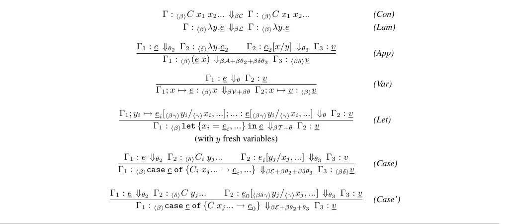
At this point we have enough to consider evaluation semantics. We will use Launchbury’s natural semantics for lazy evaluation [12] as our starting point, but extend it with annotations and profiles. Our judgments will take the following form:

Γ :hβie ⇓θ Γ0:hγiv

WithΓstanding for the heap (a variable mapx7→ e;...) before evaluation andhβiethe annotated expression to evaluate. On the right side the judgment yields the profileθ, a new heapΓ0 and an annotated result valuehγiv. The profile notation was inspired by Launchbury as well as Sansom et al [25]. As usual, where a judgment can not be derived (finitely) from the semantics, the judgment result are⊥terms.

2.3 Deriving Annotations

Consider the application rule:

Γ1:e ⇓θ2 Γ2 :hδiλy.e2 Γ2:e2[x/y] ⇓θ3 Γ3:v

Γ1: hβi(e x) ⇓?A+?θ2+?θ3 Γ3:h?iv

So far this is just Launchbury’s rule with annotations and profiles added where syntactically required. Unfortunately it is not quite immediately obvious how we should annotate: Do we need extra annotations onv, and what about the various costs in the generated profile? We must consult our causality model and derive causes from the terms the rule match depends on (highlighted).

First consider the application expression(e x). To find its effects, our causality model says that we need to consider an alternate world

W0 where(e x)was “miraculously” replaced with a differente0

just as we were about to apply the rule. Let us picke0=⊥as our replacement. As no rule is allowed to match⊥, this would lead to the followingW0judgment:

Γ1 :⊥ ⇓⊥ ⊥

We observe that inW0 the judgment does not generatevor any of the costs in question. We can therefore conclude that they were caused by encountering(e x)and therefore – by transitivity – byβ. Hence we must annotateβon all costs in the profile as well as on the return value.

Let us repeat this procedure with the result of the evaluation ofe, which the rule expects to behδiλy.e2. Again we ask: What if in an alternate worldW00we switched out the returned value bye00=⊥? By matching as far as possible1we obtain theW00judgment

Γ1:e ⇓θ2 Γ2:⊥

Γ1:hβi(e x) ⇓βA+βθ2+β⊥ hβi⊥

Accordingly, it follows that we need to annotate the profile θ3 as well as the return value v. We arrive at the fully annotated application rule:

Γ1:e ⇓θ2 Γ2:hδiλy.e2 Γ2:e2[x/y] ⇓θ3 Γ3:v

Γ1:hβi(e x) ⇓βA+βθ2+βδθ3 Γ3:hβδiv

Note that we completely ignore heaps where the result was⊥, even though alternate worlds would probably also update the heap differently! This is because we have to think of expressions and values as graphs and our rules as graph reductions: a free variable is actually a place-holder for a shared expression or value from the heap. Consequently, the heap state does not matter without a reference to it.

Γ :hβiC x1x2...⇓βC Γ :hβiC x1x2... (Con)

Γ :hβiλy.e ⇓βL Γ :hβiλy.e (Lam)

Γ1:e ⇓θ2 Γ2:hδiλy.e2 Γ2 :e2[x/y] ⇓θ3 Γ3:v

Γ1:hβi(e x) ⇓βA+βθ2+βδθ3 Γ3:hβδiv

(App)

Γ1:e ⇓θ Γ2:v

Γ1;x7→e:hβix ⇓βV+βθ Γ2;x7→v:hβiv

(Var)

Γ1;yi7→ei[hβγiyi/hγixi, ...];...:e[hβγiyi/hγixi, ...] ⇓θ Γ2:v

Γ1:hβilet{xi=ei, ...}ine ⇓βT+θ Γ2:v

(Let)

(withyfresh variables)

Γ1:e ⇓θ2 Γ2:hδiCiyj... Γ2:ei[yj/xj, ...] ⇓θ3 Γ3:v

Γ1:hβicaseeof{Cixj...→ei, ...} ⇓βE+βθ2+βδθ3 Γ3:hβδiv

(Case)

Γ1:e ⇓θ2 Γ2:hδiC yj... Γ2:e0[hβδγiyj/hγixj, ...] ⇓θ3 Γ3:v

Γ1:hβicaseeof{C xj...→e0} ⇓βE+βθ2+θ3 Γ3:v

(Case’)

Figure 1. Annotated evaluation rules

2.4 Advanced Annotations

In the last section, our recipe for removing expressions in the alternate world was to replace them bye0 = ⊥. On one hand, this is very effective, as it clearly removes any trace of the original expression. On the other hand, it always forced an immediate rule mismatch, which is rather crude. After all, Lewis’ theory suggests comparing to a world that is ascloseas possible to the original.

Consider for example the Sestoft-styleletrule [26]:

Γ1;yi7→e_i[yi/xi, ...];...:eB[yi/xi, ...] ⇓θ Γ2:v

Γ1: hβilet{xi=ei, ...}ine B _⇓

?T+?θ Γ2:h?iv Here the evaluated expression is the only interesting input term. If we again sete0=⊥we would obtain the following annotated rule:

Γ1;yi7→e_i[yi/xi, ...];...:eB[yi/xi, ...] ⇓θ Γ2:v

Γ1:hβilet{xi=e_i, ...}ineB ⇓βT+βθ Γ2:hβiv with annotations both on all costs as well as the returned value. However, this result might sound a bit suspicious: The role of a

letexpression is to add bindings, not influence control flow or the result of the evaluation of the body. From this point of view, the annotations onθandvlook a bit shaky.

Can this intuition be supported formally? If we were right, we would have to find another worldW00where theletexpression was gone, but the costs as well as the result of the body’s evaluation would still appear. Well, let us try to simply sete00=eB! In the unlikely case that evaluation of the naked body happens to never use the now-undefinedxivariables, this would allow the following

W00judgment:

Γ1 :eB ⇓θ Γ2:v

Which would indeed be the sameθandvthat we originally obtained. This in turn would mean that we would not have to annotate either, matching the intuition of not seeing them as directly influenced by theletexpression!

2.5 Binding Effects

We seem to be going into the right direction: Simply by changing the alternate expression under consideration we have identified a case where we can safely reduce the amount of annotation. On

the other hand, we can obviously not simply ignore the possibility thatlet-bound variables might be in use. Launchbury defines three rules where bindings influence program evaluation:

1. The variable rule, which would fail to look upxion the heap.

2. The constructor rule, which might produce a constructor men-tioningxiinstead ofyi.

3. The application rule, which could sub-evaluate an expression usingxiinstead ofyi

We see that all three rules can be expected to produce different results where they use the eliminatedxibindings. Therefore we

want their result terms to get annotated.

We can achieve this using a trick: If we look ahead to Figure 1, we see that all three rules add their expression annotation to their results. Therefore, we can simply have the annotatedlet-rule add the annotations on the affectedexpressions:

Γ1;yi7→e_i[hβγiyi/hγixi, ...];...:e[hβγiyi/hγixi, ...] ⇓θ Γ2:v

Γ1:hβilet{xi=ei, ...}ine ⇓βT+θ Γ2:v

whereei[hβγiyi/hγixi]is a replacement rule updating the variable name as well as the annotation on the expression directly containing it. This way ensures indirectly that any (potentially) differing result will be annotated with the cause of theletexpression.

2.6 Assembling

We see that a smart choice for the “closest world” can lead to more specific annotations. However, as the last subsection should have demonstrated, actually finding ways of getting the right annotations is not always trivial. As a compromise between accuracy and resulting annotations rule complexity, we will from here on use the following alternate world rule for removing an expressione:

e0=

8 > > > <

> > > :

eB

ife=let{...}ineB

eB

ife=case...of˘...→eB¯

witheB

sole branch

⊥ otherwise

comes with just one extra subtlety: The removal might skip a non-terminating scrutinee computation, a change that strictly speaking would require an annotation. However, note that the object of an-notation would be a profile or value that in W would never be produced in the first place, therefore this is inconsequential for pro-filing. Annotating all remaining rules accordingly, we finally arrive at the rule set laid out in Figure 1.

3.

Optimizations

At this point we can derive program behavior and profiles for anno-tated programs in our toy language. With this we could, for example, already de-sugar a higher level language into our representation and derive meaningful profiles.

However in real-world situations we will rarely want to execute a program exactly as it was written. Compiler optimizations allow more flexibility for the programmer in how to write the program, by taking advantage of functionality-preserving transformations that are expected to improve program performance.

Optimizations pose a special challenge for tracking causality: While such transformations will often radically change how the program looks and executes at the point of optimization, in the end we are still bound to arrive at the same values and cost profiles with only a few local changes. For our analysis this means that just looking at the transformation in isolation would be short-sighted. Instead we must look all the way through evaluation and consider what effect the transformation has on the costs of the evaluation of thefull program. Then we can again derive annotations, this time using the behavior of the unoptimized program as the “closest world” point of comparison.

3.1 Beta Reduction

Assume we have a situation where the function expression of an application is a lambda. We can then optimize the expression by eliminating both the application and the lambda expression using beta reduction. The rule could look like follows:

hβ1i

`

hβ2iλx.e

´

y =⇒ h?ie[y/x]

To derive the annotation, we compare the behavior of the unop-timized version (W) with the optimized one (W0). Plugging the original expression into the semantics from Figure 1, we derive for

W:

Γ :hβ2iλx.e ⇓β2L Γ :hβ2iλx.e Γ :e[y/x] ⇓θ Γ 0

:v

Γ :hβ1i

`

hβ2iλx.e

´

y ⇓β1A+β1β2L+β1β2θ Γ 0_:

hβ1β2iv This looks promising: In both worlds we end up evaluatinge[x/y]. Moreover, both the result valuevand the profileθgain just anβ1β2 annotation inW. So we just have to make sure all costs generated bye[x/y]get aβ1β2annotation inW0and the difference of the profiles will be exactly the optimized-out costsA+L!

Unfortunately, we can not quite achieve this by adding a simple

β1β2 annotation on the right side of the optimization rule. After all we have to account forletand one-branchcaseexpressions, which as explained in Section 2.4 do not add their expression cause to all their results. Yet we can still achieve the desired effect by “pushing” the annotation inwards on these occasions:

hhαiie=

8 > > > > > <

> > > > > :

hβilet{...}inhhαiie0

ife=hβilet{...}ine0 hβicase...of

˘

C0...→hhαiie0

¯

ife=hβicase...of{C0...→e0} hαie otherwise

For which we now can easily see that:

Γ :e ⇓θ Γ

0

:v ⇒ Γ :hhαiie ⇓αθ Γ

0

:hαiv

And therefore re-state the beta reduction rule as:

hβ1i

`

hβ2iλx.e

´

y =⇒ hhβ1β2iie[y/x]

In the end, let us reiterate that our approach lead to theexactsame profile – minus the cost for the sub-expressions that was optimized out. Clearly it is not impossible to rework the program significantly without reducing the profile quality.

3.2 General Case

Consider the evaluation of an arbitrary expressionethat was trans-formed toe0=opt(e)by an optimization:

Γ1:e ⇓θ Γ2:hβiv ⇒ Γ1:opt(e) ⇓θ0 Γ0₂:_hβ0_iv

As long as the optimization is correct, we know that we have to arrive at the same result value v once we have evaluated it to normal form by resolving all referenced thunks. Given that most optimizations are local improvements, we would also expect a lot of costs to appear in bothθas well asθ0. As we only have to account for effects that actually change, this means that we do not have to reconsider their causes: The annotation rule should attempt to match them and ideally arrange for the annotations to stay the same after transformation. On the other hand, there are some cases where we have to allow changes to the profile. We will explain the interesting cases in the following subsections.

3.2.1 Preemption

In some situations, preemption might make it impossible to actually retain the same annotations. Consider the example:

let{x=... , y=hαicasexof...}in... x ... y ... Will the cost for evaluatingxbe annotated withα? Obviously, this depends on whetherxorywill end up getting evaluated first. Now suppose we have an optimization that changes the order in whichx

andyget evaluated: Should we require that it somehow retains or suppresses theαannotation on the costs for evaluatingx?

This however would be very hard to achieve in this case. Luckily, we can argue that it is not actually required: We can see the different possible causes for the evaluation ofxaspreemptingeach other. Either of them would be a sufficient cause, it just so happens that only one of them can actually occur in any given program execution. Therefore causes that preempt each other are interchangeable in our analysis, and we can allow optimizations to freely substitute them with each other.

3.2.2 Overheads

Furthermore, sometimes optimizations might not just remove or reorganize costs, but actually introducenewcosts. Such overheads might for example happen where an optimization rule replaces one cost type by another: We would see it as optimizing out one cost and introducing the new one as overhead.

This constitutes an actual alternate world change, with the trans-formation as its cause. Therefore our causality model demands annotating such effects with the transformation cause. For typi-cal transformation rules, this will be the annotations of the sub-expressions that the transformation matches on, such asβ1β2 in Section 3.1.

3.2.3 Annotation Overreach

Γ :hα1icasee1of

˘

C x→hα2ilet{y=e2}ine3, ...

¯

"

Γ :e₁

⇓θ1 Γ1:hδiCxˆ

2

6 6 6 6 4

Γ1:hα2ilet{y=e2}ine3[hα1δγix/ˆ hγix]

"

Γ1; ˆy7→ˆe2: ˆe3[hα1δγix/ˆ hγix]

⇓θ2 Γ2:v

⇓α2T+θ2 Γ2:v

⇓α1E+α1δα2T+α1θ1+α1δθ2 Γ2:hα1iv

`

withˆe=e[hα2γiy/ˆ hγiy]

´

Γ :hβ2ilet{y=e2}in

`

hβ1icasee1of{C x→e3, ...}

´

2

6 6 6 6 6 6 6 6 6 6 4

Γ; ˆy7→ˆe₂ :hβ1icasee1of{C x→ˆe3, ...}

"

Γ; ˆy7→ˆe₂:e₁

⇓θ1 Γ1; ˆy7→eˆ2:hδiCxˆ

"

Γ1; ˆy7→ˆe2:e3[hβ2γiy/ˆ hγiy][hβ1δγix/ˆ hγix]

⇓θ0

2 Γ2:v 0

⇓β1E+β1θ1+β1δθ02 Γ2:hβ1iv 0

⇓β1E+β2T+β1θ1+β1δθ20 Γ2:hβ1iv 0

`

withˆe=e[hβ2γiy/ˆ hγiy]

´

Figure 2. Evaluation before and after floating optimization

When handling tricky cases, this will end up as our main source for profile degradation, and we will see an example in the next section. Note however that overestimating effects is a common and relatively benign mistake – essentially introducing circumstantial information of little direct relevance into the profile. As long as do not overload the profile with such annotations we can be reasonably sure that it will still have value in performance analysis.

3.3 Floating

Let us test these rules to the “floating” optimization, which relocates bindings within an expression [20]:

hα1icasee1of

˘

C x→hα2ilet{y=e2}ine3, ...

¯

=⇒ hβ2ilet{y=e2}in

`

hβ1icasee1of{C x→e3, ...}

´

Here we are floating theybinding out – for example because we are in the process of promoting it to a statically allocated top-level constant. This is a very common optimization, hence we would like it to have little impact on profile quality. Can we setβ1andβ2in a way that achieves this?

Figure 2 shows the evaluation of both versions under the assump-tion that thee₃branch gets actually taken and all sub-evaluations terminate. Note that the profiles look very similar if we assume

β1 =α1andβ2=α2, mostly thanks to the specialletrules we derived in Section 2.4. However there is one problem with setting

β2this way: TheT cost would lose theα1δannotation.

This is hardly surprising: Clearly the execution of the let

expression used to depend on whatcasebranch was taken, whereas now it gets evaluated unconditionally. How do we handle this? No preemption takes place, and due toδ getting only determined at run-time, we have no way to include it inβ2. The only option left is therefore to seeT as first optimized out, then re-introduced again as anoverhead. This shifts its cause to the transformation, and makes it valid to annotate it withβ2=α1α2:

θ=α1E +α1δα2T +α1θ1 +α1δθ2

⇓ (remove) (new) ⇓ ⇓

θ0=α1E +α1α2T +α1θ1 +α1δθ20

However, we are still not quite finished: Note thatβ2gets inserted intoe₃via substitution, therefore potentially propagating the extra

α1annotation intoθ0andv0– an instance of annotation overreach. Yet note that this does no actual harm, as both terms get annotated withβ1 = α1 by thecaserule anyway, and we actually know thatα1θ2 = α1θ02. So in the end the only difference betweenθ andθ0will be that theα1δannotation onT gets replaced byα1α2, truthfully reflecting exactly the relocation of theletexpression.

3.4 Arbitrary Optimizations

At this point we have shown that our system is flexible enough to accommodate two transformations commonly used in optimization. But what can we find a way to satisfy the requirements from Sec-tion 3.2 no matter what the optimizaSec-tion rule is? This is interesting as we would ideally like to support programmer-supplied optimiza-tion rules [22] that are allowed to make almost arbitrary program modifications.

Consider the basic short-cut list fusion rule from the cited paper:

{−#RULES“foldr/build”

∀kz(g::∀b.(a→b→b)→b→b).

hαifoldrk z(hβibuildg) =hαβig k z#−} The idea here is thatk andz encode a way to consume a list, whilegdescribes how the list should be built. The rule says that whenever we find them combined in this way, we can just eliminate the immediate list and construct the result directly.

For the profile, this is a dangerous change: Just from the rule, we know very little about its cost implications. We can just estimate them to be substantial, given that we eliminate calls to two non-trivial functions. Saying more would require deep analysis of the reasoning behind the rule, which is a task that the compiler cannot perform automatically. Therefore we have to either ask the rule writer to provide the proper annotation method for us, or find a way to annotate that requires no further knowledge about the rule.

In the last section we have already seen how we can handle cost changes that we fail to map cleanly: We simply declare them as being removed, then being re-created by the transformation as overheads. In our case, the most conservative annotation strategy is therefore to see this as happening forallcosts touched by the optimization. Fortunately, in a pure language we know these to be exactly the returned profile and result value, therefore forcing annotations on these two terms should yield a valid program profile. As shown in Section 3.1, we can achieve this using a push annotation. In general, if we have an optimizationopt that gets triggered by an eventαβ(as above), it is always correct to annotate:

hαi...e1...hβi...e2 =⇒ hhαβ...iiopt(e1, e2)

Note that for unmatched sub-expressionse_i we do not need to touch annotations, as the rule application does not depend on them. As a result, while this is the most conservative choice, we still end up with fairly non-intrusive annotations. In the example of thefoldr/buildrule, it is actually easy to see that this is the only valid choice. Paired with the fact that such specialized rules generally are not applied very often compared with, say,let

hαilet{f=..., g=...,

h=hγicaseyof{C1x→f, C2x→g}}

in hβih x

f=..., g=...

h=hγi...

in hβih x lexical

evaluation value

value

Figure 3. Scopes for an application expression

4.

Profiling Design

Up to this point, we have only considered what cost causes would be if assigned by a perfect outside observer with limitless memory. This is the appropriate viewpoint to take while compiling and optimizing source code, as there is no good reason to sacrifice diagnostic power at that point. However once we deal with an actual running program, cost analysis and attribution has a tricky problem: If measurements consume significant resources itself, it will skew the very results we are interested in! In practice, this means that we

mustreduce the amount of causes we track if we want to produce useful results.

This section will investigate the design space, outlining different ways we can cut down on the amount of information gathered. We will use this occasion to discuss other profiling frameworks and evaluate their design decisions.

4.1 Prioritization

If we have to drop annotations, which ones should we choose? Observe that cause annotations vary in usefulness: For example,

everycost will causally depend on the evaluation of the entry point “main”. Therefore unless the performance problem resided exactly in this function, this lead would be pretty useless while tracking down a performance problem.

We therefore postulate that some causes are more closely cou-pled to an effect than others: The fewer other effects a cause has, the more likely it is to be the root of the problem. We even have a way to reason about this from our semantics: Note that outer rule applications generally add annotations toallcosts that are produced by nested rule applications. Therefore outer rules annotate strictly

moreeffects and are therefore less specific.

This “ranking” of causes is very commonly exploited by pro-filing frameworks to cut down the amount of information to track, while at the same time structuring it for easier analysis. For example the original profiling solution proposed by Sansom et al [25] only ever tracks the upper-most cost-centre. Other implementations track cause terms as stacks, as for examplegprof[8] or newer imple-mentations of cost-centre profiling [24]. This practice is especially prevalent in profiling tools for imperative languages, as call stacks are relatively stable there.

Note however that this is generally not the case for optimized purely functional programs. In fact we made no attempts whatsoever so far to ensure stack consistency or annotation order, in contrast to Sansom’s work. This is a deliberate, as we see no way to maintain stack consistency while allowing enough freedom for optimizations.

4.2 Value Annotations

Our semantics annotate every value with its full causal history. As there is no way to predict the annotations statically, a direct implementation would have to store and dynamically compose causes at run-time. This however would come at considerable cost, as programs typically process large amounts of data. Tracking every value would increase memory access and consumption significantly. Figure 1 also tells us that there are merely two rules where value

annotations make their way into the profile:(App)and(Case)– unsurprisingly the two points where control flow depends on values. The most common simplification is to skip value annotations in the(Case)rule, which allows ignoring annotations on all non-lambda values at run-time. This helps a lot, as non-non-lambda values can be expected to make up most of the run-time data. And while it is entirely possible to encode program behavior as data, primitive or constructor values rarely end up being the most interesting influence on program performance.

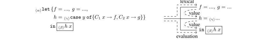
4.3 Lambda Annotations

Lambda values, on the other hand, need more consideration. It is characteristic for the functional style to not only control execution by calling functions, but also bypassingfunctions to be called by other code, for example when using monads [29]. Therefore, both the origin of the lambda as well as the application site might turn out to be a fruitful lines of inquiry for solving a performance problem. For example in Figure 3 we should get the fullαβγannotation on costs coming fromf org. However implementing this would be expensive, as there is no cheap way forhto update the annotation of the closure as it gets passed through.

To solve this, Sansom et al track only the cause of the lambda allocation, thelexical scopeα. The advantage of this approach is that the allocation site is constant for any closure object on the heap, and therefore does not need to be updated. This design ignores the cause for the evaluation of the application, a deliberate design choice [24]. However recent work by Marlow [14] concludes that this often leads to misleading cause stacks, and extends Samson’s work by merging lexical and evaluation scope in applications. This would lead to an annotation ofαβin the above example.

Either solution would missγ, which is arguably acceptable for the same reasons that we regard value annotations as less important. Note that cost-centre profiling already has to pay significant over-heads just for tracking evaluation and lexical scopes in this fashion. Most critically, it requires a non-trivial heap layout change, which not only changes the space complexity of the program, but also makes it impossible to use normally compiled code in a program that uses profiling.

4.4 Static Lexical Scope

To get around this, note that we can actually know a good portion of the lexical scope just by looking at the closure identity. Suppose we find out thate₁in the following example was evaluated:

hαilet˘f=hβiλx.e1

¯

ine2

5.

Implementation

At this point we have a solid idea of how we expect the compiler to attribute code with cause terms, and in the last section we out-lined the general trade-offs involved in an implementation. We will now describe our implementation of a new profiling framework for Haskell. In line with the theoretical work, we will focus on allow-ing profilallow-ing of fully optimized programs with high accuracy and minimum overhead. We will especially use zero code instrumenta-tion, basing everything off maps of the generated machine code and non-intrusive run-time system changes.

The reasons for this focus are two-fold: Firstly, the framework by Sansom et al [25] is already well-established for big-picture profiling. But more importantly, modern Haskell usage has shown its great potential for heavy optimization, leading to tight inner loops that require careful performance analysis. We aim to provides useful results even under these demanding circumstances.

5.1 Cause Tracking in Core

Our work is based on the Glasgow Haskell Compiler [19]. The first step in the implementation of a proper profiling framework is to make sure that we can track causes throughout its compilation according to the rules we explained in the first sections.

To make this work, we have to represent cause annotations in every representation the program takes throughout the compilation process. The first stage in the process is that GHC will “de-sugar” full Haskell into a significantly reduced functional language called “Core” [17]. We can use existing facilities [6] at this point to en-sure that every interesting program expression will be annotated with a “ src ” tick expression. For example, the program from the introduction could look like follows after de-sugaring:

f a c n : : I n t → I n t

f a c n =

s r c< f a c . h s : 2 , 1−2 , 2 7 >

f o l d r (s r c< f a c . h s : 2 , 1 5−_{2 , 1 8 > ( * ) )}

(s r c< f a c . h s : 2 , 1 9 > 1 ) (s r c< f a c . h s : 2 , 2 1−2 , 2 7 > [ 1 . . n ] )

Note that in contrast to our syntax from Section 2.2 we now repre-sent causes as anexpressiontype. Additionally, we will actually see them as applying to every profile and value that gets passed through, making their semantics that of the see them as corresponding to the “push” annotations from Section 3.1. These choices make annota-tions fit naturally with the compiler design. For example in-lining “foldr” right away would yield:

f a c n : : I n t → I n t

f a c n =

s r c< f a c . h s : 2 , 1−2 , 2 7 >

s r c< B a s e . l h s : 1 4 , 1−1 7 , 3 6 >

l e t go y s =

s r c< 16 ,13−17 ,36 > c a s e y s o f

[ ] → s r c< B a s e . l h s : 1 6 , 2 5 >

s r c< f a c . h s : 2 , 1 9 > 1 ( y : y s ) → [...]

i n go

This is consistent with our rules. Consider how we would achieve this result: We would first let-bind the parameters to “foldr”, then unfold its definition andβ-reduce it according to Section 3.1. This leads to the double-annotation on the top-level expression.

Second, we would let-float the parameters inwards as described in Section 3.3 until we have reached the usage site. On the way, we do not have to add additional annotations on the expressions we pass, as we established. Only when we unfold the values in question at the usage site we take over the respective annotation, leading to the “inner” annotation on the “1” expression in the example.

5.2 Core Issues

Unfortunately, this mapping is not a perfect implementation of our semantics. While giving annotations “push” semantics makes it more straight-forward to relocate expressions, this means that there is no way of annotatingletor one-branchcaseexpressions themselves. For a more complete solution, we should probably allow attaching ticks individually to these sub-expressions.

On the other hand, note that the interaction between push anno-tations and binding expressions allows us to “float”srcticks easily. This means that we are allowed to optimize ticks like follows:

src<1>let ... in src<2> ...

=⇒ src<1>src<2>let ... in ... By repeating this process, we can limit the places in the expression that we can encounter source ticks, which makes it easier to make sure that we they do not get into the way of GHC’s optimizations.

5.3 Cause Tracking in Cmm

After the Core optimizations have taken place, GHC will translate the Core program into a high-level assembly language called Cmm (related to C--[21]). The inner loop of our factorial function would be implemented by the following annotated Cmm code:

Main . $ w g o _ e n t r y ( ) {

A : s r c< f a c . h s : 5 : 1 5−1 7 > , . . .

c t x<B> c t x<C>

i f ( Sp−16 < SpLim ) g o t o B ; e l s e g o t o C ; B : R1 = Main . $ w g o _ c l o s u r e ;

c a l l s t g _ g c _ f u n ( R2 , R1 ) ; C : c t x<D> c t x<E>

_tmp = R2 ;

i f ( _tmp ! = 2 0 ) g o t o D ; e l s e g o t o E ;

[...]

}

While Cmm borrows conventions from C, it is quite a low-level language. We can see that all code has been broken down into blocks that are jumped to directly – and that the stack check that might eventually cause our program to fail is now spelled out explicitly.

To track source code annotations, we again insert meta-statements that “color” the code following it. However note that in contrast to functional code, Cmm does not have a recursive struc-ture that we can exploit: Without further annotations, it would be unclear whether the source annotation in block A should apply to, for example, block C as well. This is a special instance of the prob-lem mentioned in Section 4.4: We want to be able to follow control flow backwards in order to maximize the annotations we are able to “see”. We solve this by introducing special “context” annotations that declares the containing block to be the static context of the second block, which is therefore allowed to inherit all annotations.

5.4 DWARF

5.5 Sampling

At this point, we have enough information to track any piece of executable code back to at least one position in the source or library code – and typically many more due to inlining, as explained in Section 4.4. This means that all we require in order to profile a program is an approximate map of positions in the executable to costs. The standard process of obtaining such a map is called sampling: We stop the program at periods proportional to its resource usage, and inspect the program state to find clues as to what lead to the resource hunger of the program.

Currently we implement the following sampling methods:

1. By hardware counters: Such counters exist in all modern CPUs and allow interrupting the program whenever a certain processor action has been executed a certain number of times. Allows sampling by cycles, branch mis-predictions or cache misses. 2. By heap allocation: Programs compiled with GHC request

heap memory from the run time system in certain “chunks” of moderate size. By sampling program locations as they requested blocks, we can easily identify hot allocation spots.

3. By heap retention: On each major garbage collection, the GHC run-time system can build a map of all closure types that remain on the heap [25]. As closure types correspond directly with code pointers, we can simply use these as sampling data. The advantage of this approach over standard memory profiles is that we can not only track space usage of raw data, but also of delayed calculations waiting for execution (thunks).

Even though it is normally offered by profiling frameworks, we do not yet offer simple timer-based sampling. This is because hardware counter profiling is strictly more flexible where available. We plan to correct this in future to improve portability.

Collected sampling data gets streamed to the hard disk using GHC’s event-log format [9]. To keep run-time overheads low we perform only minimal pre-processing of the samples, leaving most of the heavy-lifting to the analysis tools.

5.6 Presentation

The complicated and sometimes unpredictable nature of profiles makes it especially important to communicate profiling data well to the user. We have extended ThreadScope [9] to allow analysis of our profiles within the existing graphical user interface (see Figure 4). Apart from its flexible event-log back-end, this approach allows us to re-use user interface elements such as the CPU activity time-line. A full explanation of the user interface design is beyond the scope of this paper, however our main idea is to focus on one source code element at a time, which can be selected from a hierarchical list on the left. We show a rough estimate of how much cost was associated with the cause in question. Note that due to optimizations, significant portions of the cost might be associated withmultiple

source code elements at the same time.

Such overlap might be slightly surprising to users of classic profiling tools. Yet note that it represents the situationtruthfully, as program behavior is rarely just determined by a singular program element. On the contrary, by exposing such overlap we can identify which program elements interacted at the critical points of the program’s execution. Notice that in Figure 4, the user interface highlights multiple entries to indicate source interaction. This is meant to suggest visiting their definitions in order to learn more about how the code was translated.

Finally, the main view is dedicated to understanding the selected source code element and its translation. We show both the original source code for reference, as well as the fully-optimized Core [17] code to give advanced users a way to follow the actions of the optimization passes.

Figure 4. Profile analysis in ThreadScope

6.

Evaluation

We have tested out profiling solution on a variety of programs, rang-ing from small example programs with obvious performance prob-lems to large applications with well-hidden inefficiencies. We gen-erally compile as much code as possible with annotations present, which means that we end up with full debug information for not only the application, but also libraries as well as parts of the run-time system.

Making claims about accuracy and usefulness of profiling results is a bit harder, as we can not directly verify them. In this paper we will split the evaluation into three parts: Overheads and side-effects of debug information generation, overheads and possible inaccura-cies of the different sampling methods, and finally usefulness of the resulting profile.

6.1 Base Overhead

First let us investigate “set-up” costs that we even have to pay when not doing any actual profiling. We will for example use the event-logging framework, which contributes some cost due to tracking the program state and garbage collections alone [9]. Furthermore, we have to verify that compiling while tracking source code links does not result in significantly different object code and therefore performance.

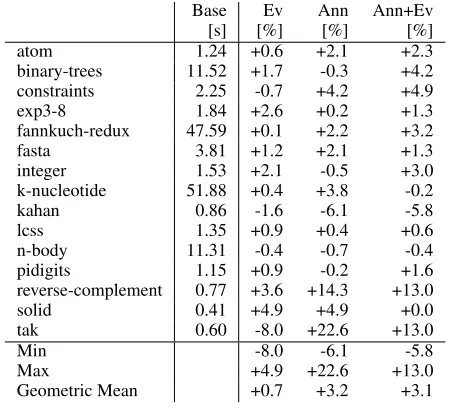
In Figure 5 we have collected benchmark results for running

thenofibbenchmark suite [15] using different configurations. We

use the GHC master development version as of 30-05-2013 as our baseline. “Ev” will mark builds with event-logging enabled, and “Ann” builds use our modified annotation-tracking compiler. All benchmarks were using the “slow” data sets on a single core of an Intel Xeon® CPU at 3.1 GHz. In order to focus on significant results and make the presentation more compact, we discarded results under 0.4 seconds run-time, and omitted them from the table if under 1 second (except notable outliers).

First consider the overhead of event-logging: Clearly the over-head is minor, showing +0.7% and -0,1% mean change respectively. The amount of spread among the benchmarks is a bit surprising though, with especially the relatively simple “tak” benchmark pro-ducing large outliers for all three configurations.

“reverse-Base Ev Ann Ann+Ev [s] [%] [%] [%]

atom 1.24 +0.6 +2.1 +2.3

binary-trees 11.52 +1.7 -0.3 +4.2 constraints 2.25 -0.7 +4.2 +4.9 exp3-8 1.84 +2.6 +0.2 +1.3 fannkuch-redux 47.59 +0.1 +2.2 +3.2 fasta 3.81 +1.2 +2.1 +1.3 integer 1.53 +2.1 -0.5 +3.0 k-nucleotide 51.88 +0.4 +3.8 -0.2 kahan 0.86 -1.6 -6.1 -5.8

lcss 1.35 +0.9 +0.4 +0.6

n-body 11.31 -0.4 -0.7 -0.4 pidigits 1.15 +0.9 -0.2 +1.6 reverse-complement 0.77 +3.6 +14.3 +13.0 solid 0.41 +4.9 +4.9 +0.0 tak 0.60 -8.0 +22.6 +13.0

Min -8.0 -6.1 -5.8

Max +4.9 +22.6 +13.0

Geometric Mean +0.7 +3.2 +3.1

Figure 5. Runtime overhead of event-logging and annotations

complement” benchmark losing about 14% of performance. Sadly, this means that our aim to be as unobtrusive to the compilation process as possible has not been completely successful, as we have to conclude that some program transformations produced different results with out annotations present. On the other hand, 3.2% mean overhead means that no important optimization has gone missing, and that the annotated program is still a valid target for profiling.

Note that we have ignored one source of overhead at this point: The cost for relocating and copying the contents of the debug sections to the event log. This often is a considerable amount of data, as it maps every single piece of machine code to both the source code as well as intermediate Core code. For example, the meta-data for profiling GHC weights around 350MB (about 5.2 million records covering 1.8 million code blocks) which take several seconds to be copied to the hard disk. However as start-up cost does not impact the validity of profiling results, we have performed all benchmarks with “stripped” executables.

6.2 Sampling Overhead

Next we consider the cost for doing actual performance measure-ments – taking samples at points of interest and writing them out to the hard disk. As mentioned before, we support three separate ways of sample collection: Hardware counter profiling, heap reten-tion profiling and heap allocareten-tion profiling. For the measurements in Figure 6, we configured all three to yield about 1000 sample val-ues per second, which is enough data to allow meaningful analysis down to time-slices of about a second.

The “Cycle” configuration uses Linux’perf_eventshardware counter kernel interface to take samples at an interval of 100,000 cycles. This method of sample collection is extremely robust, as we can delegate the actual profiling task to the operating system. From the program’s point of view, we just have to flush a memory map at regular intervals. The overhead will therefore be paid mostly in context switches to the operating system, which means that outside of timings, our program executes exactly as it would have without profiling. This means that while 8% mean overhead is not a stellar result, it is enough to support meaningful profiling.

The “Alloc” sampling method takes one sample every 4096 bytes of allocation, which we achieve through a relatively cheap run-time system change. As a result, we see that the overhead is almost not noticeable across all tests.

Ann+Ev Cycle Alloc Heap [s] [%] [%] [%]

atom 1.27 +4.4 +0.6 -0.3

binary-trees 12.01 +5.7 -0.6 +79.1 constraints 2.36 +5.4 +0.2 +15.3 exp3-8 1.87 +8.0 +0.7 +0.2 fannkuch-redux 49.13 +8.4 -0.4 +0.0 fasta 3.86 +11.5 +0.0 +0.4 integer 1.57 +9.7 -0.8 +0.0 k-nucleotide 51.78 +10.2 -0.5 -4.1

lcss 1.36 +3.5 +0.4 +4.3

n-body 11.26 +10.7 +0.0 +0.6 paraffins 0.70 +3.1 +2.0 +10.8 pidigits 1.17 +14.6 +0.0 +0.5 primes 0.69 +7.2 -2.9 -0.6 reverse-complement 0.87 +8.3 +5.1 +0.7 spectral-norm 8.26 +9.0 -0.4 +0.0

Min +3.1 -2.9 -4.1

Max +14.6 +5.1 +79.1

Geometric Mean +8.0 +0.3 +3.6

Figure 6. Runtime overhead of sampling

The “Heap” configuration on the other hand works quite differently from the first two – we are basically using GHC’s standard mech-anism for heap retention profiling [25] for our purposes. This will take snapshots of the heap at major garbage collection a minimum of 0.1 seconds apart. As a result, we can see in Figure 6 that the overhead varies a lot, depend on the heap size and the frequency of garbage collection. Note that the overhead does not reduce the quality of the memory profile, as the amount of heap retention will not change due to our analysis.

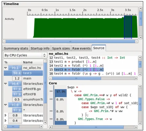
6.3 In Practice

The profiling work-flow with our tool will generally consist first of finding points in the profile that do not match expectations. It is in fact quite common to see obvious “hot spots” which provide obvious starting points. For example, we can see in Figure 4 that 98% of the time is spent in one block of Core code.

Due to optimizations, these blocks might often have quite com-plicated relations to the source code, so the second step will consist of investigating what caused the program behavior around the fo-cal point. Solutions to performance problems then often come from considering how library code and optimizations interacted with the application’s source code.

6.3.1 Example 1: String Escaping

To illustrate how this process would look like for real-life programs, let us walk through the performance analysis of some example programs. First, let us look at a program that escapes a byte-string using the blaze-builder library2:

e s c a p e : : B y t e S t r i n g → B u i l d e r e s c a p e = B .f o l d l ’ f mempty

where f b c = b ‘ mappend ‘ e s c a p e 1 c

The idea is clear: With escape1 taking care of escaping an individual character, we usefoldl’ to apply it to every byte in the string and combine results using mappend. All functions and libraries used have a great reputation for speed, so it seems reasonable to expect this approach to yield a fast program.

2_{This program was submitted to StackExchange’s code review section}

Figure 7. Profile of string escaping

However in practice we find quite the opposite: The activity time-line in Figure 7 shows that the program is actually really slow, spending just 20% of time on productive work and the rest on garbage collection! Searching for hot spots, we unsurprisingly find a specialized version of the worker of the foldl’ function busily reading bytes from the input byte-string. However, it does not seem to be writing any output right away, instead constructing lambda closures that we can identify as having blaze-builders’s “Builder” type. Using foldl’ we have merely forced the construction of a chain of builder closures instead of the result byte-string itself!

Unfortunately, this is an instance where forcing strictness does not help. We need to give blaze-builder control of the outer loop:

e s c a p e = m c o n c a t $ map e s c a p e 1 $ B . u n p a c k c

By using lists, we can now take advantage of the list fusion opti-mization [22], which eliminates intermediate closures and indeed yields a much faster loop for our example.

6.3.2 Example 2: The Glasgow Haskell Compiler

The Glasgow Haskell Compiler itself is written in Haskell, and has been under active development by Haskell experts for a long time. Therefore it simultaneously represents one of the largest and best-optimized Haskell programs available today.

This is clearly reflected in the profile (Figure 8): In contrast to previous examples, cost is spread evenly across hundreds of functions and dozens of modules. However, using our tool we can still pick out inefficiencies: For example we see a surpris-ing amount of allocation in the simplification phase between the functions “simplExprF1”, “simplIdF” and “completeCall”. Going further, we find that the code is actually allocating a number of “Outputable . SDoc” thunks, a data structure used for pretty-printing code. By selecting the thunks, we can trace them back to the defini-tion of “completeCall”, which looks roughly as follows:

c o m p l e t e C a l l : : [...] → S i m p l C o n t → SimplM [...]

c o m p l e t e C a l l [...] c o n t = do

d f l a g s ← g e t D y n F l a g s

[...]

when ( d o p t O p t _ D _ d u m p _ i n l i n i n g s d f l a g s ) $

[...] ( p p r c o n t ) [...]

Figure 8. Profile of the Glasgow Haskell Compiler

Clearly the “(ppr cont )” part only gets used in the unlikely event that we request it on the command line using-ddump-inlinings. So why does GHC allocate thunks unconditionally?

Another look into the Core code reveals that the innocent-looking call to “getDynFlags” has the effect of wrapping the whole function body into a lambda, as “SimplM” is a reader monad. This in turn makes GHC think that it would be a good idea to apply the full-laziness transformation: Float out thunks for every sub-expressions that does not depend on the “ dflags ”. This would be a very good idea if we were to call “completeCall” multiple times using different “ dflags ” every time – yet unfortunately this particular lambda will actually be evaluated exactly once.

One way to fix this is to force an earlier dependency on “ dflags ” usingseq, for example in “simplExprF1”. This indeed eliminates the allocations in question, but unfortunately does not affect pro-gram performance enough to produce measurable speed-ups.

7.

Literature

The problem of debugging and profiling optimized code has been addressed in a number of ways before, with Appel et al [2] of-fering early thoughts on how to do it in functional languages. The later works by Sansom et al [24, 25] as well as Röjemo and Runciman [23] built properly fleshed out profiling frameworks for Haskell, but still dealt with causality and optimizations in a rela-tively informal manner. Furthermore, a recent paper by Perera et al [16] tracks effects throughout a functional program in a similar manner. However, they seem to take a formal approach in deriving cause and effects, and do not consider optimizations nor applica-tions in profiling.

8.

Future Work

While we are quite confident that our profiling framework is already useful in its current state, we had to compromise on a number of issues. Firstly, while this work was inspired by the design decisions involved in building our profiler as an extension of the Glasgow Haskell Compiler, we have not formally checked that the translation fully adheres to what we can derive as the optimal annotation strategy. Especially when dealing with user rules, we probably end up with more annotations than needed.

On the technical side, we would really like to support stack tracing in some form, as it would allow us to say more about “big picture” profiling issues. Additionally, we believe that we could increase the usefulness of our profiling even more by not only tracking the effects of source code, but also of individual compiler optimizations. Cross-checking this data against both source code relations and performance data could give deeper insights into the effects of the decisions of the compiler.

9.

Conclusion

Our work aims at the heart of the supposed divide between high-level languages and high-performance programming: The notion that we cannot possibly reason about both at the same time. While optimizations indeed add complexity to the task of following causal-ity, we believe that careful analysis of compiler passes can yield an-notations that are still valid after aggressive transformations. With good profiler and user interface design, we can use these to uncover performance problems that would otherwise seem impenetrable.

Acknowledgments

We would like to thank Simon Marlow as well as the anonymous reviewers from for their helpful feedback on various versions of this paper. We would also like to thank Microsoft Research for their sponsorship through the PhD Scholarship Programme.

References

[1] DWARF debugging information format, version 2. Technical report, UNIX International Programming Languages SIG, 1993.

[2] A. W. Appel, B. F. Duba, and D. B. MacQueen. Profiling in the presence of optimization and garbage collection. Technical Report CS-TR-197-88, Princeton University, Nov 1988.

[3] G. Brooks, G. J. Hansen, and S. Simmons. A new approach to debugging optimized code. InProceedings of the SIGPLAN conference on programming language design and implementation, PLDI ’92, pages 1–11, New York, NY, USA, 1992. ACM. ISBN 0-89791-475-9. [4] D. Coutts, R. Leshchinskiy, and D. Stewart. Stream fusion: From lists to streams to nothing at all. InICFP ’07: Proceedings of the 12th ACM SIGPLAN international conference on functional programming, pages 315–326, New York, NY, USA, 2007. ACM.

[5] A. Gill and G. Hutton. The worker/wrapper transformation.Journal of Functional Programming, 19(2):227–251, Mar. 2009.

[6] A. Gill and C. Runciman. Haskell program coverage. InProceedings of the ACM SIGPLAN workshop on Haskell, Haskell ’07, pages 1–12, New York, NY, USA, 2007. ACM.

[7] A. Gill, J. Launchbury, and S. L. Peyton Jones. A short cut to defor-estation. InProceedings of the conference on functional programming languages and computer architecture, FPCA ’93, pages 223–232, New York, NY, USA, 1993. ACM.

[8] S. L. Graham, P. B. Kessler, and M. K. McKusick. gprof: A call graph execution profiler. InProceedings of the symposium on compiler construction, pages 120–126, New York, NY, USA, 1982. ACM. [9] D. Jones, Jr., S. Marlow, and S. Singh. Parallel performance tuning

for Haskell. InProceedings of the 2nd ACM SIGPLAN symposium on Haskell, Haskell ’09, pages 81–92, New York, NY, USA, 2009. ACM.

[10] S. Kaneshiro and T. Shindo. Profiling optimized code: A profiling system for an hpf compiler. InProceedings of the 10th International Parallel Processing Symposium, IPPS ’96, pages 469–473, Washing-ton, DC, USA, 1996. IEEE Computer Society.

[11] C. Lattner and V. Adve. LLVM: A compilation framework for lifelong program analysis & transformation. InProceedings of the international symposium on code generation and optimization, CGO ’04, pages 75– 86, Washington, DC, USA, March 2004. IEEE Computer Society. [12] J. Launchbury. A natural semantics for lazy evaluation. InProceedings

of the 20th ACM SIGPLAN-SIGACT symposium on principles of programming languages, POPL ’93, pages 144–154, New York, NY, USA, 1993. ACM.

[13] D. Lewis.Counterfactuals. Blackwell Publishers, Oxford, 1973. ISBN 978-0-631-22425-9.

[14] S. Marlow. Why can’t I get a stack trace? Sept. 2012. URLhaskell. org/haskellwiki/HaskellImplementorsWorkshop/2012. [15] W. Partain. Thenofibbenchmark suite of Haskell programs. In

Functional Programming, Glasgow 1992, pages 195–202. Springer, 1993.

[16] R. Perera, U. A. Acar, J. Cheney, and P. B. Levy. Functional programs that explain their work. InProceedings of the 17th ACM SIGPLAN international conference on Functional programming, ICFP ’12, pages 365–376, New York, NY, USA, 2012. ACM.

[17] S. L. Peyton Jones and A. L. M. Santos. A transformation-based optimiser for Haskell. Science of Computer Programming, 32(1-3): 3 – 47, Sep 1998. 6th European Symposium on Programming. [18] S. L. Peyton Jones and S. Marlow. Secrets of the Glasgow Haskell

compiler inliner.Journal of Functional Programming, 12(5):393–434, July 2002.

[19] S. L. Peyton Jones, C. V. Hall, K. Hammond, W. Partain, and P. Wadler. The Glasgow Haskell compiler: a technical overview. InProceedings of Joint Framework for Information Technology Technical Conference, JFIT ’93, March 1993.

[20] S. L. Peyton Jones, W. Partain, and A. Santos. Let-floating: moving bindings to give faster programs. InProceedings of the first ACM SIGPLAN international conference on functional programming, ICFP ’96, pages 1–12, New York, NY, USA, 1996. ACM.

[21] S. L. Peyton Jones, T. Nordin, and D. Oliva. C–: A portable assembly language. InImplementation of Functional Languages, pages 1–19. Springer, 1998.

[22] S. L. Peyton Jones, A. Tolmach, and T. Hoare. Playing by the rules: Rewriting as a practical optimization technique in GHC. In

Proceedings of the 2001 Haskell Workshop, Haskell ’01, pages 203– 233, Sept. 2001.

[23] N. Röjemo and C. Runciman. Lag, drag, void and use—heap profiling and space-efficient compilation revisited. InProceedings of the first ACM SIGPLAN international conference on Functional programming, ICFP ’96, pages 34–41, New York, NY, USA, 1996. ACM.

[24] P. M. Sansom. Execution Profiling for Non-strict Functional Lan-guages. PhD thesis, University of Glasgow, 1994.

[25] P. M. Sansom and S. L. Peyton Jones. Formally based profiling for higher-order functional languages. ACM Transactions on Program-ming Languages and Systems, 19(2):334–385, Mar. 1997.

[26] P. Sestoft. Deriving a lazy abstract machine. Journal of Functional Programming, 7(03):231–264, 1997.

[27] D. A. Terei and M. M. Chakravarty. An LLVM backend for GHC. In

Proceedings of the third ACM Haskell symposium, Haskell ’10, pages 109–120, New York, NY, USA, 2010. ACM.

[28] J. Tibell. State of Haskell, 2011 Survey, Aug. 2011.

URL http://blog.johantibell.com/2011/08/

results-from-state-of-haskell-2011.html.